Quantum phase transition in a multiconnected Jaynes-Cummings lattice

A MCJC lattice is composed of alternatively connected qubits and cavities. [48, 49] A schematic of a one-dimensional (1D) MCJC lattice is shown in Fig. 1, where each qubit couples to two adjacent cavities. The Hamiltonian of this model reads ($\hbar=1$)

where $\omega_{z}$ is the energy splitting of the qubits, $\omega_{c}$ is the frequency of the cavity modes, ${\sigma}_{i}^{z,+,-}$ are the Pauli matrices, ${a}_{i}$ is the annihilation operator of cavity modes, $g_{l}$ ($g_{r}$) is the coupling constant between a qubit and a cavity next to it from the left (right) hand side. In this paper, periodic boundary conditions are assumed.

Similar to the CCA model [Fig. 1(c)], a unit cell contains one qubit and one cavity. But unlike in the CCA model, the cavities are not directly coupled to each other. The unique geometry of this model renders a symmetry between $g_{l}$ and $g_{r}$, and the energy spectrum is unchanged under the exchange of these two coupling constants. This leads to the symmetry in the phase diagram discussed below.

The energy spectrum of a single unit cell in the MCJC lattice can be exactly solved. If we take a qubit with its right cavity as a unit cell [Fig. 1(a)], the Hamiltonian of the $i$th unit cell is given by

which is nothing but the standard Jaynes-Cummings (JC) model between a qubit and a cavity. [57] It has been extensively studied in cavity and circuit quantum electrodynamic (QED) systems. [58, 59, 60] In the ground state, there is no photon excitation and the qubit is in the down-spin state. If we use $|n,\sigma\rangle$ to denote the basis states, then the ground state is given by $|0,\downarrow\rangle$, where $n$ is the number of photons in the cavity and $\sigma=(\uparrow,\downarrow)$ corresponds to the two spin states of the qubit, with ground-state energy $E_{0}=-\omega_{z}/2$. The higher excitation states appear in pairs and can be regarded as a doublet, resulting from the coupling between the basis states $|n-1,\uparrow\rangle$ and $|n,\downarrow\rangle$. In this doublet subspace, the Hamiltonian can be expressed as a 2$\times 2$ matrix

There is no coupling between different doublets. Diagonalizing this matrix, we obtain the eigenstates

where $\gamma_{n+}=-\rho_{n-}=\sin\theta_{n}$, $\gamma_{n-}=\rho_{n+}=\cos\theta_{n}$, and

In the notion $|n,\pm\rangle$, $n=\langle{\sigma}_{2i-1}^{+}{\sigma}_{2i-1}^{-}+{a}_{2i}^{\dagger}{a}_{2i}\rangle$ refers to the total number of excitations in the unit cell. The corresponding eigenenergies are

where $\Delta=\omega_{z}-\omega_{c}$ is the detuning between the qubit and the cavity. At $\Delta=0$, the doublets become

and $E_{n,\pm}=(n-1/2)\omega_{c}\pm\sqrt{n}g_{r}$.

The lowest energy to excite one polariton in the JC model is $\Delta E_{1}=E_{1,-}-E_{0}$, and the energy to add the second polariton is $\Delta E_{2}=E_{2,-}-E_{1,-}$. At $\Delta=0$, $\Delta E_{1}=\omega_{c}-g_{r}$ and $\Delta E_{2}=\omega_{c}-(\sqrt{2}-1)g_{r}$. In contrast to the excitations in a bare cavity, the JC model has an intrinsic nonlinearity that can be compared to the onsite interaction in the BH model. [30] For the lower polariton states $\{|n-\rangle\}$ at $\Delta=0$, the effective on-site interaction $U\sim(2-\sqrt{2})g_{r}$, determined by the qubit-cavity coupling. Similar result can be derived at finite detuning.

In the MCJC model with finite $g_{l}$, the polariton excitations can tunnel between adjacent unit cells. The competition between the tunneling and the effective onsite repulsion strongly affects physical properties of this model. The total number of polaritons in the entire lattice

is a conserving operator. It commutes with the model Hamiltonian, $[N_{t},\,H_{t}]=0$.

We first consider the phase at an integer filling, where $N=\langle N_{t}\rangle$ is an integer multiple of the number of unit cells $L$. In the limit $g_{l}=0$, the unit cells are decoupled, and the ground state is a product state with all the unit cells being in the lower polariton states $|1,-\rangle$ and the corresponding energy is $E=NE_{1,-}$. It is in the MI phase, which has a finite energy gap for adding or removing one polariton excitation from the system.

To analyze the MCJC model at finite $g_{l}$, we adopt the polariton mapping technique [31, 40] and define a polariton operator at each unit cell

This is an operator to annihilate a $n$-polariton state at the $i$th unit cell. When $i\neq j$, $[p^{i}_{n\alpha},p^{j{\dagger}}_{m\beta}]=0$. But $p^{i}_{n\alpha}$ and $p^{i{\dagger}}_{m\beta}$ in the same unit cell do not satisfy the bosonic commutation relation. Using these operators, the spin and photon operators can be expressed as

where the coefficients are given by

and $k^{n}_{\alpha\alpha^{\prime}}=\rho_{n\alpha}\gamma_{(n-1)\alpha^{\prime}}$.

The Hamiltonian, $H_{t}$, can be represented in terms of the polariton operators. For example, at $\Delta=0$,

where

The first term in Eq. (17) describes the local polariton states with a nonlinear spectrum that resembles the effective onsite interactions. The second term in Eq. (17) can be viewed as the hopping of a polariton from site $i-1$ (reducing the number of polaritons from $m$ to $m-1$) to site $i$ (increasing the number of polaritons from $n-1$ to $n$). The competition between these two terms leads to a phase transition between the MI and SF phases. When $g_{l}=0$, the system is in the MI phase. Increasing $g_{l}$, especially in the parameter range where $g_{l}$ becomes comparable to $g_{r}$, the hopping can effectively lower the on-site interaction generated by double occupancy and drive the system into the SF phase at a critical point $g_{l}/g_{r}=\beta_{0}$. This is similar to the phase transition in the BH model with the increase of the hopping integral. [35] By further increasing $g_{l}$, another MI phase whose properties are similar to the first one by simply exchanging $g_{l}$ with $g_{r}$ emerges above a critical point $g_{l}/g_{r}=1/\beta_{0}$. This analysis agrees with the result obtained by an exact diagonalization calculation [48].

In the limit there is no coupling between different unit cells, i.e. $g_{l}=0$, at the integer filling with $N=L$, the ground state is in the MI phase with one occupation in the lower polariton state $|1,-\rangle$ per site. We denote this state as $|1111...\rangle$ and the empty site as $|0\rangle$ for simplicity. In the same limit but away from integer filling, the ground states become highly degenerate. For example, in a lattice of $L=4$ at half filling, i.e., $N=2$, the ground states are six-fold degenerate, with the following polariton configurations $|1010\rangle$, $|0101\rangle$, $|1100\rangle$, $|0110\rangle$, $|0011\rangle$, and $|1001\rangle$. In the weak intercell coupling limit, $g_{l}\ll g_{r}$, we can treat $H_{l}$ as a perturbation. In the first order approximation, the perturbed Hamiltonian can be expressed in this six-fold degenerate subspace as

By diagonalizaiton, we obtain the ground state

and the corresponding correction to the ground-state energy $E^{(1)}=-\sqrt{2}g_{l}$.

We calculate the ground-state energy, $E_{L}(N)$, of the MCJC model with $L$ unit cells and $N$ polariton excitations using the DMRG. The chemical potential for adding or removing a polariton to the ground state is then determined by the formula

$\mu_{p}$ and $\mu_{h}$ are the chemical potentials for adding and removing a polariton, respectively. [35] To obtain the chemical potentials in the thermodynamic limit, we first calculate these quantities at finite lattice systems with $L$ up to 120, and then perform an extrapolation using the formula

where $\mu_{\gamma}$ is the extrapolated chemical potential in the thermodynamic limit.

Fig. 3 shows the extrapolated chemical potentials, $\mu_{p}$ and $\mu_{h}$, as functions of $\ln(g_{l}/g_{r})$. At the integer filling with $N=L$, we find that $\mu_{p}=\mu_{h}$ in the regime $g_{l}\sim g_{r}$ (small $|\ln(g_{l}/g_{r})|$) within numerical errors. As the ratio $|\ln(g_{l}/g_{r})|$ increases, a finite difference appears between $\mu_{p}$ and $\mu_{h}$, corresponding to the opening of a finite energy gap for adding or removing a polariton. [35] Thus there is a transition from the SF phase in the small $|\ln(g_{l}/g_{r})|$ regime to the MI phase in the large $|\ln(g_{l}/g_{r})|$ regime. In the SF phase, there is no gap in the energy spectrum and $\mu_{p}=\mu_{h}$. However, in the MI phase, the energy to add or remove a polariton becomes different, and $\mu_{p}>\mu_{h}$. The extrapolated chemical potentials shown in Fig. 3 thus determine the phase boundaries that separate the MI and SF phases. If the chemical potential falls between $\mu_{p}$ and $\mu_{h}$ in the MI phase, the filling factor is fixed at $N/L=1$, and the polariton density remains a constant within this phase with zero compressibility.

At the integer filling, there are two quantum critical points which are symmetric with respect to the point $\ln(g_{l}/g_{r})=0$. The transitions between the MI and SF phases in this 1D system is of the Kosterlitz-Thouless type [62, 63]. It results from the competition between $g_{l}$ and $g_{r}$. While in the BH and CCA models, the phase transitions are due to the competition between the hopping and the onsite interaction. [32, 29, 30, 31]

The inset of Fig. 3 shows the energy gap for exciting a polariton, $E_{gp}=\mu_{p}-\mu_{h}$, as a function of $\ln(g_{l}/g_{r})$. It is clear that there is a finite regime in which $E_{gp}=0$. But we cannot accurately determine the positions of the critical points, where $E_{gp}$ begins to deviate from zero, just from the result of this energy gap.

At half filling, the results of chemical potentials indicate that there is no difference in the energy for adding or removing a polariton, i.e. $\mu_{p}=\mu_{h}$, in the whole parameter regime. Thus there is no MI-SF phase transition and the ground state is always in the SF phase.

The single-particle density matrices for the qubits and cavities are defined respectively by,

They measure the correlations of polariton excitations. [64, 65]

Fig. 4 shows the normalized single-particle density matrices $\Gamma_{r}(i-j)/\Gamma_{r}(0)$ and $\Gamma_{q}(i-j)/\Gamma_{q}(0)$ versus $i-j$ for two sets of parameters. At the integer filling, $N/L=1$, both density matrices drop exponentially to zero with the increase of the distance between the two unit cells in the MI phase, $g_{l}/g_{r}\ll 1$. In the SF phase, however, the two density matrices remain finite even in the large distance limit, indicating the existence of superfluid off-diagonal long-range order. At half filling, $N/L=1/2$, the ground state is in the SF phase, and the two density matrices behave qualitatively similar to the case of $g_{l}=g_{r}$ at the integer filling: they decrease with the increase of the distance between the two unit cells and saturate to certain finite values in the large distance limit.

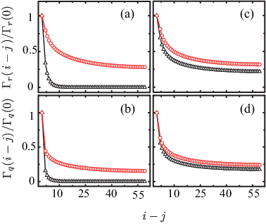
The single-particle density matrices can be fitted using the formulae

where $\xi_{q}$ ($\xi_{r}$) is the correlation length between two qubits (cavities). Fig. 5(a) shows the coefficients $y_{q}$ and $y_{r}$ as functions of $\ln(g_{l}/g_{r})$. As expected, both $y_{q}$ and $y_{r}$ are zero in the MI phase, but become finite in the SF phase around the regime $\ln(g_{l}/g_{r})$ close to 0.

The correlation lengths, shown in Fig. 5(b), increase quickly around the critical points in the MI phases. But we do not see the divergence of the correlation lengths at the critical point, due to the finite lattice size effect. At the critical point, the entanglement entropy is expected to grow logarithmically with the system size. Thus in order to accurately determine the critical points from the divergent correlation lengths, we need to enlarge not just the lattice size, but also the number of states retained in the DMRG calculation.

From the density-density correlation functions, we calculate the structure factors of the qubits and cavities, defined by

where ${n}_{i}^{r}={a}_{i}^{{\dagger}}{a}_{i}$ and ${n}_{i}^{q}={\sigma}_{i}^{+}{\sigma}_{i}^{-}$. Fig. 6 shows $S_{\pi}^{q}$ and $S_{\pi}^{r}$ as functions of $1/L$ at half filling and $g_{l}=0.0055$, $g_{r}=0.0245$. Within numerical errors, the extrapolated structure factors are found to be approximately zero, indicating that there is no crystalline or CDW ordered phases in this system at half filling. [34]

In the 1D SF phase, the ground state is a Luttinger liquid, [62, 63] and the correlation functions should decay algebraically with the distance between the unit cells

where $K_{\alpha}$ is the Luttinger parameter. Our calculation, as shown in Fig. 7, has indeed confirmed this power law dependence for the single-particle density matrices. The deviation from the power-law dependence at large distance results from the finite-size effect. The power-law behaviors have also been observed at half filling, where the ground state is always in the SF phase. In contrast, in the MI phase, the single-particle density matrices decay exponentially with the distance.

$K_{q}$ and $K_{r}$ are important parameters for characterizing the critical behavior of the MCJC model. To obtain the Luttinger parameters in the thermodynamic limit, an extrapolation of the finite lattice results to the $L\rightarrow\infty$ limit is needed. From the numerical results, we find that $K_{\alpha}$ ($\alpha=q,r$) can be well fitted by the formula (see the insets of Fig. 7)

where $K^{0}_{\alpha}$ is the extrapolated Luttinger parameter in the limit $L\rightarrow\infty$ and $\lambda_{\alpha}$ is a coefficient.

The MI-SF phase transition at integer fillings is of the Kosterlitz-Thouless type, and $K_{q}^{0}=K_{r}^{0}=1/2$ are expected at the critical points for $N/L=1$. [34, 62, 63] In contrast, the corresponding commensurate-uncommensurate phase transitions satisfy $K_{q}^{0}=K_{r}^{0}=1$. From the calculation of these Luttinger parameters, we can accurately determine the critical points. Fig. 8 shows $K_{q}^{0}$ and $K_{r}^{0}$ as functions of $\ln(g_{l}/g_{r})$ for the MCJC model at the integer filling $N/L=1$. Within numerical accuracy, we find that $K_{q}^{0}=K_{r}^{0}$ in the whole parameter range we have studied. Deep in the SF phase, $g_{l}\sim g_{r}$, $K_{q,r}^{0}<1/2$, indicating that the spatial correlation decreases slowly with the distance. As $|\ln(g_{l}/g_{r})|$ is increased, $K_{q,r}^{0}$ increase and cross the points $K^{0}_{q,r}=1/2$ at $\beta_{0}=g_{l}/g_{r}\approx 0.579$ and $1/\beta_{0}=g_{l}/g_{r}\approx 1.727$. The Luttinger parameters at half filling, as shown in the inset of Fig. 8, are found to be $1/2<K_{\alpha}^{0}<2$, indicating no phase transition in the whole parameter regime studied.