Hierarchical Symbolic Dynamic Filtering of Streaming Non–stationary Time Series Data

Dynamical systems generate time series data which lie in the space of continuous or discrete signals. In the symbolic dynamic filtering literature [25], quantization of the continuous (in this case streaming–type) signals (or in some cases already discrete signals) into symbol sequences is a major first step in the $SDF$ formulation. There are many ways of quantization (or partitioning as called in the Symbolic Dynamics literature) reported in the literature [30, 31, 32] depending on different objective functions. However, the focus of this paper is to model symbol sequences (using $PFSA$ models) obtained after such quantization.

Given a suitably defined nonempty, finite set of symbols called alphabet $\Xi$, and nonempty, finite set of states $\Theta$, we define a $PFSA$, $\mathcal{P}$ as a 4–tuple, such that $\mathcal{P}\triangleq(\Theta,\Xi,\delta,\Omega)$. Nonlinearities in the time series are represented by a specific type of $PFSA$ called the D–Markov machines [33] where past depth D of symbols are considered for modeling the states as given by $|\Theta|\leq|\Xi|^{D}$ [25]. The mapping $\delta:\Theta\times\Xi\rightarrow\Theta$ denotes a function that maps the transitions from a current state to a future state (or self transition) given the alphabet. Also, we consider a morph function $\pi:\Theta\times\Xi\rightarrow[0,1]$ that satisfies the condition $\sum_{\xi\in\Xi}\pi(\theta,\xi)=1$. Based on the morph function, we define the non-negative $(|\Theta|\times|\Xi|)$ state transition matrix $\Omega$ as: $\Omega_{ij}\triangleq\pi(\theta_{i},\xi_{j}),\forall\theta_{i}\in\Theta$ and $\forall\xi_{j}\in\Xi$. Online learning of an $SDF$ model involves identifying this matrix.

Note that initial state $\theta_{0}\in\Theta$ of the quasi–stationary data represented by the $\mathcal{P}\triangleq(\Theta,\Xi,\delta,\Omega)$ have no influence on the state transition. However, a simple frequency count of the occurrence of symbols in the training string sequence at depth $D$, followed by normalization is used to derive the low dimensional encoding matrix $\Omega$. With that knowledge, new testing symbol strings that also follow the same quantization can be evaluated for similarity or difference with a $PFSA$ represented by $\Omega$.

This subsection briefly describes a couple of basic statistical concepts used in the proposed formulation, namely the Chinese Restaurant Process ($CRP$) and data likelihood adjustment using the stickiness factor. Recently, these ideas have been extensively used in nonparametric modeling techniques and therefore details can be found in the related literature [34, 10].

$CRP$ represents a discrete sequence over partitions that is suitable for modeling infinite mixtures, hence often used for modeling clusters in Bayesian frameworks. $CRP$ shares some similarities with the stick breaking and the Dirichlet Process, but with some subtle differences in how the processes evolve [34]. The crux of the $CRP$ distribution is to model the tendencies of newly arriving customers to a fictional Chinese restaurant to either sit in an existing table $\in O$ or in a new table, $o_{new}$ [35] with less restriction on number of tables or customers at a table (as illustrated in Figure 2). Therefore, $CRP$ is a suitable candidate for nonparametric modeling. The CRP distribution can be mathematically described as follows:

where $\mathbb{C}(\cdot)$ signifies a concentration function and $\epsilon$ is called the $CRP$ parameter. Naturally, this paper uses a $CRP$ process to determine whether a new $PFSA$ model is required to model a newly arriving slow time epoch or an existing PFSA would suffice.

While induction of $CRP$ can help in deciding the need for a new $PFSA$ model, noise and spurious disturbance present in real data can drive the decision system to instability. That is, many unnecessary new $PFSA$ models may get generated and the decision may then fluctuate among different $PFSA$ models that are close to each other, with closeness based on an appropriate metric. Similar situation arises in other unsupervised techniques as well such as the HDP–HMM. Assuming inference could be made after the arrival of several slow time epochs, an off–line revision that is described in Subsection3.3 will be effective at merging such spurious classes. However, in most real–life application, decisions have to be taken in an online manner, i.e., soon after the arrival of the new slow time epochs. A stickiness factor described by [10, 26] was found to be effective for reducing such fluctuations. The extra information incorporated by stickiness is to lean slightly towards the class occupied by the most recently assigned (before the current epoch) slow time epoch. The ideas discussed in this section are described mathematically in Section 3.

Let us assume that $K$ classes representing $K$ unique quasi–stationary behavior occurred in the past data epochs have already been identified. Let the distinct set of classes be $\{C^{i}:i=1,2,\cdots,K\}$, over the same sets of symbol $\Xi$ and state $\Theta$, and each class $C^{i}$ is modeled by a PFSA $\mathcal{P}^{i}=(\Theta^{i},\Xi,\delta^{i},\Omega^{i})$. Also, let symbol strings belonging to the class be $S^{i}\triangleq s^{i}_{1}s^{i}_{2}\ldots$. An appropriate depth $D$ is selected for the $D$–Markov machine from which the morph (probability) matrix $\Omega^{i}$ has been derived. Each row of the $\Omega$ is normalized in order to perform inference on a new slow time epoch.
Let the $m^{th}$ row of $\Omega^{i}$ be denoted as $\Omega^{i}_{m}$ and the $n^{th}$ element of the $m^{th}$ row as $\Omega^{i}_{mn}\geq 0$ and $\sum_{n=1}^{|\Xi|}\Omega^{i}_{mn}=1$. The a priori probability density function $f_{\Omega^{i}_{m}|S^{i}}$ of the random row-vector $\Omega^{i}_{m}$ that is conditioned on a symbol string $S^{i}$ can be modeled by the Dirichlet distribution [36, 37] as,

where, each column of the $\Omega^{i}$ is represented by $\boldsymbol{\omega}^{i}_{m}$ as,

and the constant for normalization is

where, $\Gamma(\bullet)$ denotes the gamma function, and $\boldsymbol{\alpha}^{i}_{m}=\begin{bmatrix}\boldsymbol{\alpha}^{i}_{m1}&\boldsymbol{\alpha}^{i}_{m2}&\ldots&\boldsymbol{\alpha}^{i}_{m|\Xi|}\end{bmatrix}$ with

At a state $\theta_{m}$, the number of times the symbol $\xi_{n}$ arises in the transition to a new state is modeled by $N^{i}_{mn}$ as,

where $s_{k}^{i}$ is the $k^{th}$ symbol in $S^{i}$ and $v_{k}^{i}$ is the $k^{th}$ state as obtained from the symbol sequence $S^{i}$. Note that a state is defined as a sequence of past D symbols. $N^{i}_{m}\triangleq\sum_{n=1}^{|\Xi|}N^{i}_{mn}$ computes the number that state $\theta_{m}$ occur in the state sequence. From Equation 4 and Equation 5, it follows that

where the standard definition, $\Gamma(n)=(n-1)!\ \ \forall n\in\mathbb{N}$ has been used.
Markov property of the $PFSA\ \mathcal{P}^{i}$, ensures that the $(1\times|\Xi|)$–dimension row vectors of $\Omega^{i}$ are statistically independent of each other, $\forall m=1,\ldots|\Theta|$. Equation 4 and Equation 7 thus lead to conditioning of the a priori joint density, $f_{\Omega^{i}|S^{i}}$ of the probability morph matrix, $\Omega^{i}$ on the symbol string, $S^{i}$ as,

where, $\boldsymbol{\omega}^{i}=\Big[(\boldsymbol{\omega}_{1}^{i})^{T}\ (\boldsymbol{\omega}_{2}^{i})^{T}\ \cdots\ (\boldsymbol{\omega}_{|\Theta|}^{i})^{T}\Big]\in[0,1]^{|\Theta|\times|\Xi|}$, and $T$ is a transpose operator.
At this point, if a new slow time test epoch is represented by $\widetilde{S}$, its probability of belonging to a certain $PFSA$ model $(\Theta,\Xi,\delta,\Omega^{i})$, given the morph matrix $\Omega^{i}$ derived from the training symbol sequence $S^{i}$ can be represented as a product of multinomial distributions [38] as,

where, given a state $\theta_{m}$, the number of times the symbol $\xi_{n}$ present in the testing string $\widetilde{S}$ occurs during transition to a new state is modeled by $\widetilde{N}_{mn}$ as,

where again, the $k^{th}$ symbol in the observed string $\widetilde{S}$ is $\tilde{s}_{k}$, and the $k^{th}$ state derived from $\widetilde{S}$ is denoted by $\tilde{v}_{k}$.
Now, Equation 8 and Equation 9 can be combined to obtain the probability of a symbol string $\widetilde{S}$ belonging to a class characterized by already observed symbol string $S^{j}$. With the derivation presented by [39], the following conditional distribution was obtained,

where $\widetilde{N}_{m}\triangleq\sum_{n=1}^{|\Xi|}\widetilde{N}_{mn}$. In practice, Stirling’s approximation for the logarithm of a factorial $\log(n!)\approx n\log(n)-n$ [40] is mostly easier to compute, especially when either (or both) of $N^{i}$ and $\widetilde{N}$ consist of statistically large enough sample points (but still not be enough to directly estimate a $\Pi$ matrix at the testing phase). At this point, the likelihood probability, $\Pr(\widetilde{S}|S^{i})$ may be easily found by normalizing the conditional factors in Equation 12.

The objective of the inference process is to compute the probability of assigning a slow time epoch $\tau_{j}$ to a class $C^{i}\in\textbf{C}$ (where $\textbf{C}=\{C^{i}\ \forall\ i=1,\cdots,K\}$ is the set of existing classes) or a newly created class $C^{K+1}$. Let the symbol sequence for the current slow time epoch be $\widetilde{S}_{\tau_{j}}$. Then the likelihood for class $C^{i}$ for current epoch $\tau_{j}$ is given by $\mu(\widetilde{S}_{\tau_{j}}|S^{i})$ as described in the previous subsection. The posterior probability for class selection can be denoted by $\Pr(C^{i},S^{i}|\widetilde{S}_{\tau_{j}})$ which is equivalent to $\Pr(C^{i}|\widetilde{S}_{\tau_{j}})$ in this case since all existing classes are completely characterized by symbol sequences $S^{i}\ \forall i$. With this setup, we obtain the following:

We use the Chinese Restaurant Process ($CRP$) to introduce the likelihood of a new class $C^{K+1}$ with a $CRP$ hyperparameter $\gamma_{j}$ as follows (note that the hyperparameter is specific to the test epoch $\tau_{j}$).

$CRP$ hyperparameter $\gamma_{j}$ (that was described in Equation 2) is given by the following expression.

where, $\epsilon\geq 0$ is a real valued parameter and $\mu(\widetilde{S}_{\tau_{j}}|S^{i})$ is treated as the concentration or strength function found in Equation 1 and Equation 2 for the $CRP$ formulation. However, instead of the classical formulation [26], we introduce a new scalar multiplier b that modifies the likelihood of creating a new class. The choice of b will depend on a parameter $\textbf{A}(\Delta,i)$ that captures the rate of change of data likelihood as follows:

where $\Delta$ is a memory parameter that accommodates likelihoods of past epochs. It is evident from the expression of $\textbf{A}(\Delta,i)$ that it is essentially an expected reduction of likelihood of exisiting classes at the current epoch $\tau_{j}$. A high value of $\Delta$ reduces the noise in estimation, which can also reduce the senstivity to class changes. While $\textbf{A}(\Delta,i)$ can be incorporated in various ways to compute the $CRP$ parameter, it is accommodated in a discrete manner in the present formulation. Note that the condition with high values of $\textbf{A}(\Delta,i)\ \forall i$ suggests a significant drop in likelihood of all existing classes which increases the possibility of a new class generation. Therefore, a positive threshold, $\nu$ is chosen such that when $\textbf{A}(\Delta,i)>\nu\ \forall i$, we use $\textbf{b}=1$ (i.e., classical formulation). Otherwise, we reduce the possibility of new class generation by taking $\textbf{b}=2$ for the adaptive $CRP$ formulation.
At this point, we introduce the notion of ‘stickiness’ in our proposed algorithm which is based on the fact that a real–life system usually may not fluctuate its operating point or internal parametric condition at each slow time epoch. In the present context, this means that if a slow time epoch $\tau_{j-1}$ belongs to a class, $C^{k}\in\textbf{C}$, then there will be a high likelihood for new streaming data at epoch $\tau_{j}$ to belong to $C^{k}$ as well. This notion is incorporated into the formulation by introducing a positive bias towards the last seen class $C^{k}$ as follows:

where $0<\kappa<1$ is the stickiness factor. Note, the rationale behind this adjustment is to ensure a certain minimum likelihood for the last seen class $C^{k}$ and in this context, the proposed formulation ensures that

This can be proved by considering the extreme case when $\mu_{\gamma}(C^{k}|\widetilde{S}_{\tau_{j}})=0$, before applying the stickiness factor. Numerically, the ‘stickiness’ adjustment significantly reduces the ‘hunting behavior’ in class identification and creation process which will be demonstrated via numerical simulation results in the next section.
Finally, the $\mu_{\gamma_{j}}(C^{i}|\widetilde{S}_{\tau_{j}})$ factors are normalized to obtain the posterior probabilities $\Pr(C^{i}|\widetilde{S}_{\tau_{j}})$ for each class as follows:

We generate a random sample from this distribution to take a decision of class identification and generation at the testing epoch $\tau_{j}$.
The online algorithm for class assignment is summarized below. Note, we assume that partitioning and state construction are already performed before we begin the following algorithm. Hence, the alphabet $\Xi$ and state set $\Theta$ and the corresponding indices $n$ and $m$ are already defined.

Algorithm 1 operates at the lowest logical layer in an online manner for learning multiple PFSA models representing different unique quasi–stationary characteristics. Representation of these characteristics is performed by considering the changes in the data likelihood and its rate of change. However, when the data quality is low especially in term of signal-to-noise ratio (SNR), the online learning algorithm may generate many spurious classes. In such cases, redundant PFSA models may be pruned periodically, that is, after a few slow time epochs have been observed. The pruning step proposed here merges different $PFSA$ models whose proximity are evaluated with the metric laid out in the Definition 3.1 below (according to [33]).

Thus, the pruning step can merge two different $PFSA$ models identified by online $HSDF$, $\mathcal{P}^{1}$ and $\mathcal{P}^{2}$ when $\Phi(\mathcal{P}^{1},\mathcal{P}^{2})<\eta$, where $\eta>0$. In this paper, the metrics have been evaluated on symbols whose word length are $1$. Note that this revision step can be considered to be part of an off–line process for learning the higher-level (Tier 2) PFSA.

The gamma function $\Gamma(\alpha)$ can be expressed as,

Using Stirling’s approximation, the expression can be simplified under the assumption of $\alpha\gg\frac{1}{2}$ as the following:

Using this formula, we can rewrite the normalizing constant described in our online classification approach (see Equation 4) as

By eliminating common terms from the numerator and the denominator, we obtain

Let the constant denominator term $(\sum_{n=1}^{|\Xi|}\alpha^{i}_{mn})^{(\sum_{n=1}^{|\Xi|}\alpha^{i}_{mn})}$ be denoted as $Z=(N^{i}_{m}+|\Xi|)^{N^{i}_{m}+|\Xi|}$. With this setup Equation 8 can be rewritten as

Similarly, at the testing stage, Equation 10 can be rewritten as

where $\widetilde{Z}=(\widetilde{N}_{m})^{\widetilde{N}_{m}}$.

Proof Sketch:

After some algebraic rearrangement we obtain,

Note that $\sum_{m=1}^{|\Theta|}\log(\widetilde{Z})$ is a constant normalization factor term and $\Omega_{mn}^{i}$ represents the models learnt at the training stage for the existing classes (hence, does not change significantly). Therefore, if we aim to maximize the log-likelihood $\log\Pr\left(\widetilde{S}|\Omega^{i}\right)$ over all models (or classes) denoted by the index $i$, we obtain

where $\widetilde{\alpha}$ represents the distribution of the testing data and $\Omega^{i}$ represents the training data distribution (for model $i$).

We use the chaotic Duffing system described by Equation 30 which is a popular choice as a nonlinear system [29].

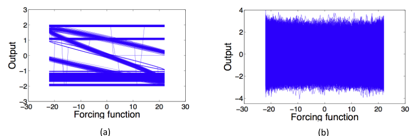
where $A=22.0$ is the input amplitude, w = 5.0 rad/s is its frequency of excitation, excitation harmonics, $\alpha_{1}$ = 1.0, stiffness, $\lambda$ = 1.0. It is know that varying $\beta$, the dissipation parameter causes change in the system behavior and a sudden shift or bifurcation occurs around $\beta=0.3$ [14]. Hence, $\beta=0.1$ signifies an operating region before bifurcation and $\beta=0.4$ represents a system behavior after bifurcation. Therefore, a non-stationary time series with two types of quasi-stationary segments can be generated by randomly selecting between the two $\beta$ values for different segments. Plots of the output $x$ vs. the forcing function are shown in Figure 3 under different noise contamination levels.

We also extended the system to generate data with three types of quasi-stationary segments or features by adding a Van der Pol oscillation system behavior which is given by [44]

Figure 4 shows the plots of the output $x$ vs. the forcing function with all the three features (two from the Duffing system and one from the Van der Pol system) under two different noise contamination levels. For both 2–features and 3–features cases, time series data with randomly generated $400$ epochs (with $1000$ data points of one particular feature in each epoch) are used for testing. Also for symbolic dynamic analysis, the raw time series is symbolized with a uniform partitioning (i.e., equal width binning) into $7$ bins that is found to be sufficient experimentally for most cases.

We evaluate the performance of the proposed algorithm on both the two and three features test cases. However, we begin with analysis to explore the effects of adaptive $CRP$ formulation with parameter b, stickiness adjustment and off–line revision steps.

Performance with classical $CRP$ formulation: Many traditional methods only consider data likelihood for feature change detection or outlier detection purposes. However, in our proposed algorithm, we also utilize the change in data likelihood to decide on generating new models. We incorporate the effect of change in likelihood via using the adaptive $CRP$ formulation with parameter b. While in our algorithm, b can take a value of $1$ or $2$ depending on the parameter $\textbf{A}(\Delta,i)$ ($\Delta$ is chosen to be $4$ for the results in this paper), the classical $CRP$ formulation would use a constant $\textbf{b}=1$. Figure 5 presents the results using the classical formulation, where plate (a) shows the performance only after applying the $CRP$ step, plate (b) shows the effect of stickiness adjustment and plate (c) provides the final result after the off-line revision step (using $\eta=\frac{1}{2K}$ given $K$ classes from the online part, i.e., after stickiness adjustment). While the $CRP$ step enables the framework to detect changes in time series characteristics, evidently, the stickiness adjustment is critical to control the ‘hunting’ behavior and create ‘too many’ new classes. Finally, the off–line $PFSA$ revision step helps to improve the result even further. Note, this result is obtained using a noiseless (i.e., signal to noise ratio, $SNR=\infty$) data set with two features. Figure 6 presents the effect of noise content (for $SNR=\infty$, $SNR=9$ and $SNR=1$) on the performance using the same algorithm (i.e., constant $\textbf{b}=1$). The results demonstrate visually that the algorithm is quite robust to significant noise contamination.

Performance with adaptive $CRP$ formulation: Now we move to the adaptive $CRP$ formulation as described in Algorithm 1, with an appropriate choice of b (i.e., equal to 1 or 2) based on the change in data likelihood of the existing classes. Results are presented in Figure 7 that show the adaptive formulation (with stickiness adjustment) to be quite efficient and achieves online performance better than that obtained after off–line revision with the classical formulation. Similar to the previous case, the algorithm is also quite stable under noise contamination.

Additionally, we found that the sensitivity of the algorithm to the hyper-parameters, $\epsilon$ and $\kappa$ reduces significantly under the adaptive $CRP$ formulation. Typically, the values for $\epsilon$ and $\kappa$ used in this paper are $\approx 0.02$ and $\approx 0.6$ respectively. Figure 8 shows the data log-likelihood plots for the class transitions and new class creation in an explicit manner. Table 1 compiles all the quantitative results for both classical and adaptive $CRP$ formulation under the different noise conditions considered here. The results show that online $HSDF$ with adaptive $CRP$ performs the best under low to moderate noise level. At a higher noise level, the off–line revision may be more suitable.

Performance comparison: We compared the results from our proposed algorithm with those from Hierarchical Dirichlet Process – Hidden Markov Model (HDP–HMM) [10] that is a sampling based technique based on the Bayesian nonparametric concept, such that the joint distribution of the states are derived from the Dirichlet process. HDP–HMM techniques have been used in learning switching linear dynamical systems ($SLDS$). Note that the idea of stickiness has been adopted from the HDP--HMM literature as we aim to extract features for more realistic and general cases of nonlinear dynamical systems in a fast and computationally efficient manner. For comparison purposes, we implemented the codes made available on the authors’ webpage ¹¹ 1 https://www.stat.washington.edu/ ebfox/software.html that uses a Gaussian observed model type with Normal–Inverse–Wishart ($NIW$) prior, which we found to be producing best results for all use cases. The results for the HDP–HMM approach under the noiseless ($SNR=\infty$) and the most noisy ($SNR=1$) cases are shown in Figure 9. Note that the HDP–HMM [10] algorithm classifies each data point individually, being a sampling technique. Hence, a majority voting was done to select the most prominent class in each epoch (i.e., $1000$ data points as defined earlier) for a more realistic comparison. From the plots, it is quite evident visually that our proposed approach has better accuracy which can be explained by the fact that $SDF$ inherently is an efficient way to model nonlinear system behavior.

Also, the performance of the HDP-HMM approach suffers significantly in the presence of a large amount of noise in the signal. However, we note that HDP–HMM approach correctly identifies the number of features present in the non–stationary time series data which is significant. We performed further comparison using the 3–features case, and present the results in Figure 10 and Figure 11 for the $SNR=\infty$ and $SNR=1$ cases respectively. It can be observed that our algorithm still performs better in both the identification of the total number of features present in the time series data as well as in classifying them. Finally, the quantitative performance of $HSDF$ and HDP–HMM (Gaussian $NIW$) for the two and three features cases are summarized in Table 2. Note, the smaller time requirement for our proposed algorithm compared to that of HDP–HMM is primarily due to the fact that there is no sampling step or latent variable involved in the HSDF approach. The computation time reported here is achieved with MATLAB implementations on a $2.1$ GHz Intel Xeon(R), $1200$ MHz CPU with $64$GB RAM and UNIX OS.

References

- [1] D. Bruckner, R. Velik, Y. Penya, Machine perception in automation: A call to arms, EURASIP Journal on Embedded Systems 2011 (608423) (2011) 1–9.
- [2] G. Hinton, R. Salakhutdinov, Reducing the dimensionality of data with neural networks, Science 313.5786 (2006) 504–507.
- [3] Y. Bengio, O. Delalleau, Algorithmic Learning Theory, Vol. 6925, Springer Berlin Heidelberg, 2011, Ch. On the expressive power of deep architectures, pp. 18–36.
- [4] K. G. Lore, A. Akintayo, S. Sarkar, Llnet: A deep autoencoder approach to natural low-light image enhancement, Elsevier Journal of Pattern Recognition 61 (2017) 650–662.
- [5] A. Akintayo, K. G. Lore, S. Sarkar, S. Sarkar, Prognostics of combustion instabilities from hi-speed flame video using a deep convolutional selective autoencoder, International Journal of Prognostics and Health Management (special issue) 7 (023) (2016) 1–14.
- [6] A. Akintayo, N. Lee, V. Chawla, M. Mullaney, C. Marett, A. Singh, A. Singh, G. Tylka, B. Ganapathysubramanian, S. Sarkar, An end-to-end convolutional selective autoencoder approach to soybean cyst nematode eggs detection, Knowledge Discovery and Data Mining workshop on Data Science for Food, Energy and Water (2016) 1–8.
- [7] K. G. Lore, D. Stoecklein, M. Davies, B. Ganapathysubramanian, S. Sarkar, Hierarchical feature extraction for efficient design of microfluidic flow patterns, Proceeedings of the 1st International workshop on "Feature Extraction: Modern Questions and Challenges", NIPS (2015) 213–225.
- [8] Z. C. Lipton, J. Berkowitz, C. Elkan, A critical review of recurrent neural networks for sequence learning, arXiv:1506.00019v4 (2015) 1–38.
- [9] F. A. Gere, J. Schmidhuber, F. Cummins, Learning to forget: Continual prediction with lstm, IEEE Journal on Neural Computation 12 (10) (2000) 2451–2471.
- [10] E. B. Fox, E. B. Sudderth, M. I. Jordan, A. S. Willsky, A sticky hdp-hmm with application to speaker diarization, The Annals of Applied Statistics 5 (2A) (2011) 1020–1056.
- [11] S. Tranter, D. Reynolds, An overview of automatic speaker diarisation systems, IEEE Transactions on Speech, Audio and Language Processing: Special Issue on Rich Transcription (2006) 1557–1565.
- [12] J. B. Tenenbaum, C. Kemp, T. L. Griffiths, N. D. Goodman, How to grow a mind: Statistics, structure, and abstraction, Science 331 (2011) 1279–1285.
- [13] S. Sarkar, S. Sarkar, K. Mukherjee, A. Ray, A. Srivastav, Multi-sensor data interpretation and semantic fusion for fault detection in aircraft gas turbine engines, Proceedings of the I Mech E Part G: Journal of Aerospace Engineering 227 (12) (December 2013) 1988–2001.
- [14] C. Rao, A. Ray, S. Sarkar, M. Yasar, Review and comparative evaluation of symbolic dynamic filtering for detection of anomaly patterns, Signal, Image, and Video Processing 3 (2009) 101–114.
- [15] X. Jin, Y. Guo, S. Sarkar, A. Ray, R. M. Edwards, Anomaly detection in nuclear power plants via symbolic dynamic filtering, IEEE Transactions on Nuclear Science 58 (1) (2011) 277–288.
- [16] S. Chakraborty, S. Sarkar, S. Gupta, A. Ray, Damage monitoring of refractory wall in a generic entrained-bed slagging gasification system, Proceedings of the I Mech E Part A: Journal of Power and Energy 222, Part A (8) (October 2008) 791–807.
- [17] S. Sarkar, N. Virani, M. Yasar, A. Ray, S. Sarkar, Spatiotemporal information fusion for fault detection in shipboard auxiliary systems, American Control Conference, Washington D. C. (987-1-4799-0178-4) (2013) 3846–3851.
- [18] S. Sarkar, M. Yasar, S. Gupta, A. Ray, K. Mukherjee, Fault detection and isolation in aircraft gas turbine engines: Part ii - validation on a simulation test bed, Proceedings of the I Mech E Part G: Journal of Aerospace Engineering 222 (3) (May 2008) 319–330.
- [19] S. Gupta, A. Ray, S. Sarkar, M. Yasar, Fault detection and isolation in aircraft gas turbine engines: Part i - underlying concept, Proceedings of the I Mech E Part G: Journal of Aerospace Engineering 222 (3) (May 2008) 307–318.
- [20] C. Liu, S. Ghosal, Z. Jiang, S. Sarkar, An unsupervised spatiotemporal graphical modeling approach to anomaly detection in cps, Proceedings of the International Conference on Cyber-physical Systems (ICCPS) (2016) 1 – 10.
- [21] Z. Jiang, S. Sarkar, Understanding wind turbine interactions using spatiotemporal pattern network, Proceedings of the ASME 2015 Dynamic Systems and Control Conference (2015) 1–10.
- [22]
C. Liu, Y. Gong, S. Laflamme, B. Phares, S. Sarkar,
Bridge damage
detection using spatiotemporal patterns extracted from dense sensor network,
Measurement Science and Technology 28 (1) (2017) 014011.
URL http://stacks.iop.org/0957-0233/28/i=1/a=014011 - [23] S. Sarkar, Z. Jiang, A. Akintayo, S. Krishnamurthy, A. Tewari, Probabilistic graphical modeling of distributed cyber-physical systems, in: H. Song, D. Rawat, S. Jeschke, C. Brecher (Eds.), Cyber-Physical Systems: Foundations, Principles and Applications, 1st Edition, no. 9780128038017, Todd Green, 2016, Ch. 18, pp. 265–286.
- [24] S. Sarkar, S. Sarkar, A. Ray, Data-enabled Health Management of Complex Industrial Systems, Fault Detection: Classification, Techniques and Role in Industrial Systems, NOVA Science Publishers, 2014.
- [25] A. Ray, Symbolic dynamic analysis of complex systems for anomaly detection, Elsevier Journal of Signal Processing 84 (7) (2004) 1115–1130.
- [26] A. Akintayo, S. Sarkar, A symbolic dynamic filtering approach to unsupervised hierarchical feature extraction from time-series data, American Control Conference (2015) 5824–5829.
- [27] S. Sarkar, T. Damarla, A. Ray, Real-time activity recognition from seismic signature via multi-scale symbolic time series analysis (mstsa), American Control Conference (10.1109) (2015) 5818–5823.
- [28] E. B. Fox, E. B. Sudderth, M. I. Jordan, A. S. Willsky, Nonparametric bayesian learning of switching linear dynamical systems, Advances in Neural Information Processing Systems (2009) 457–464.
- [29] C. Rao, K. Mukherjee, S. Sarkar, A. Ray, Statistical estimation of multiple parameters via symbolic dynamic filtering, Signal Processing 89 (2009) 981 – 988.
- [30] S. Sarkar, A. Srivastav, A composite discretization scheme for symbolic identification of complex systems, Signal Processing 125 (2016) 156 – 170.
- [31] S. Sarkar, A. Srivastav, M. Shashanka, Maximally bijective discretization for data-driven model of complex systems, American Control Conference, Washington D. C. (978-1-4799-0178-4) (2013) 2674–2679.
- [32] S. Sarkar, K. Mukherjee, X. Jin, A. Ray, Optimization of symbolic feature extraction from time-series for classification, Signal Processing 92 (3) (March 2012) 625–635.
- [33] K. Mukherjee, A. Ray, State splitting and merging in probabilistic finite state automata for signal representation and analysis, Signal processing 104 (2014) 105 –119.
- [34] Y. W. Teh. A tutorial on dirichlet processes and hierarchical dirichlet processes [online] (March 2007).
- [35] D. J. Aldous, Exchangeability and related topics in Lecture Notes in Mathematics, Vol. 1117, Springer Berlin Heidelberg, 1985.
- [36] T. S. Ferguson, A bayesian analysis of some nonparametric problems, The Annals of Statistics 1 (2) (1973) 209–230.
- [37] J. Sethuraman, A constructive definition of dirichlet priors, Statistica Sinica 4 (1994) 639–650.
- [38] S. Wilks, Mathematical Statistics, John Wiley, New York, NY, USA, 1963.
- [39] S. Sarkar, K. Mukherjee, S. Sarkar, A. Ray, Symbolic dynamic analysis of transient time series for fault detection in gas turbine engines, Technical Brief DS-11-1309, The Pennsylvania State University, University Park, PA 16802, to appear in J. Dyn. Sys. Meas. Control (2000).
- [40] R. Pathria, Statistical Mechanics, 2nd Edition, Butterworth-Heinemann, Oxford, UK, 1996.
- [41] S. Kullback, R. Liebler, On information and sufficieny, The annals of mathematical statistics (1951) 79–86.
- [42] N. L. Roux, Y. Bengio, Representational power of restricted boltzmann machines and deep belief networks, Neural Computation 20.6 (2008) 1631–1649.
- [43] Y. Bengio, Learning deep architectures for ai, Foundations and Trends in Machine Learning (2009) 1–71.
- [44] M. Tsatsos, Theoretical and numerical study of the van der pol equation, Ph.D. thesis, Aristotle University of Thessaloniki, School of Sciences (July 2006).