跳到论文正文
W Papers独立论文阅读器 arXiv:1702.01491 论文正文 计算阅读时间 · 0%
引用这篇论文根据当前论文元数据生成,正式投稿前建议核对。


License: arXiv.org perpetual non-exclusive license
arXiv:1702.01491v2 [math.NA] 26 Jun 2017

Adaptive Quasi-Monte Carlo Methods for Cubature

Fred J. Hickernell    Lluís Antoni Jiménez Rugama    Da Li Affiliation: Fred J. Hickernell (✉), Lluís Antoni Jiménez Rugama Affiliation: Illinois Institute of Technology, RE 208, 10 W. 32nd{}^{\text{nd}} St., Chicago, USA
E-mail: hickernell@iit.edu; ljimene1@hawk.iit.edu; dli37@hawk.iit.edu
Abstract

High dimensional integrals can be approximated well by quasi-Monte Carlo methods. However, determining the number of function values needed to obtain the desired accuracy is difficult without some upper bound on an appropriate semi-norm of the integrand. This challenge has motivated our recent development of theoretically justified, adaptive cubatures based on digital sequences and lattice nodeset sequences. Our adaptive cubatures are based on error bounds that depend on the discrete Fourier transforms of the integrands. These cubatures are guaranteed for integrands belonging to cones of functions whose true Fourier coefficients decay steadily, a notion that is made mathematically precise. Here we describe these new cubature rules and extend them in two directions. First, we generalize the error criterion to allow both absolute and relative error tolerances. We also demonstrate how to estimate a function of several integrals to a given tolerance. This situation arises in the computation of Sobol’ indices. Second, we describe how to use control variates in adaptive quasi-Monte cubature while appropriately estimating the control variate coefficient.

1 Introduction

An important problem studied by Ian Sloan is evaluating multivariate integrals by quasi-Monte Carlo methods. After perhaps a change of variable, one may pose the problem as constructing an accurate approximation to

μ=∫[0,1)df(𝒙)d𝒙,\mu=\int_{[0,1)^{d}}f({\bm{x}})\,\mathrm{d}{\bm{x}},

given a black-box function ff that provides f⁡(𝒙)f({\bm{x}}) for any 𝒙∈[0,1)d{\bm{x}}\in[0,1)^{d}. Multivariate integrals arise in applications such as evaluating financial risk, computing multivariate probabilities, statistical physics, and uncertainty quantification.

We have developed and implemented quasi-Monte Carlo (qMC) cubature algorithms that adaptively determine the sample size needed to guarantee that an error tolerance is met provided that the integrand belongs to a cone 𝒞{\mathcal{C}} of well-behaved functions [2, 11, 13, 15]. That is, given a low discrepancy sequence 𝒙0,𝒙1,…{\bm{x}}_{0},{\bm{x}}_{1},\ldots and function data f⁡(𝒙0),f⁡(𝒙1),…f({\bm{x}}_{0}),f({\bm{x}}_{1}),\ldots, we have a stopping rule based on the function data obtained so far that chooses nn for which

|μ−μ^n|≤ε,where ​μ^n=1n​∑i=0n−1f⁡(𝒙i),f∈𝒞.\left\lvert\mu-\widehat{\mu}_{n}\right\rvert\leq\varepsilon,\qquad\text{where }\widehat{\mu}_{n}=\frac{1}{n}\sum_{i=0}^{n-1}f({\bm{x}}_{i}),\quad f\in\mathcal{C}. (1)

Here, μ^n\widehat{\mu}_{n} is the sample average of function values taken at well-chosen points whose empirical distribution mimics the uniform distribution. The cone 𝒞{\mathcal{C}} contains integrands whose Fourier coefficients decay in a reasonable manner, thus allowing the stopping rule to succeed. Specifically, the size of the high wavenumber components of an integrand in 𝒞{\mathcal{C}} cannot be large in comparison to the size of the low wavenumber components. Rather than choosing the 𝒙i{\bm{x}}_{i} to be independent and identically distributed (IID) 𝒰[0,1)d\mathcal{U}[0,1)^{d} points, we use shifted digital sequences [4, 19] and sequences of nodesets of shifted rank-11 lattices [10, 17, 18, 23]. Sequences that are more evenly distributed than IID points are the hallmark of qMC algorithms.

Traditional qMC error analysis leads to error bounds of the form [3, 8]

|μ−μ^n|≤D⁡({𝒙i}i=0n−1)​∥f∥,\left\lvert\mu-\widehat{\mu}_{n}\right\rvert\leq D(\{{\bm{x}}_{i}\}_{i=0}^{n-1})\lVert f\rVert,

where the integrand, ff, is assumed to lie in some Banach space with (semi-)norm ∥⋅∥\lVert\cdot\rVert, and ∥f∥\lVert f\rVert is often called the variation of ff. Moreover, the discrepancy D⁡(⋅)D(\cdot) is a measure of quality of the sample, {𝒙i}i=0n−1\{{\bm{x}}_{i}\}_{i=0}^{n-1}. For integrands lying in the ball ℬ:={f:∥f∥≤σ}{\mathcal{B}}:=\{f:\lVert f\rVert\leq\sigma\} one may construct a non-adaptive algorithm guaranteeing |μ−μ^n|≤ε\left\lvert\mu-\widehat{\mu}_{n}\right\rvert\leq\varepsilon by choosing n=min⁡{n′∈ℕ:D⁡({𝒙i}i=0n′−1)≤ε/σ}n=\min\bigl\{n^{\prime}\in{\mathbb{N}}:D(\{{\bm{x}}_{i}\}_{i=0}^{n^{\prime}-1})\leq\varepsilon/\sigma\bigr\}.

Our interest is in adaptive qMC algorithms, where nn depends on the the function data observed. Several heuristics have been proposed for choosing nn:

Independent and identically distributed (IID) replications. [21]

Compute

μ^n,R=1R∑r=1Rμ^n(r),μ^n(r)=1n∑i=0n−1f(𝒙i(r)),r=1,…,R,\widehat{\mu}_{n,R}=\frac{1}{R}\sum_{r=1}^{R}\widehat{\mu}^{(r)}_{n},\qquad\widehat{\mu}_{n}^{(r)}=\frac{1}{n}\sum_{i=0}^{n-1}f({\bm{x}}_{i}^{(r)}),\quad r=1,\ldots,R,

where {𝒙i(1)}i=0∞,…,{𝒙i(R)}i=0∞\bigl\{{\bm{x}}_{i}^{(1)}\bigr\}_{i=0}^{\infty},\ldots,\bigl\{{\bm{x}}_{i}^{(R)}\bigr\}_{i=0}^{\infty} are IID randomizations of a low discrepancy sequence, and 𝔼⁡(μ^n(r))=μ{\mathbb{E}}\bigl(\widehat{\mu}^{(r)}_{n}\bigr)=\mu. The standard deviation of these μ^n(r)\widehat{\mu}^{(r)}_{n}, perhaps multiplied by an inflation vector is proposed as an upper bound for |μ−μ^n,R|\lvert\mu-\widehat{\mu}_{n,R}\rvert.

Internal replications. [21]

Compute

μ^n​R=1R∑r=1Rμ^n(r)=1n​R∑r=1n​Rf(𝒙i),μ^n(r)=1n∑i=(r−1)​nr​n−1f(𝒙i),r=1,…,R.\widehat{\mu}_{nR}=\frac{1}{R}\sum_{r=1}^{R}\widehat{\mu}^{(r)}_{n}=\frac{1}{nR}\sum_{r=1}^{nR}f({\bm{x}}_{i}),\qquad\widehat{\mu}_{n}^{(r)}=\frac{1}{n}\sum_{i=(r-1)n}^{rn-1}f({\bm{x}}_{i}),\quad r=1,\ldots,R.

The standard deviation of these μ^n(r)\widehat{\mu}^{(r)}_{n}, perhaps multiplied by an inflation vector is proposed as an upper bound for |μ−μ^n​R|\lvert\mu-\widehat{\mu}_{nR}\rvert.

Quasi-standard error. [7]

Compute

μ^n,R=1R∑r=1Rμ^n(r),μ^n(r)=1n∑i=0n−1f(𝒙i,(r−1)​d+1:r​d),r=1,…,R,\widehat{\mu}_{n,R}=\frac{1}{R}\sum_{r=1}^{R}\widehat{\mu}^{(r)}_{n},\qquad\widehat{\mu}_{n}^{(r)}=\frac{1}{n}\sum_{i=0}^{n-1}f({\bm{x}}_{i,(r-1)d+1:rd}),\quad r=1,\ldots,R,

where {𝒙i}i=0∞\{{\bm{x}}_{i}\}_{i=0}^{\infty} is now an R​dRd dimensional sequence, and 𝒙i,(r−1)​d+1:r​d{\bm{x}}_{i,(r-1)d+1:rd} denotes the (r−1)​d+1st(r-1)d+1^{\text{st}} through r​dthrd^{\text{th}} components of the ithi^{\text{th}} point in the sequence. The standard deviation of these μ^n(r)\widehat{\mu}^{(r)}_{n}, perhaps multiplied by an inflation vector is proposed as an upper bound for |μ−μ^n,R|\lvert\mu-\widehat{\mu}_{n,R}\rvert. However, see [22] for cautions regarding this method.

None of the above methods have theoretical justification. Since the proposed error bounds are homogeneous, it is clear that the sets of integrands for which these error bounds are correct are cones. That is, if one of the above error bounds above is correct for integrand ff, it is also correct for integrand c​fcf, where cc is an arbitrary constant. Unfortunately, there is no theorem defining a cone 𝒞{\mathcal{C}} for which any of the above error bounds must succeed.

In this article we review our recent work developing adaptive qMC algorithms satisfying (1). We describe the cones 𝒞{\mathcal{C}} for which our algorithms succeed. We also extend our earlier algorithms in two directions:

  • •

    Meeting more general error criteria than simply absolute error, and

  • •

    Using control variates to improve efficiency.

Our data-based cubature error bounds are described in Sec. 2. This section also emphasizes the similar algebraic structures of our two families of qMC sequences. In Sec. 3, we describe how our error bounds can be used to satisfy error criteria that are more general than that in (1). Sec. 4 describes the implementation of our new adaptive qMC algorithms and provides numerical examples. Control variates with adaptive qMC cubature is described in Sec. 5. We conclude with a discussion that identifies problems for further research.

2 Error Estimation for Digital Net and Lattice Cubature

Here we summarize some of the key properties of cubature based on digital sequences and rank-11 lattice node sequences. We use a common notation for both cases to highlight the similarities in analysis. We focus on the base 22 setting for simplicity and because it is most common in practice. Moreover, n=2mn=2^{m} for non-negative integer mm. See [11] and [15] for more details.

Let {𝟎=𝒛0,𝒛1,…}\{{\bm{0}}={\bm{z}}_{0},{\bm{z}}_{1},\ldots\} be a sequence of distinct points that is either a digital sequence or a rank-11 lattice node sequence. Let ⊕:[0,1)d×[0,1)d→[0,1)d\oplus:[0,1)^{d}\times[0,1)^{d}\to[0,1)^{d} denote an addition operator under which the sequence is a group and the first 2m2^{m} points form a subgroup. For some shift, 𝚫∈[0,1)d{\bm{\Delta}}\in[0,1)^{d}, the data sites used for cubature in (1) are given by 𝒙i=𝒛i⊕𝚫{\bm{x}}_{i}={\bm{z}}_{i}\oplus{\bm{\Delta}} for all i∈ℕ0i\in{\mathbb{N}}_{0}. Typical examples of a digital sequence and a rank-11 lattice node sequence are given in Fig. 1.

Refer to caption
Refer to caption
Figure 1: Two dimensional projections of a digitally shifted and Owen scrambled digital sequence (left) and a shifted rank-1 lattice node set (right).

There is a set of integer vector wavenumbers, 𝕂{\mathbb{K}}, which is a group under its own addition operator, also denoted ⊕\oplus. There is also a a bilinear functional, ⟨⋅,⋅⟩:𝕂×[0,1)d→ℝ\langle\cdot,\cdot\rangle:{\mathbb{K}}\times[0,1)^{d}\to{\mathbb{R}}, which is used to to define a Fourier basis for L2[0,1)dL^{2}[0,1)^{d}, given by {e2​π​−1​⟨𝒌,⋅⟩}𝒌∈𝕂\bigl\{\mathrm{e}^{2\pi\sqrt{-1}\langle{\bm{k}},\cdot\rangle}\bigr\}_{{\bm{k}}\in{\mathbb{K}}}. The integrand is expressed as a Fourier series,

f(𝒙)=∑𝒌∈𝕂f^(𝒌)e2​π​−1​⟨𝒌,𝒙⟩∀𝒙∈[0,1)d,f∈L2[0,1)d,where f^(𝒌):=∫[0,1)df(𝒙)e−2​π​−1​⟨𝒌,𝒙⟩d𝒙.f({\bm{x}})=\sum_{{\bm{k}}\in{\mathbb{K}}}\hat{f}({\bm{k}})\mathrm{e}^{2\pi\sqrt{-1}\langle{\bm{k}},{\bm{x}}\rangle}\quad\forall{\bm{x}}\in[0,1)^{d},\ f\in L^{2}[0,1)^{d},\\ \text{where }\hat{f}({\bm{k}}):=\int_{[0,1)^{d}}f({\bm{x}})\mathrm{e}^{-2\pi\sqrt{-1}\langle{\bm{k}},{\bm{x}}\rangle}\,\mathrm{d}{\bm{x}}. (2)

Since we require function values for cubature, we assume throughout that this Fourier series is absolutely convergent, i.e., ∑𝒌∈𝕂|f^​(𝒌)|<∞\sum_{{\bm{k}}\in{\mathbb{K}}}\lvert\hat{f}({\bm{k}})\rvert<\infty.

In the case of digital sequences, ⊕\oplus denotes digit-wise addition modulo 22 for points in [0,1)d[0,1)^{d} and wavenumbers in 𝕂=ℕ0d{\mathbb{K}}={\mathbb{N}}_{0}^{d}. The digits of 𝒛1,𝒛2,𝒛4,𝒛8,…{\bm{z}}_{1},{\bm{z}}_{2},{\bm{z}}_{4},{\bm{z}}_{8},\ldots correspond to elements in the generator matrices for the usual method for constructing digital sequences (4, Sec. 4.4). Also, ⟨𝒌,𝒙⟩\langle{\bm{k}},{\bm{x}}\rangle is one half of an ℓ2\ell^{2} inner product of the digits of 𝒌{\bm{k}} and 𝒙{\bm{x}} modulo 22. The e2​π​−1​⟨𝒌,⋅⟩\mathrm{e}^{2\pi\sqrt{-1}\langle{\bm{k}},\cdot\rangle} are multivariate Walsh functions (see Fig. 2).

Refer to caption Refer to caption Refer to caption
Figure 2: One-dimensional Walsh functions corresponding to k=0,1,2,3,4k=0,1,2,3,4, and 55.

In the case of rank-1 lattice node sequences, ⊕\oplus denotes addition modulo 𝟏{\bm{1}} for points in [0,1)d[0,1)^{d} and ordinary addition for wavenumbers in 𝕂=ℤd{\mathbb{K}}={\mathbb{Z}}^{d}. Moreover, ⟨𝒌,𝒙⟩=𝒌T​𝒙mod1\langle{\bm{k}},{\bm{x}}\rangle={\bm{k}}^{T}{\bm{x}}\bmod 1. The e2​π​−1​⟨𝒌,⋅⟩\mathrm{e}^{2\pi\sqrt{-1}\langle{\bm{k}},\cdot\rangle} are multivariate complex exponential functions.

The dual set corresponding to the first n=2mn=2^{m} unshifted points, {𝒛0,…,𝒛2m−1}\{{\bm{z}}_{0},\ldots,{\bm{z}}_{2^{m}-1}\}, is denoted 𝕂m{\mathbb{K}}_{m} and defined as

𝕂0:=𝕂,𝕂m:={𝒌∈𝕂:⟨𝒌,𝒛2ℓ⟩=0 for all ℓ=0,…,m−1},m∈ℕ.{\mathbb{K}}_{0}:={\mathbb{K}},\qquad{\mathbb{K}}_{m}:=\{{\bm{k}}\in{\mathbb{K}}:\langle{\bm{k}},{\bm{z}}_{2^{\ell}}\rangle=0\text{ for all }\ell=0,\ldots,m-1\},\quad m\in{\mathbb{N}}.

The dual set satisfies

12m​∑i=02m−1e2​π​−1​⟨𝒌,𝒛i⟩={1,𝒌∈𝕂m,0,otherwise.\frac{1}{2^{m}}\sum_{i=0}^{2^{m}-1}\mathrm{e}^{2\pi\sqrt{-1}\langle{\bm{k}},{\bm{z}}_{i}\rangle}=\begin{cases}1,&{\bm{k}}\in{\mathbb{K}}_{m},\\ 0,&\text{otherwise}.\end{cases}

The discrete Fourier transform of a function ff using n=2mn=2^{m} data is denoted f~m\tilde{f}_{m} and defined as

f~m​(𝒌)\displaystyle\tilde{f}_{m}({\bm{k}}) :=12m​∑i=02m−1f⁡(𝒙i)​e−2​π​−1​⟨𝒌,𝒙i⟩\displaystyle:=\frac{1}{2^{m}}\sum_{i=0}^{2^{m}-1}f({\bm{x}}_{i})\mathrm{e}^{-2\pi\sqrt{-1}\langle{\bm{k}},{\bm{x}}_{i}\rangle}
=f^​(𝒌)+∑𝒍∈𝕂m∖{𝟎}f^​(𝒌⊕𝒍)​e2​π​−1​⟨𝒍,𝚫⟩,\displaystyle=\hat{f}({\bm{k}})+\sum_{{\bm{l}}\in{\mathbb{K}}_{m}\setminus\{{\bm{0}}\}}\hat{f}({\bm{k}}\oplus{\bm{l}})\mathrm{e}^{2\pi\sqrt{-1}\langle{\bm{l}},{\bm{\Delta}}\rangle}, (3)

after applying some of the properties alluded to above. This last expression illustrates how the discrete Fourier coefficient f~m​(𝒌)\tilde{f}_{m}({\bm{k}}) differs from its true counterpart, f^​(𝒌)\hat{f}({\bm{k}}), by the aliasing terms, which involve the other wavenumbers in the coset 𝒌⊕𝕂m{\bm{k}}\oplus{\mathbb{K}}_{m}. As mm increases, wavenumbers leave 𝕂m{\mathbb{K}}_{m}, and so the aliasing decreases.

The sample mean of the function data is the 𝒌=𝟎{\bm{k}}={\bm{0}} discrete Fourier coefficient:

μ^n=12m​∑i=02m−1f⁡(𝒙i)=f~m​(𝟎)=∑𝒍∈𝕂mf^​(𝒍)​e2​π​−1​⟨𝒍,𝚫⟩.\widehat{\mu}_{n}=\frac{1}{2^{m}}\sum_{i=0}^{2^{m}-1}f({\bm{x}}_{i})=\tilde{f}_{m}({\bm{0}})=\sum_{{\bm{l}}\in{\mathbb{K}}_{m}}\hat{f}({\bm{l}})\mathrm{e}^{2\pi\sqrt{-1}\langle{\bm{l}},{\bm{\Delta}}\rangle}.

Hence, an error bound for the sample mean may be expressed in terms of those Fourier coefficients corresponding to wavenumbers in the dual set:

|μ−μ^n|=|f^​(𝟎)−f~m​(𝟎)|=|∑𝒍∈𝕂m∖{𝟎}f^​(𝒍)​e2​π​−1​⟨𝒍,𝚫⟩|≤∑𝒍∈𝕂m∖{𝟎}|f^​(𝒍)|.\left\lvert\mu-\widehat{\mu}_{n}\right\rvert=\left\lvert\hat{f}({\bm{0}})-\tilde{f}_{m}({\bm{0}})\right\rvert=\left\lvert\sum_{{\bm{l}}\in{\mathbb{K}}_{m}\setminus\{{\bm{0}}\}}\hat{f}({\bm{l}})\mathrm{e}^{2\pi\sqrt{-1}\langle{\bm{l}},{\bm{\Delta}}\rangle}\right\rvert\leq\sum_{{\bm{l}}\in{\mathbb{K}}_{m}\setminus\{{\bm{0}}\}}\left\lvert\hat{f}({\bm{l}})\right\rvert. (4)

Our aim is to bound the right hand side of this cubature error bound in terms of function data or more specifically, in terms of the discrete Fourier transform. However, this requires that the true Fourier coefficients of the integrand do not decay too erratically. This motivates our definition of 𝒞{\mathcal{C}}, the cone of integrands for which our adaptive algorithms succeed.

To facilitate the definition of 𝒞{\mathcal{C}} we construct an ordering of the wavenumbers, 𝒌~:ℕ0→𝕂\tilde{{\bm{k}}}:{\mathbb{N}}_{0}\to\mathbb{K} satisfying 𝒌~​(0)=𝟎\tilde{{\bm{k}}}(0)={\bm{0}} and {𝒌~​(κ+λ​2m)}λ=0∞=𝒌~​(κ)⊕𝕂m\bigl\{\tilde{{\bm{k}}}(\kappa+\lambda 2^{m})\bigr\}_{\lambda=0}^{\infty}=\tilde{{\bm{k}}}(\kappa)\oplus{\mathbb{K}}_{m} for κ=0,…,2m−1\kappa=0,\ldots,2^{m}-1 and m∈ℕ0m\in{\mathbb{N}}_{0}, as described in [11, 15]. This condition implies the crucial fact that |f~m​(𝒌~​(κ+λ​2m))|\left\lvert\tilde{f}_{m}(\tilde{{\bm{k}}}(\kappa+\lambda 2^{m}))\right\rvert is the same for all λ∈ℕ0\lambda\in{\mathbb{N}}_{0}. Although there is some arbitrariness in this ordering, it is understood that 𝒌~​(κ)\tilde{{\bm{k}}}(\kappa) generally increases in magnitude as κ\kappa tends to infinity. We adopt the shorthand notation f^κ:=f^​(𝒌~​(κ))\hat{f}_{\kappa}:=\hat{f}(\tilde{{\bm{k}}}(\kappa)) and f~m,κ:=f~m​(𝒌~​(κ))\tilde{f}_{m,\kappa}:=\tilde{f}_{m}(\tilde{{\bm{k}}}(\kappa)). Then, the error bound in (4) may be written as

|μ−μ^n|≤∑λ=1∞|f^λ​2m|.\left\lvert\mu-\widehat{\mu}_{n}\right\rvert\leq\sum_{\lambda=1}^{\infty}\left\lvert\hat{f}_{\lambda 2^{m}}\right\rvert. (5)

The cone of functions whose Fourier series are absolutely convergent and whose true Fourier coefficients, f^κ\hat{f}_{\kappa}, decay steadily as κ\kappa tends to infinity is

𝒞={f∈AC([0,1)d):S^ℓ,m(f)≤ω^(m−ℓ) S
 

      ⋀     


m(f),ℓ≤m,
 S
 

      ⋀     


m(f)≤ω̊(m−ℓ)Sℓ(f),ℓ∗≤ℓ≤m},
\mathcal{C}=\{f\in AC([0,1)^{d}):\widehat{S}_{\ell,m}(f)\leq\widehat{\omega}(m-\ell)\hbox{\hskip 8.33334pt\hskip-3.35416pt\hbox{$S$}\hskip-3.35416pt\hskip-8.33334pt\raisebox{17.83344pt}{\hbox{$\scalebox{-1}{\hbox{\lx@scalerel@obj{\lx@scalerel@obj{\lx@scalerel@obj{\kern-0.6pt\bigwedge\kern-0.6pt}}}}}$}}\hskip-8.33334pt\hskip 8.33334pt}_{m}(f),\ \ \ell\leq m,\\ \hbox{\hskip 8.33334pt\hskip-3.35416pt\hbox{$S$}\hskip-3.35416pt\hskip-8.33334pt\raisebox{17.83344pt}{\hbox{$\scalebox{-1}{\hbox{\lx@scalerel@obj{\lx@scalerel@obj{\lx@scalerel@obj{\kern-0.6pt\bigwedge\kern-0.6pt}}}}}$}}\hskip-8.33334pt\hskip 8.33334pt}_{m}(f)\leq\mathring{\omega}(m-\ell)S_{\ell}(f),\ \ \ell_{*}\leq\ell\leq m\},
(6a)
where
Sm​(f):=∑κ=⌊2m−1⌋2m−1|f^κ|,S^ℓ,m​(f):=∑κ=⌊2ℓ−1⌋2ℓ−1∑λ=1∞|f^κ+λ​2m|,\displaystyle S_{m}(f):=\sum_{\kappa=\left\lfloor 2^{m-1}\right\rfloor}^{2^{m}-1}\left\lvert\hat{f}_{\kappa}\right\rvert,\qquad\widehat{S}_{\ell,m}(f):=\sum_{\kappa=\left\lfloor 2^{\ell-1}\right\rfloor}^{2^{\ell}-1}\sum_{\lambda=1}^{\infty}\left\lvert\hat{f}_{\kappa+\lambda 2^{m}}\right\rvert, (6b)
 S
 

      ⋀     


m
​(f)
:=S^0,m​(f)+⋯+S^m,m​(f)=∑κ=2m∞|f^κ|
,
\displaystyle\hbox{\hskip 8.33334pt\hskip-3.35416pt\hbox{$S$}\hskip-3.35416pt\hskip-8.33334pt\raisebox{17.83344pt}{\hbox{$\scalebox{-1}{\hbox{\lx@scalerel@obj{\lx@scalerel@obj{\lx@scalerel@obj{\kern-0.6pt\bigwedge\kern-0.6pt}}}}}$}}\hskip-8.33334pt\hskip 8.33334pt}_{m}(f):=\widehat{S}_{0,m}(f)+\cdots+\widehat{S}_{m,m}(f)=\sum_{\kappa=2^{m}}^{\infty}\left\lvert\hat{f}_{\kappa}\right\rvert,
(6c)

and where ℓ,m∈ℕ0\ell,m\in{\mathbb{N}}_{0} and ℓ≤m\ell\leq m. The positive integer ℓ∗\ell_{*} and the bounded functions ω^,ω̊:ℕ0→[0,∞)\widehat{\omega},\mathring{\omega}:{\mathbb{N}}_{0}\to[0,\infty) are parameters that determine how inclusive 𝒞{\mathcal{C}} is and how robust our algorithm is. Moreover, ω̊​(m)→0\mathring{\omega}(m)\to 0 as m→∞m\to\infty. The default values are provided in Sec. 4.

We now explain the definition of the cone 𝒞{\mathcal{C}} and the data driven cubature error bound that we are able to derive. For illustration we use the functions depicted in Fig. 3. The one on the left lies inside 𝒞{\mathcal{C}} because its Fourier coefficients decay steadily (but not necessarily monotonically), while the one on the right lies outside 𝒞{\mathcal{C}} because its Fourier coefficients decay erratically. The function lying outside 𝒞{\mathcal{C}} resembles the one lying inside 𝒞{\mathcal{C}} but with high wavenumber noise.

The sum of the absolute value of the Fourier coefficients appearing on the right side of error bound (5) is S^0,m​(f)\widehat{S}_{0,m}(f) according to the definition in (6b). In Fig. 3, m=11m=11, and S^0,11​(f)\widehat{S}_{0,11}(f) corresponds to the sum of |f^κ|\lvert\hat{f}_{\kappa}\rvert for κ=2​048,4​096,6​144,…\kappa=2~048,4~096,6~144,\ldots. Since only n=2mn=2^{m} function values are available, it is impossible to estimate the Fourier coefficients appearing in S^0,m​(f)\widehat{S}_{0,m}(f) directly by discrete Fourier coefficients.

By the definition in (6c), it follows that S^0,m​(f)≤ S
 

      ⋀     


m
​(f)
\widehat{S}_{0,m}(f)\leq\hbox{\hskip 8.33334pt\hskip-3.35416pt\hbox{$S$}\hskip-3.35416pt\hskip-8.33334pt\raisebox{17.83344pt}{\hbox{$\scalebox{-1}{\hbox{\lx@scalerel@obj{\lx@scalerel@obj{\lx@scalerel@obj{\kern-0.6pt\bigwedge\kern-0.6pt}}}}}$}}\hskip-8.33334pt\hskip 8.33334pt}_{m}(f)
. In Fig. 3,  S
 

      ⋀     


11
​(f)
\hbox{\hskip 8.33334pt\hskip-3.35416pt\hbox{$S$}\hskip-3.35416pt\hskip-8.33334pt\raisebox{17.83344pt}{\hbox{$\scalebox{-1}{\hbox{\lx@scalerel@obj{\lx@scalerel@obj{\lx@scalerel@obj{\kern-0.6pt\bigwedge\kern-0.6pt}}}}}$}}\hskip-8.33334pt\hskip 8.33334pt}_{11}(f)
corresponds to the sum of all |f^κ|\lvert\hat{f}_{\kappa}\rvert with κ≥2048\kappa\geq 2048. The definition of 𝒞{\mathcal{C}} assumes that S^0,m​(f)≤ω^​(m)​ S
 

      ⋀     


m
​(f)
\widehat{S}_{0,m}(f)\leq\widehat{\omega}(m)\hbox{\hskip 8.33334pt\hskip-3.35416pt\hbox{$S$}\hskip-3.35416pt\hskip-8.33334pt\raisebox{17.83344pt}{\hbox{$\scalebox{-1}{\hbox{\lx@scalerel@obj{\lx@scalerel@obj{\lx@scalerel@obj{\kern-0.6pt\bigwedge\kern-0.6pt}}}}}$}}\hskip-8.33334pt\hskip 8.33334pt}_{m}(f)
, where ω^​(m)\widehat{\omega}(m) could be chosen as 11 or could decay with mm. This is up to the user.

Refer to caption Refer to caption
Figure 3: A typical function lying inside 𝒞{\mathcal{C}} and its Fourier Walsh coefficients (left) in contrast to a function lying outside 𝒞{\mathcal{C}} and its Fourier Walsh coefficients (right).

Still,  S
 

      ⋀     


m
​(f)
\hbox{\hskip 8.33334pt\hskip-3.35416pt\hbox{$S$}\hskip-3.35416pt\hskip-8.33334pt\raisebox{17.83344pt}{\hbox{$\scalebox{-1}{\hbox{\lx@scalerel@obj{\lx@scalerel@obj{\lx@scalerel@obj{\kern-0.6pt\bigwedge\kern-0.6pt}}}}}$}}\hskip-8.33334pt\hskip 8.33334pt}_{m}(f)
involves Fourier coefficients that are of too high a wavenumber to be approximated by discrete Fourier coefficients. The definition of 𝒞{\mathcal{C}} also assumes that  S
 

      ⋀     


m
​(f)
≤ω̊​(r)​Sm−r​(f)
\hbox{\hskip 8.33334pt\hskip-3.35416pt\hbox{$S$}\hskip-3.35416pt\hskip-8.33334pt\raisebox{17.83344pt}{\hbox{$\scalebox{-1}{\hbox{\lx@scalerel@obj{\lx@scalerel@obj{\lx@scalerel@obj{\kern-0.6pt\bigwedge\kern-0.6pt}}}}}$}}\hskip-8.33334pt\hskip 8.33334pt}_{m}(f)\leq\mathring{\omega}(r)S_{m-r}(f)
for any non-negative r≤m−ℓ∗r\leq m-\ell_{*}. This means that the infinite sum of the high wavenumber coefficients,  S
 

      ⋀     


m
​(f)
\hbox{\hskip 8.33334pt\hskip-3.35416pt\hbox{$S$}\hskip-3.35416pt\hskip-8.33334pt\raisebox{17.83344pt}{\hbox{$\scalebox{-1}{\hbox{\lx@scalerel@obj{\lx@scalerel@obj{\lx@scalerel@obj{\kern-0.6pt\bigwedge\kern-0.6pt}}}}}$}}\hskip-8.33334pt\hskip 8.33334pt}_{m}(f)
cannot exceed some factor, ω̊​(r)\mathring{\omega}(r), of the finite sum of modest wavenumber coefficients Sm−r​(f)S_{m-r}(f). In Fig. 3, r=4r=4, and the graph on the left shows  S
 

      ⋀     


11
​(f)
\hbox{\hskip 8.33334pt\hskip-3.35416pt\hbox{$S$}\hskip-3.35416pt\hskip-8.33334pt\raisebox{17.83344pt}{\hbox{$\scalebox{-1}{\hbox{\lx@scalerel@obj{\lx@scalerel@obj{\lx@scalerel@obj{\kern-0.6pt\bigwedge\kern-0.6pt}}}}}$}}\hskip-8.33334pt\hskip 8.33334pt}_{11}(f)
to be bounded above by ω̊​(4)​S7​(f)\mathring{\omega}(4)S_{7}(f) for a modest value of ω̊​(4)\mathring{\omega}(4). Recall from the definition in (6b) that S7​(f)S_{7}(f) is the sum of the absolute value of the Fourier coefficients corresponding to 64,…,12764,\ldots,127. However, the function depicted in the right of Fig. 3 violates the assumption that  S
 

      ⋀     


11
​(f)
≤ω̊​(4)​S7​(f)
\hbox{\hskip 8.33334pt\hskip-3.35416pt\hbox{$S$}\hskip-3.35416pt\hskip-8.33334pt\raisebox{17.83344pt}{\hbox{$\scalebox{-1}{\hbox{\lx@scalerel@obj{\lx@scalerel@obj{\lx@scalerel@obj{\kern-0.6pt\bigwedge\kern-0.6pt}}}}}$}}\hskip-8.33334pt\hskip 8.33334pt}_{11}(f)\leq\mathring{\omega}(4)S_{7}(f)
because S7​(f)S_{7}(f) in that case is very small. Thus, the function on the right in Fig. 3 lies outside 𝒞{\mathcal{C}}.

Based on the above argument, it follows in general that for f∈𝒞f\in{\mathcal{C}},

∑λ=1∞|f^λ​2m|=S^0,m​(f)≤ω^​(m)​ S
 

      ⋀     


m
​(f)
≤ω^​(m)​ω̊​(r)​Sm−r​(f)
,
m≥r+ℓ∗≥ℓ∗.
\sum_{\lambda=1}^{\infty}\left\lvert\hat{f}_{\lambda 2^{m}}\right\rvert=\widehat{S}_{0,m}(f)\leq\widehat{\omega}(m)\hbox{\hskip 8.33334pt\hskip-3.35416pt\hbox{$S$}\hskip-3.35416pt\hskip-8.33334pt\raisebox{17.83344pt}{\hbox{$\scalebox{-1}{\hbox{\lx@scalerel@obj{\lx@scalerel@obj{\lx@scalerel@obj{\kern-0.6pt\bigwedge\kern-0.6pt}}}}}$}}\hskip-8.33334pt\hskip 8.33334pt}_{m}(f)\leq\widehat{\omega}(m)\mathring{\omega}(r)S_{m-r}(f),\\ m\geq r+\ell_{*}\geq\ell_{*}.
(7)

This implies an error bound in terms of the true Fourier coefficients with modest wavenumber. In particular (7) holds for the function depicted on the left side of Fig. 3, but not the one on the right side.

Before going on, we note that we have not specified the parameters ℓ∗,r,ω^\ell_{*},r,\widehat{\omega}, and ω̊\mathring{\omega} for the sake of simplicity. Their choices reflect the robustness desired by the user, but are meant to be kept constant rather than changed for every problem. The parameter ℓ∗\ell_{*} is the minimum wavenumber for which we expect steady decay to set in. The parameter rr controls how small the values of the wavenumber that are used to bound the cubature error should be. The functions ω^\widehat{\omega} and ω̊\mathring{\omega} are the inflation factors for bounding one sum of Fourier coefficients in terms of another. See Sec. 4 for the default choices in our algorithm implementations.

While (7) is a step forward, it involves the unknown true Fourier coefficients and not the known discrete Fourier coefficients. We next bound Sm−r​(f)S_{m-r}(f) in terms of a sum of discrete Fourier coefficients:

S~ℓ,m​(f):=∑κ=⌊2ℓ−1⌋2ℓ−1|f~m,κ|.\widetilde{S}_{\ell,m}(f):=\sum_{\kappa=\left\lfloor 2^{\ell-1}\right\rfloor}^{2^{\ell}-1}\left\lvert\tilde{f}_{m,\kappa}\right\rvert.

By (3) and the triangle inequality it follows that

S~m−r,m​(f)\displaystyle\widetilde{S}_{m-r,m}(f) =∑κ=⌊2m−r−1⌋2m−r−1|f~m,κ|\displaystyle=\sum_{\kappa=\left\lfloor 2^{m-r-1}\right\rfloor}^{2^{m-r}-1}\left\lvert\tilde{f}_{m,\kappa}\right\rvert
≥∑κ=⌊2m−r−1⌋2m−r−1[|f^κ|−∑λ=1∞|f^κ+λ​2m|]\displaystyle\geq\sum_{\kappa=\left\lfloor 2^{m-r-1}\right\rfloor}^{2^{m-r}-1}\biggl[\left\lvert\hat{f}_{\kappa}\right\rvert-\sum_{\lambda=1}^{\infty}\left\lvert\hat{f}_{\kappa+\lambda 2^{m}}\right\rvert\biggr]
=Sm−r​(f)−S^m−r,m​(f)\displaystyle=S_{m-r}(f)-\widehat{S}_{m-r,m}(f)
≥Sm−r​(f)​[1−ω^​(r)​ω̊​(r)].\displaystyle\geq S_{m-r}(f)[1-\widehat{\omega}(r)\mathring{\omega}(r)]. (8)

This provides an upper bound on Sm−r​(f)S_{m-r}(f) in terms of the data-based S~m−r,m​(f)\widetilde{S}_{m-r,m}(f), provided that rr is large enough to satisfy ω^​(r)​ω̊​(r)<1\widehat{\omega}(r)\mathring{\omega}(r)<1. Such a choice of rr ensures that the aliasing errors are modest.

Combining (7) and (8) with (5), it is shown in [11, 15] that for any f∈𝒞f\in\mathcal{C},

|μ−μ^n|≤errn:=ℭ⁡(m)​S~m−r,m​(f),ℭ⁡(m):=ω^​(m)​ω̊​(r)1−ω^​(r)​ω̊​(r),m≥ℓ∗+r,\left\lvert\mu-\widehat{\mu}_{n}\right\rvert\leq\textup{err}_{n}:={\mathfrak{C}}(m)\widetilde{S}_{m-r,m}(f),\quad{\mathfrak{C}}(m):=\frac{\widehat{\omega}(m)\mathring{\omega}(r)}{1-\widehat{\omega}(r)\mathring{\omega}(r)},\qquad m\geq\ell_{*}+r, (9)

provided that ω^​(r)​ω̊​(r)<1\widehat{\omega}(r)\mathring{\omega}(r)<1. Since S~m−r,m​(f)\widetilde{S}_{m-r,m}(f) depends only on the discrete Fourier coefficients, (9) is a data-based cubature error bound. One may now increment mm (keeping rr fixed) until errn\textup{err}_{n} is small enough, where again n=2mn=2^{m}.

If $(f)\$(f) denotes the cost of one function value, then evaluating f⁡(𝒙0),…,f⁡(𝒙2m−1)f({\bm{x}}_{0}),\ldots,f({\bm{x}}_{2^{m}-1}) requires $(f)n\$(f)n operations. A fast transform then computes f~m,0,…,f~m,2m−1\tilde{f}_{m,0},\ldots,\tilde{f}_{m,2^{m}-1} in an additional 𝒪⁡(n​log⁡(n))=𝒪⁡(m​2m){\mathcal{O}}(n\log(n))={\mathcal{O}}(m2^{m}) operations. So computing err2m\textup{err}_{2^{m}} for each mm costs 𝒪⁡([$(f)+m]​2m){\mathcal{O}}\bigl([\$(f)+m]2^{m}\bigr) operations. For integrands that are cheap to evaluate the $(f)\$(f) term is negligible, but for integrands that are expensive to integrate $(f)\$(f) may be comparable to mm given that mm might be ten to twenty.

Using an analogous reasoning as in (8),

Sℓ​(f)\displaystyle S_{\ell}(f) =∑κ=⌊2ℓ−1⌋2ℓ−1|f^κ|\displaystyle=\sum_{\kappa=\left\lfloor 2^{\ell-1}\right\rfloor}^{2^{\ell}-1}\left\lvert\hat{f}_{\kappa}\right\rvert
≥∑κ=⌊2ℓ−1⌋2ℓ−1[|f~m,κ|−∑λ=1∞|f^κ+λ​2m|]\displaystyle\geq\sum_{\kappa=\left\lfloor 2^{\ell-1}\right\rfloor}^{2^{\ell}-1}\biggl[\left\lvert\tilde{f}_{m,\kappa}\right\rvert-\sum_{\lambda=1}^{\infty}\left\lvert\hat{f}_{\kappa+\lambda 2^{m}}\right\rvert\biggr]
=S~ℓ,m​(f)−S^ℓ,m​(f)\displaystyle=\widetilde{S}_{\ell,m}(f)-\widehat{S}_{\ell,m}(f)
≥S~ℓ,m​(f)/[1+ω^​(m−ℓ)​ω̊​(m−ℓ)].\displaystyle\geq\widetilde{S}_{\ell,m}(f)/[1+\widehat{\omega}(m-\ell)\mathring{\omega}(m-\ell)]. (10)

Therefore, from (8) and (10), for any ℓ,m,m′∈ℕ\ell,m,m^{\prime}\in{\mathbb{N}} such that ℓ∗≤ℓ≤min⁡(m,m′)\ell_{*}\leq\ell\leq\min(m,m^{\prime}), it must be the case that

S~ℓ,m​(f)1+ω^​(m−ℓ)​ω̊​(m−ℓ)≤Sℓ​(f)≤S~ℓ,m′​(f)1−ω^​(m′−ℓ)​ω̊​(m′−ℓ).\frac{\widetilde{S}_{\ell,m}(f)}{1+\widehat{\omega}(m-\ell)\mathring{\omega}(m-\ell)}\leq S_{\ell}(f)\leq\frac{\widetilde{S}_{\ell,m^{\prime}}(f)}{1-\widehat{\omega}(m^{\prime}-\ell)\mathring{\omega}(m^{\prime}-\ell)}. (11)

Equation (11) is a data-based necessary condition for an integrand, ff, to lie in 𝒞\mathcal{C}. If it is found that the right hand side of (11) is smaller than the left hand side of (11), then ff must lie outside 𝒞\mathcal{C}. In this case the parameters defining the cone should be adjusted to expand the cone appropriately, e.g., by increasing ω^\widehat{\omega} or ω̊\mathring{\omega} by a constant.

By substituting inequality (10) in the error bound (9), we get

errn≤ω^​(m)​ω̊​(r)1−ω^​(r)​ω̊​(r)​[1+ω^​(r)​ω̊​(r)]​Sm−r​(f).\textup{err}_{n}\leq\frac{\widehat{\omega}(m)\mathring{\omega}(r)}{1-\widehat{\omega}(r)\mathring{\omega}(r)}[1+\widehat{\omega}(r)\mathring{\omega}(r)]S_{m-r}(f).

We define m∗m^{*},

m∗:=min⁡{m≥ℓ∗+r:ω^​(m)​ω̊​(r)1−ω^​(r)​ω̊​(r)​[1+ω^​(r)​ω̊​(r)]​Sm−r​(f)≤ε},m^{*}:=\min\left\{m\geq\ell_{*}+r:\;\frac{\widehat{\omega}(m)\mathring{\omega}(r)}{1-\widehat{\omega}(r)\mathring{\omega}(r)}[1+\widehat{\omega}(r)\mathring{\omega}(r)]S_{m-r}(f)\leq\varepsilon\right\}, (12)

Here m∗m^{*} depends on the fixed parameters of the algorithm, ℓ∗,r,ω^,\ell_{*},r,\widehat{\omega}, and ω̊\mathring{\omega}. Note that err2m∗≤ε\textup{err}_{2^{m^{*}}}\leq\varepsilon.

Recall from above that at each step mm in our algorithm the computational cost is 𝒪⁡([$(f)+m]​2m){\mathcal{O}}\bigl([\$(f)+m]2^{m}\bigr). Thus, the computational cost for our adaptive algorithm to satisfy the absolute error tolerance, as given in (1), is 𝒪⁡(Φ⁡(m∗)​2m∗){\mathcal{O}}(\Phi(m^{*})2^{m^{*}}), where Φ⁡(m∗)=[$(f)+0]​2−m∗+⋯+[$(f)+m∗]​20\Phi(m^{*})=[\$(f)+0]2^{-m^{*}}+\cdots+[\$(f)+m^{*}]2^{0}. Since

Φ(m∗+1)−Φ(m∗)=$(f)2−m∗−1+2−m∗+⋯+20≤$(f)2−m∗−1+2,\Phi(m^{*}+1)-\Phi(m^{*})=\$(f)2^{-m^{*}-1}+2^{-m^{*}}+\cdots+2^{0}\leq\$(f)2^{-m^{*}-1}+2,

it follows that

Φ⁡(m∗)\displaystyle\Phi(m^{*}) =[Φ⁡(m∗)−Φ⁡(m∗−1)]+⋯+[Φ⁡(1)−Φ⁡(0)]\displaystyle=[\Phi(m^{*})-\Phi(m^{*}-1)]+\cdots+[\Phi(1)-\Phi(0)]
≤[$(f)2−m∗+2]+⋯+[$(f)2−1+2]\displaystyle\leq[\$(f)2^{-m^{*}}+2]+\cdots+[\$(f)2^{-1}+2]
≤2​[$(f)+m∗]\displaystyle\leq 2[\$(f)+m^{*}]

Thus, the cost of making our data based error bound no greater than ε\varepsilon is bounded above by 𝒪⁡([$(f)+m∗]​2m∗){\mathcal{O}}\bigl([\$(f)+m^{*}]2^{m^{*}}\bigr).

The algorithm does not assume a rate of decay of the Fourier coefficients but automatically senses the rate of decay via the discrete Fourier coefficients. From (12) it is evident that the dependence of the computational cost with ε\varepsilon depends primarily on the unknown rate of decay of Sm−r​(f)S_{m-r}(f) with mm, and secondarily on the specified rate of decay of ω^​(m)\widehat{\omega}(m), since all other parameters are fixed. For example, assuming ω^​(m)=𝒪​(1)\widehat{\omega}(m)={\mathcal{O}}(1), if f^κ=𝒪⁡(κ−p)\hat{f}_{\kappa}={\mathcal{O}}(\kappa^{-p}), then Sm−r​(f)=𝒪⁡(2−(p−1)​m)S_{m-r}(f)={\mathcal{O}}(2^{-(p-1)m}), and the total computational cost is 𝒪(ε−1/(p−1)−δ){\mathcal{O}}(\varepsilon^{-1/(p-1)-\delta}) for all δ>0\delta>0. If ω^​(m)\widehat{\omega}(m) decays with mm, then the computational cost is less.

3 General Error Criterion

The algorithms summarized above are described in [11, 15] and implemented in the Guaranteed Automatic Integration Library (GAIL) [2] as cubSobol_g and cubLattice_g, respectively. They satisfy the absolute error criterion (1) by increasing nn until errn\textup{err}_{n} defined in (9) is no greater than the absolute error tolerance, ε\varepsilon.

There are situations requiring a more general error criterion than (1). In this section we generalize the cubature problem to involve a pp-vector of integrals, 𝝁{\bm{\mu}}, which are approximated by a pp-vector of sample means, 𝝁^n\widehat{{\bm{\mu}}}_{n}, using nn samples, and for which we have a pp-vector of error bounds, errn\textbf{err}_{n}, given by (9). This means that 𝝁∈[𝝁^n−errn,𝝁^n+errn]{\bm{\mu}}\in[\widehat{{\bm{\mu}}}_{n}-\textbf{{err}}_{n},\widehat{{\bm{\mu}}}_{n}+\textbf{{err}}_{n}] for integrands in 𝒞{\mathcal{C}}. Given some

  • •

    function v:Ω⊆ℝp→ℝv:\Omega\subseteq{\mathbb{R}}^{p}\to{\mathbb{R}},

  • •

    positive absolute error tolerance εa\varepsilon_{\textrm{a}}, and

  • •

    relative error tolerance εr<1\varepsilon_{\textrm{r}}<1,

the goal is to construct an optimal approximation to v⁡(μ)v(\mu), denoted v^\hat{v}, which depends on 𝝁^n\widehat{{\bm{\mu}}}_{n} and errn\textbf{err}_{n} and satisfies the error criterion

sup𝝁∈Ω∩[𝝁^n−errn,𝝁^n+errn]tol​(v⁡(𝝁),v^,εa,εr)≤1,\displaystyle\sup_{{\bm{\mu}}\in\Omega\cap[\widehat{{\bm{\mu}}}_{n}-\textbf{{err}}_{n},\widehat{{\bm{\mu}}}_{n}+\textbf{{err}}_{n}]}\textup{tol}(v({\bm{\mu}}),\hat{v},\varepsilon_{\textrm{a}},\varepsilon_{\textrm{r}})\leq 1, (13a)
tol​(v,v^,εa,εr):=(v−v^)2max⁡(εa2,ϵr2​|v|2),(εa,εr)∈[0,∞)×[0,1)∖{𝟎}.\displaystyle\textup{tol}(v,\hat{v},\varepsilon_{\textrm{a}},\varepsilon_{\textrm{r}}):=\frac{(v-\hat{v})^{2}}{\max(\varepsilon_{\textrm{a}}^{2},\epsilon_{r}^{2}\left\lvert v\right\rvert^{2})},\qquad(\varepsilon_{\textrm{a}},\varepsilon_{\textrm{r}})\in[0,\infty)\times[0,1)\setminus\{{\bm{0}}\}. (13b)

Our hybrid error criterion is satisfied if the actual error is no greater than either the absolute error tolerance or the relative error tolerance times the absolute value of the true answer. If we want to satisfy both an absolute error criterion and a relative error criterion, then “max\max” in the definition of tol​(⋅)\textup{tol}(\cdot) should be replaced by “min\min”. This would require a somewhat different development than what is presented here. By optimal we mean that the choice of v^\hat{v} we prescribe yields the smallest possible left hand side of (13a). This gives the greatest chance of satisfying the error criterion. The dependence of ν^\hat{\nu} on nn is suppressed in the notation for simplicity.

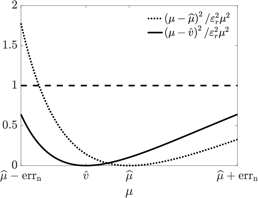
The common case of estimating the integral itself, p=1p=1 and v⁡(μ)=μv(\mu)=\mu, is illustrated in Table 1. This includes i) an absolute error criterion (see (1)), ii) a relative error criterion, and iii) a hybrid error criterion that is satisfied when either the absolute or relative error tolerances are satisfied. Note that v^\hat{v} is not necessarily equal to μ^n\hat{\mu}_{n}. For a pure relative error criterion, v^\hat{v} represents a shrinkage of the sample mean towards zero. Fig. 4 illustrates how the optimal choice of v^\hat{v} may satisfy (13), when v^=μ^\hat{v}=\hat{\mu} does not.

Table 1: Examples of the tolerance function in (13) and the optimal approximation to the integral when p=1p=1 and v⁡(μ)=μv(\mu)=\mu.
Kindtol​(μ,v^,εa,εr)Optimal ​v^Optimal tol​(μ,v^,εa,εr)​[−1​e​x]​Absolute​εr=0(μ−v^)2εa2μ^nerrn2εa2​[2​e​x]​Relative​εa=0(μ−v^)2εr2​μ2max⁡(μ^n2−errn2,0)μ^nerrn2εr2​max⁡(μ^n2,errn2)​[2​e​x]​Hybrid(μ−v^)2max⁡(εa2,ϵr2​μ2)see (18)see (19)\begin{array}[]{p{1.2cm}@{\quad}c@{\quad}c@{\quad}c}Kind&\textup{tol}(\mu,\hat{v},\varepsilon_{\textrm{a}},\varepsilon_{\textrm{r}})&\text{Optimal }\hat{v}&\hfil\text{Optimal }\textup{tol}(\mu,\hat{v},\varepsilon_{\textrm{a}},\varepsilon_{\textrm{r}})\hfil\lx@intercol\lx@intercol[-1ex]\lx@intercol\text{Absolute}\newline \text{$\varepsilon_{\textrm{r}}=0$}&\displaystyle\frac{(\mu-\hat{v})^{2}}{\varepsilon_{\textrm{a}}^{2}}&\widehat{\mu}_{n}&\displaystyle\frac{\textup{err}_{n}^{2}}{\varepsilon_{\textrm{a}}^{2}}[2ex]\vskip-12.91663pt\text{Relative}\newline \text{$\varepsilon_{\textrm{a}}=0$}&\displaystyle\frac{(\mu-\hat{v})^{2}}{\varepsilon_{\textrm{r}}^{2}\mu^{2}}&\displaystyle\frac{\max(\widehat{\mu}_{n}^{2}-\textup{err}_{n}^{2},0)}{\widehat{\mu}_{n}}&\displaystyle\frac{\textup{err}_{n}^{2}}{\varepsilon^{2}_{r}\max(\widehat{\mu}_{n}^{2},\textup{err}_{n}^{2})}[2ex]\text{Hybrid}&\displaystyle\frac{(\mu-\hat{v})^{2}}{\max(\varepsilon_{\textrm{a}}^{2},\epsilon_{r}^{2}\mu^{2})}&\text{see \eqref{FTD:eq:vhatveqmu}}&\text{see \eqref{FTD:eq:tolveqmu}}\end{array}
Refer to caption
Figure 4: Example of v⁡(μ)=μv(\mu)=\mu with the relative error criterion, i.e. εa=0\varepsilon_{\textrm{a}}=0. For the optimal choice of v^\hat{v}, supμ∈[μ^n−errn,μ^n+errn]tol​(μ,v^,εa,εr)<1<supμ∈[μ^n−errn,μ^n+errn]tol​(μ,μ^n,εa,εr)\sup_{\mu\in[\widehat{\mu}_{n}-\textup{err}_{n},\widehat{\mu}_{n}+\textup{err}_{n}]}\textup{tol}(\mu,\hat{v},\varepsilon_{\textrm{a}},\varepsilon_{\textrm{r}})<1<\sup_{\mu\in[\widehat{\mu}_{n}-\textup{err}_{n},\widehat{\mu}_{n}+\textup{err}_{n}]}\textup{tol}(\mu,\widehat{\mu}_{n},\varepsilon_{\textrm{a}},\varepsilon_{\textrm{r}}).

Define v±v_{\pm} as the extreme values of v⁡(μ)v(\mu) for 𝝁^\widehat{\bm{\mu}} satisfying the given error bound:

v−=inf𝝁∈Ω∩[𝝁^n−errn,𝝁^n+errn]v⁡(𝝁),v+=sup𝝁∈Ω∩[𝝁^n−errn,𝝁^n+errn]v⁡(𝝁)v_{-}=\inf_{{\bm{\mu}}\in\Omega\cap[\widehat{{\bm{\mu}}}_{n}-\textbf{{err}}_{n},\widehat{{\bm{\mu}}}_{n}+\textbf{{err}}_{n}]}v({\bm{\mu}}),\qquad v_{+}=\sup_{{\bm{\mu}}\in\Omega\cap[\widehat{{\bm{\mu}}}_{n}-\textbf{{err}}_{n},\widehat{{\bm{\mu}}}_{n}+\textbf{{err}}_{n}]}v({\bm{\mu}}) (14)

Then the following criterion is equivalent to (13):

supv−≤v′≤v+tol​(v′,v^,εa,εr)≤1.\sup_{v_{-}\leq v^{\prime}\leq v_{+}}\textup{tol}(v^{\prime},\hat{v},\varepsilon_{\textrm{a}},\varepsilon_{\textrm{r}})\leq 1. (15)

We claim that the optimal value of the estimated integral, i.e., the value of v^\hat{v} satisfying (15), is

v^\displaystyle\hat{v} =v−​max⁡(εa,εr​|v+|)+v+​max⁡(εa,εr​|v−|)max⁡(εa,εr​|v+|)+max⁡(εa,εr​|v−|)\displaystyle=\frac{v_{-}\max(\varepsilon_{\textrm{a}},\varepsilon_{\textrm{r}}\left\lvert v_{+}\right\rvert)+v_{+}\max(\varepsilon_{\textrm{a}},\varepsilon_{\textrm{r}}\left\lvert v_{-}\right\rvert)}{\max(\varepsilon_{\textrm{a}},\varepsilon_{\textrm{r}}\left\lvert v_{+}\right\rvert)+\max(\varepsilon_{\textrm{a}},\varepsilon_{\textrm{r}}\left\lvert v_{-}\right\rvert)} (16a)
={v−+v+2,εr​|v±|≤εa,vs​[εa+v−s​εr​sign​(vs)]εa+εr​|vs|,εr|v−s|≤εa<εr|vs|,s∈{+,−},|v+​v−|​[sign​(v+)+sign​(v−)]|v+|+|v−|,εa<εr​|v±|.\displaystyle=\begin{cases}\displaystyle\frac{v_{-}+v_{+}}{2},&\varepsilon_{\textrm{r}}\left\lvert v_{\pm}\right\rvert\leq\varepsilon_{\textrm{a}},\\[6.45831pt] \displaystyle\frac{v_{s}[\varepsilon_{\textrm{a}}+v_{-s}\varepsilon_{\textrm{r}}\textup{sign}(v_{s})]}{\varepsilon_{\textrm{a}}+\varepsilon_{\textrm{r}}\left\lvert v_{s}\right\rvert},&\varepsilon_{\textrm{r}}\left\lvert v_{-s}\right\rvert\leq\varepsilon_{\textrm{a}}<\varepsilon_{\textrm{r}}\left\lvert v_{s}\right\rvert,\ s\in\{+,-\},\\[6.45831pt] \displaystyle\frac{\left\lvert v_{+}v_{-}\right\rvert[\textup{sign}(v_{+})+\textup{sign}(v_{-})]}{\left\lvert v_{+}\right\rvert+\left\lvert v_{-}\right\rvert},&\varepsilon_{\textrm{a}}<\varepsilon_{\textrm{r}}\left\lvert v_{\pm}\right\rvert.\end{cases} (16b)

From (16a) it follows that v^∈[v−,v+]\hat{v}\in[v_{-},v_{+}]. Moreover, by (16b) v^\hat{v} is a shrinkage estimator: it is either zero or has the same sign as (v−+v+)/2(v_{-}+v_{+})/2, and its magnitude is no greater than |(v−+v+)/2|\left\lvert(v_{-}+v_{+})/2\right\rvert. Our improved GAIL algorithms cubSobol_g and cubLattice_g, which are under development, are summarized in the following theorem.

Theorem 3.1

Let our goal be the computation of v⁡(𝛍)v({\bm{\mu}}), as described at the beginning of this section. Let the tolerance function be defined as in (13b), let the extreme possible values of v⁡(𝛍)v({\bm{\mu}}) be defined as in (14), and let the approximation to v⁡(𝛍)v({\bm{\mu}}) be defined in terms of 𝛍^n\widehat{{\bm{\mu}}}_{n} and errn\textbf{{err}}_{n} as in (16). Then, v^\hat{v} is the optimal approximation to v⁡(𝛍)v({\bm{\mu}}), and the tolerance function for this optimal choice is given as follows:

infv^′sup𝝁∈Ω∩[𝝁^n−errn,𝝁^n+errn]tol​(v⁡(𝝁),v^′,εa,εr)\displaystyle\hskip-34.44434pt\inf_{\hat{v}^{\prime}}\sup_{{\bm{\mu}}\in\Omega\cap[\widehat{{\bm{\mu}}}_{n}-\textbf{{err}}_{n},\widehat{{\bm{\mu}}}_{n}+\textbf{{err}}_{n}]}\textup{tol}(v({\bm{\mu}}),\hat{v}^{\prime},\varepsilon_{\textrm{a}},\varepsilon_{\textrm{r}})
=infv^′supv−≤v′≤v+tol​(v′,v^′,εa,εr)\displaystyle=\inf_{\hat{v}^{\prime}}\sup_{v_{-}\leq v^{\prime}\leq v_{+}}\textup{tol}(v^{\prime},\hat{v}^{\prime},\varepsilon_{\textrm{a}},\varepsilon_{\textrm{r}}) (17a)
=supv−≤v′≤v+tol​(v′,v^,εa,εr)\displaystyle=\sup_{v_{-}\leq v^{\prime}\leq v_{+}}\textup{tol}(v^{\prime},\hat{v},\varepsilon_{\textrm{a}},\varepsilon_{\textrm{r}}) (17b)
=tol​(v±,v^,εa,εr)\displaystyle=\textup{tol}(v_{\pm},\hat{v},\varepsilon_{\textrm{a}},\varepsilon_{\textrm{r}}) (17c)
=(v+−v−)2[max⁡(εa,εr​|v+|)+max⁡(εa,εr​|v−|)]2.\displaystyle=\frac{(v_{+}-v_{-})^{2}}{[\max(\varepsilon_{\textrm{a}},\varepsilon_{\textrm{r}}\left\lvert v_{+}\right\rvert)+\max(\varepsilon_{\textrm{a}},\varepsilon_{\textrm{r}}\left\lvert v_{-}\right\rvert)]^{2}}. (17d)

By optimal, we mean that the infimum in (17a) is satisfied by v^\hat{v} as claimed in (17b). Moreover, it is shown that the supremum in (17b) is obtained simultaneously at v+v_{+} and v−v_{-}.

Our new adaptive quasi-Monte Carlo cubature algorithms increase n=2mn=2^{m} by incrementing mm by one until the right side of (17d) is no larger than one. The resulting v^\hat{v} then satisfies the error criterion tol​(v⁡(𝛍),v^,εa,εr)≤1\textup{tol}(v({\bm{\mu}}),\hat{v},\varepsilon_{\textrm{a}},\varepsilon_{\textrm{r}})\leq 1.

Proof

The gist of the proof is to establish the equalities in (17). Equality (17d) follows from the definition of v^\hat{v} and v±v_{\pm}. Equality (17c) is proven next, and (17b) is proven after that. Equality (17a) follows from definition (14).

The derivative of tol​(⋅,v^,εa,εr)\textup{tol}(\cdot,\hat{v},\varepsilon_{\textrm{a}},\varepsilon_{\textrm{r}}) is

∂tol​(v′,v^,εa,εr)∂v′={2​(v′−v^)εa2,|v′|<εaεr,2​(v′−v^)​v^εr2​v′3,|v′|>εaεr.\frac{\partial\textup{tol}(v^{\prime},\hat{v},\varepsilon_{\textrm{a}},\varepsilon_{\textrm{r}})}{\partial v^{\prime}}=\begin{cases}\displaystyle\frac{2(v^{\prime}-\hat{v})}{\varepsilon_{\textrm{a}}^{2}},&\displaystyle\left\lvert v^{\prime}\right\rvert<\frac{\varepsilon_{\textrm{a}}}{\varepsilon_{\textrm{r}}},\\[8.61108pt] \displaystyle\frac{2(v^{\prime}-\hat{v})\hat{v}}{\varepsilon_{\textrm{r}}^{2}v^{\prime 3}},&\displaystyle\left\lvert v^{\prime}\right\rvert>\frac{\varepsilon_{\textrm{a}}}{\varepsilon_{\textrm{r}}}.\end{cases}

The sign of this derivative is shown in Fig. 5. For either εr​|v±|≤εa\varepsilon_{\textrm{r}}\left\lvert v_{\pm}\right\rvert\leq\varepsilon_{\textrm{a}} or εa≤εr​|v±|\varepsilon_{\textrm{a}}\leq\varepsilon_{\textrm{r}}\left\lvert v_{\pm}\right\rvert, the only critical point in [v−,v+][v_{-},v_{+}] is v′=v^v^{\prime}=\hat{v}, where the tolerance function vanishes. Thus, the maximum value of the tolerance function always occurs at the boundaries of the interval. For εr​|v−s|≤εa<εr​|vs|\varepsilon_{\textrm{r}}\left\lvert v_{-s}\right\rvert\leq\varepsilon_{\textrm{a}}<\varepsilon_{\textrm{r}}\left\lvert v_{s}\right\rvert, s∈{+,−}s\in\{+,-\}, there is also a critical point at v′=sign​(vs)​εa/εrv^{\prime}=\textup{sign}(v_{s})\varepsilon_{\textrm{a}}/\varepsilon_{\textrm{r}}. However, since vsv_{s} and v^\hat{v} have the same sign (see (16b)), the partial derivative of the tolerance function with respect to v′v^{\prime} does not change sign at this critical point. Hence, the maximum value of the tolerance function still occurs at the boundaries of the interval, and (17c) is established.

Refer to caption
Figure 5: The sign of ∂tol​(v′,v^,εa,εr)/∂v′\partial\textup{tol}(v^{\prime},\hat{v},\varepsilon_{\textrm{a}},\varepsilon_{\textrm{r}})/\partial v^{\prime}.

To prove assertion (17b), consider v^′\hat{v}^{\prime}, some alternative to v^\hat{v}. Then

tol​(v±,v^′,εa,εr)−tol​(v±,v^,εa,εr)\displaystyle\textup{tol}(v_{\pm},\hat{v}^{\prime},\varepsilon_{\textrm{a}},\varepsilon_{\textrm{r}})-\textup{tol}(v_{\pm},\hat{v},\varepsilon_{\textrm{a}},\varepsilon_{\textrm{r}}) =(v±−v^′)2−(v±−v^)2max⁡(εa2,εr2​v±2)\displaystyle=\frac{(v_{\pm}-\hat{v}^{\prime})^{2}-(v_{\pm}-\hat{v})^{2}}{\max(\varepsilon_{\textrm{a}}^{2},\varepsilon_{\textrm{r}}^{2}v_{\pm}^{2})}
=(v^′−v^−2​v±)​(v^′−v^)max⁡(εa2,εr2​v±2).\displaystyle=\frac{(\hat{v}^{\prime}-\hat{v}-2v_{\pm})(\hat{v}^{\prime}-\hat{v})}{\max(\varepsilon_{\textrm{a}}^{2},\varepsilon_{\textrm{r}}^{2}v_{\pm}^{2})}.

This difference is positive for the ++ sign if v^′∈(−∞,v^)\hat{v}^{\prime}\in(-\infty,\hat{v}) and positive for the −- sign if v^′∈(v^,∞)\hat{v}^{\prime}\in(\hat{v},\infty). Thus, the proof of Theorem 3.1 is complete.

We return to the special case of v⁡(μ)=μv(\mu)=\mu. The following corollary interprets Theorem 3.1 for this case, and the theorem that follows extends the computational cost upper bound in (12) for these new quasi-Monte Carlo cubature algorithms.

Corollary 1

For p=1p=1 and v⁡(μ)=μv(\mu)=\mu, it follows that v±=μn±errnv_{\pm}=\mu_{n}\pm\textup{err}_{n},

v^=(μ^n−errn)​max⁡(εa,εr​|μ^n+errn|)+(μ^n+errn)​max⁡(εa,εr​|μ^n−errn|)max⁡(εa,εr​|μ^n+errn|)+max⁡(εa,εr​|μ^n−errn|),\hat{v}=\frac{(\widehat{\mu}_{n}-\textup{err}_{n})\max(\varepsilon_{\textrm{a}},\varepsilon_{\textrm{r}}\left\lvert\widehat{\mu}_{n}+\textup{err}_{n}\right\rvert)+(\widehat{\mu}_{n}+\textup{err}_{n})\max(\varepsilon_{\textrm{a}},\varepsilon_{\textrm{r}}\left\lvert\widehat{\mu}_{n}-\textup{err}_{n}\right\rvert)}{\max(\varepsilon_{\textrm{a}},\varepsilon_{\textrm{r}}\left\lvert\widehat{\mu}_{n}+\textup{err}_{n}\right\rvert)+\max(\varepsilon_{\textrm{a}},\varepsilon_{\textrm{r}}\left\lvert\widehat{\mu}_{n}-\textup{err}_{n}\right\rvert)}, (18)
supμ^n−errn≤μ≤μ^n+errntol​(μ,v^,εa,εr)=4​errn2[max⁡(εa,εr​|μ^n+errn|)+max⁡(εa,εr​|μ^n−errn|)]2.\sup_{\widehat{\mu}_{n}-\textup{err}_{n}\leq\mu\leq\widehat{\mu}_{n}+\textup{err}_{n}}\textup{tol}(\mu,\hat{v},\varepsilon_{\textrm{a}},\varepsilon_{\textrm{r}})\\ =\frac{4\textup{err}_{n}^{2}}{[\max(\varepsilon_{\textrm{a}},\varepsilon_{\textrm{r}}\left\lvert\widehat{\mu}_{n}+\textup{err}_{n}\right\rvert)+\max(\varepsilon_{\textrm{a}},\varepsilon_{\textrm{r}}\left\lvert\widehat{\mu}_{n}-\textup{err}_{n}\right\rvert)]^{2}}. (19)
Theorem 3.2

For the special case described in Corollary 1, the computational cost of obtaining an approximation to the integral μ\mu satisfying the generalized error criterion tol​(μ,v^,εa,εr)≤1\textup{tol}(\mu,\hat{v},\varepsilon_{\textrm{a}},\varepsilon_{\textrm{r}})\leq 1 according to the adaptive quasi-Monte Carlo cubature algorithm described in Theorem 3.1 is 𝒪⁡([$(f)+m∗]​2m∗){\mathcal{O}}\bigl([\$(f)+m^{*}]2^{m^{*}}\bigr), where

m∗:=min{m≥ℓ∗+r:(1+εr)ω^​(m)​ω̊​(r)1−ω^​(r)​ω̊​(r)[1+ω^(r)ω̊(r)]Sm−r(f)≤max(εa,εr|μ|)}.m^{*}:=\min\left\{m\geq\ell_{*}+r:\;\right.\\ \left.(1+\varepsilon_{\textrm{r}})\frac{\widehat{\omega}(m)\mathring{\omega}(r)}{1-\widehat{\omega}(r)\mathring{\omega}(r)}[1+\widehat{\omega}(r)\mathring{\omega}(r)]S_{m-r}(f)\leq\max(\varepsilon_{\textrm{a}},\varepsilon_{\textrm{r}}\left\lvert\mu\right\rvert)\right\}.
Proof

For each n=2mn=2^{m}, we know that our algorithm produces μ^n\widehat{\mu}_{n} and errn\textup{err}_{n} satisfying μ^n−errn≤μ≤μ^n+errn\widehat{\mu}_{n}-\textup{err}_{n}\leq\mu\leq\widehat{\mu}_{n}+\textup{err}_{n}. This implies that

max⁡(εa,εr​|μ^n+errn|)+max⁡(εa,εr​|μ^n−errn|)≥2​max⁡(εa,εr​|μ|)−2​εr​errn.\max(\varepsilon_{\textrm{a}},\varepsilon_{\textrm{r}}\left\lvert\widehat{\mu}_{n}+\textup{err}_{n}\right\rvert)+\max(\varepsilon_{\textrm{a}},\varepsilon_{\textrm{r}}\left\lvert\widehat{\mu}_{n}-\textup{err}_{n}\right\rvert)\geq 2\max(\varepsilon_{\textrm{a}},\varepsilon_{\textrm{r}}\left\lvert\mu\right\rvert)-2\varepsilon_{\textrm{r}}\textup{err}_{n}.

Thus, the right hand side of (19) must be no greater than one if

errn≤max⁡(εa,εr​|μ|)1+εr.\textup{err}_{n}\leq\frac{\max(\varepsilon_{\textrm{a}},\varepsilon_{\textrm{r}}\left\lvert\mu\right\rvert)}{1+\varepsilon_{\textrm{r}}}.

Applying the logic that leads to (12) completes the proof.

The cost upper bound depends on various parameters as one would expect. The computational cost may increase if

  • •

    εa\varepsilon_{\textrm{a}} decreases,

  • •

    εr\varepsilon_{\textrm{r}} decreases,

  • •

    |μ|\left\lvert\mu\right\rvert decreases,

  • •

    the Fourier coefficients of the integrand increase, or

  • •

    the cone 𝒞\mathcal{C} expands because ℓ∗\ell_{*}, ω^\widehat{\omega}, or ω̊\mathring{\omega} increase.

4 Numerical Implementation

The algorithm described here is intended to be released in the next release of GAIL [2] as cubSobol_g and cubLattice_g, coded in MATLAB. These two functions use the Sobol’ sequences provided by MATLAB 2017a [26] and the lattice generator exod2_base2_m20.txt from Dirk Nuyens’ website [20], respectively. Our algorithm sets its default parameters as follows:

ℓ∗=6,r=4,ℭ⁡(m)=5×2−m.\ell_{*}=6,\qquad r=4,\qquad{\mathfrak{C}}(m)=5\times 2^{-m}. (20)

These choices are based on experience and are used in the examples below. A larger ℓ∗\ell_{*} allows the Fourier coefficients of the integrand to behave erratically over a larger initial segment of wavenumbers. A larger rr decreases the impact of aliasing in estimating the true Fourier coefficients by their discrete analogues. Increasing ℓ∗\ell_{*} or rr increases 2ℓ∗+r2^{\ell_{*}+r}, the minimum number of sample points used by the algorithms. The inputs to the algorithms are

  • •

    a black-box pp-vector function 𝒇{\bm{f}}, such that 𝝁=𝔼⁡[𝒇⁡(𝑿)]{\bm{\mu}}=\mathbb{E}[{\bm{f}}({\bm{X}})] for 𝑿∼𝒰​[0,1]d{\bm{X}}\sim{\mathcal{U}}[0,1]^{d},

  • •

    a solution function v:ℝp→ℝv:{\mathbb{R}}^{p}\to{\mathbb{R}},

  • •

    functions for computing v±v_{\pm} as described in (14),

  • •

    an absolute error tolerance, εa\varepsilon_{\textrm{a}}, and

  • •

    a relative error tolerance εr\varepsilon_{\textrm{r}}.

The algorithm increases mm incrementally until the right side of (17d) does not exceed one. At this point the algorithm returns v^\hat{v} as given by (16).

Example 1

We illustrate the hybrid error criterion by estimating multivariate normal probabilities for a distribution with mean 𝟎{\bm{0}} and covariance matrix Σ\mathsf{\Sigma}:

v(μ)=μ=ℙ[𝒂≤𝑿≤𝒃]=∫[𝒂,𝒃]e−𝒙TΣ−1𝒙/2(2​π)d/2​|Σ|1/2d𝒙.v(\mu)=\mu=\mathbb{P}\left[{\bm{a}}\leq{\bm{X}}\leq{\bm{b}}\right]=\int_{[{\bm{a}},{\bm{b}}]}\frac{\mathrm{e}^{-{\bm{x}}^{T}\mathsf{\Sigma}^{-1}{\bm{x}}/2}}{(2\pi)^{d/2}\left\lvert\mathsf{\Sigma}\right\rvert^{1/2}}\,\mathrm{d}{\bm{x}}. (21)

The transformation proposed by Genz [5] is used write this as an integral over the d−1d-1 dimensional unit cube. As discussed in [5, 9], when 𝐚=−∞{\bm{a}}=-\bm{\infty}, Σi​j=σ\mathsf{\Sigma}_{ij}=\sigma if i≠ji\neq j, and Σi​i=1\mathsf{\Sigma}_{ii}=1, the exact value of (21) reduces to a 1-dimensional integral that can be accurately estimated by a standard quadrature rule. This value is taken to be the true μ\mu.

We perform 10001000 adaptive integrations: 500500 using our cubature rule based on randomly scrambled and digitally shifted Sobol’ sequences (cubSobol_g) and 500500 using our cubature rule based on randomly shifted rank-1 lattice node sequences, (cubLattice_g). Default parameters are used. For each case we choose σ∼𝒰⁡[0,1]\sigma\sim\mathcal{U}[0,1], dimension d=⌊500D⌋d=\lfloor 500^{D}\rfloor with D∼𝒰⁡[0,1]D\sim\mathcal{U}[0,1], and 𝐛∼𝒰​[0,d]d{\bm{b}}\sim\mathcal{U}[0,\sqrt{d}]^{d}. The dependence of 𝐛{\bm{b}} on the dimension of the problem ensures that the estimated probabilities are of the same order of magnitude for all dd. Otherwise, the higher the dimension, the smaller the value of the probabilities the test would be estimating. The execution time and tol​(μ,v^,0.01,0.05)\textup{tol}(\mu,\hat{v},0.01,0.05) are shown in Fig. 6.

Refer to caption
Refer to caption
Figure 6: On the left, 500500 integration results using scrambled and digitally shifted Sobol’ sequences, cubSobol_g. On the right, tolerance values and computation times of integrating 500500 multivariate normal probabilities using randomly shifted rank-1 lattice node sequences, cubLattice_g. If an integrand is in 𝒞\mathcal{C}, its dot must lie to the left of the vertical dot-dashed line denoting tol​(μ,v^,0.01,0.05)=1\textup{tol}(\mu,\hat{v},0.01,0.05)=1. The solid and dashed curves represent the empirical distributions of tolerance values and times respectively.

Satisfying the error criterion is equivalent to having tol​(μ,v^,0.01,0.05)≤1\textup{tol}(\mu,\hat{v},0.01,0.05)\leq 1, which happens in every case. A very small value of tol​(μ,v^,0.01,0.05)\textup{tol}(\mu,\hat{v},0.01,0.05) means that the approximation is much more accurate than required, which may be due to coincidence or due to the minimum sample size used, n=210n=2^{10}. In Fig. 6 the error tolerances are fixed and do not affect the computation time. However, the computation time does depend on the dimension, dd, since higher dimensional problems tend to be harder to solve. The performances of cubSobol_g and cubLattice_g are similar.

Example 2

Sobol’ indices [24, 25], which arise in uncertainty quantification, depend on more than one integral. Suppose that one is interested in how an output, Y:=g⁡(𝐗)Y:=g({\bm{X}}) depends on the input 𝐗∼𝒰​[0,1]d{\bm{X}}\sim\mathcal{U}[0,1]^{d}, and gg has a complicated or unknown structure. For example, gg might be the output of a computer simulation. For any coordinate indexed by j=1,…,dj=1,\dots,d, the normalized closed first-order Sobol’ index for coordinate jj, commonly denoted as τ¯j2/σ2\underline{\tau}_{j}^{2}/\sigma^{2}, involves three integrals:

v(𝝁):=μ1μ2−μ32,μ1:=∫[0,1)2​d[g(𝒙j:𝒙′−j)−g(𝒙′)]g(𝒙)d𝒙d𝒙′,\displaystyle v({\bm{\mu}}):=\frac{\mu_{1}}{\mu_{2}-\mu_{3}^{2}},\qquad\mu_{1}:=\int_{[0,1)^{2d}}[g({\bm{x}}_{j}:{{\bm{x}}^{\prime}}_{-j})-g({\bm{x}}^{\prime})]g({\bm{x}})\,\mathrm{d}{\bm{x}}\,\mathrm{d}{\bm{x}}^{\prime}, (22a)
μ2:=∫[0,1)dg(𝒙)2d𝒙,μ3:=∫[0,1)dg(𝒙)d𝒙.\displaystyle\mu_{2}:=\int_{[0,1)^{d}}g({\bm{x}})^{2}\,\mathrm{d}{\bm{x}},\qquad\mu_{3}:=\int_{[0,1)^{d}}g({\bm{x}})\,\mathrm{d}{\bm{x}}. (22b)

Here, (𝐱j:𝐱′−j)∈[0,1)d({\bm{x}}_{j}:{{\bm{x}}^{\prime}}_{-j})\in[0,1)^{d} denotes a point whose rthr^{\text{th}} coordinate is xrx_{r} if r=jr=j, and xr′x^{\prime}_{r} otherwise. By definition, the value of these normalized indices must lie between 00 and 11, and both the numerator and denominator in the expression for v⁡(𝛍)v({\bm{\mu}}) are non-negative. Therefore, the domain of the function vv is Ω:={𝛍∈[0,∞)3:0≤μ1≤μ2−μ32}\Omega:=\{{\bm{\mu}}\in[0,\infty)^{3}:0\leq\mu_{1}\leq\mu_{2}-\mu_{3}^{2}\}. Thus, given 𝛍^n\widehat{{\bm{\mu}}}_{n} and errn\textbf{{err}}_{n}, the values of v±v_{\pm} defined in (14) are

v±={0,μn,1±errn,1≤0,1,μn,1±errn,1>max⁡(0,μn,2∓errn,2−(μn,3±errn,3)2),μn,1±errn,1μn,2∓errn,2−(μn,3±errn,3)2,otherwise.v_{\pm}=\begin{cases}0,\qquad\mu_{n,1}\pm\textup{err}_{n,1}\leq 0,\\ 1,\qquad\mu_{n,1}\pm\textup{err}_{n,1}>\max\bigl(0,\mu_{n,2}\mp\textup{err}_{n,2}-(\mu_{n,3}\pm\textup{err}_{n,3})^{2}\bigr),\\ \displaystyle\frac{\mu_{n,1}\pm\textup{err}_{n,1}}{\mu_{n,2}\mp\textup{err}_{n,2}-(\mu_{n,3}\pm\textup{err}_{n,3})^{2}},\qquad\text{otherwise}.\end{cases} (23)

We estimate the first-order Sobol’ indices of the test function in Bratley et al. [1] using randomly scrambled and digitally shifted Sobol’ sequences and the same algorithm parameters as in Ex. 1:

g⁡(𝑿)=∑i=16(−1)i​∏j=1i𝑿j.g({\bm{X}})=\sum_{i=1}^{6}(-1)^{i}\prod_{j=1}^{i}{\bm{X}}_{j}.
j123456n8​1924​0961​0241​0241​0241​024v0.65290.17910.03700.01330.00150.0015v^0.64950.17940.03360.01340.00100.0016v⁡(𝝁^n)0.64020.17000.03360.01340.00090.0016tol​(v,v^,5×10−3,0)0.44690.00240.46460.00030.01120.0002tol​(v,v⁡(𝝁^n),5×10−3,0)6.46233.33130.47650.00020.01130.0002\begin{array}[]{ r | ccccccc }j&1&2&3&4&5&6\\ n&8~192&4~096&1~024&1~024&1~024&1~024\\ v&0.6529&0.1791&0.0370&0.0133&0.0015&0.0015\\ \hat{v}&0.6495&0.1794&0.0336&0.0134&0.0010&0.0016\\ v(\widehat{{\bm{\mu}}}_{n})&0.6402&0.1700&0.0336&0.0134&0.0009&0.0016\\ \textup{tol}(v,\hat{v},5\times 10^{-3},0)&0.4469&0.0024&0.4646&0.0003&0.0112&0.0002\\ \textup{tol}(v,v(\widehat{{\bm{\mu}}}_{n}),5\times 10^{-3},0)&6.4623&3.3313&0.4765&0.0002&0.0113&0.0002\end{array}

The value of nn chosen by our adaptive algorithm and the actual value of the tolerance function, tol​(v,v^,5×10−3,0)\textup{tol}(v,\hat{v},5\times 10^{-3},0), are shown. Since none of those tolerance values exceed one, our algorithm correctly provides v^\hat{v} for each coordinate jj. In the last row above, we replaced our optimal v^\hat{v} by v⁡(𝛍^n)v(\widehat{{\bm{\mu}}}_{n}) for the same nn as returned by our algorithm. Interestingly, this approximation to the Sobol’ indices, while perhaps intuitive, does not satisfy the absolute error criterion because sometimes tol​(v,v⁡(𝛍^n),5×10−3,0)\textup{tol}(v,v(\widehat{{\bm{\mu}}}_{n}),5\times 10^{-3},0) exceeds one. This reflects how v⁡(𝛍^n)v(\widehat{{\bm{\mu}}}_{n}) differs from vv much more than v^\hat{v} does. An extensive study on how to estimate first-order and total effect Sobol’ indices using the automatic quasi-Monte Carlo cubature is provided in [14].

5 Control Variates

The results in this section mainly follow the work of Da Li [16]. Control variates are commonly used to improve the efficiency of IID Monte Carlo integration. If one chooses a vector of functions 𝒈:[0,1)d→ℝq{\bm{g}}:[0,1)^{d}\to{\mathbb{R}}^{q} for which 𝝁𝒈:=∫[0,1)d𝒈(𝒙)d𝒙{\bm{\mu}}_{\bm{g}}:=\int_{[0,1)^{d}}{\bm{g}}({\bm{x}})\,\mathrm{d}{\bm{x}} is known, then

μ:=∫[0,1)df(𝒙)d𝒙=∫[0,1)dh𝜷(𝒙)d𝒙,where h𝜷(𝒙):=f(𝒙)+𝜷T(𝝁𝒈−𝒈(𝒙)),\mu:=\int_{[0,1)^{d}}f({\bm{x}})\,\mathrm{d}{\bm{x}}=\int_{[0,1)^{d}}h_{{\bm{\beta}}}({\bm{x}})\,\mathrm{d}{\bm{x}},\qquad\text{where }h_{{\bm{\beta}}}({\bm{x}}):=f({\bm{x}})+{\bm{\beta}}^{T}({\bm{\mu}}_{\bm{g}}-{\bm{g}}({\bm{x}})),

for any choice of 𝜷{\bm{\beta}}. The goal is to choose an optimal 𝜷{\bm{\beta}} to make

μ^𝜷,n:=1n​∑i=0n−1h𝜷​(𝒙i)\widehat{\mu}_{{\bm{\beta}},n}:=\frac{1}{n}\sum_{i=0}^{n-1}h_{{\bm{\beta}}}({\bm{x}}_{i})

sufficiently close to μ\mu with the least expense, nn, possible.

If 𝒙0,𝒙1,…{\bm{x}}_{0},{\bm{x}}_{1},\ldots are IID 𝒰[0,1)d{\mathcal{U}}[0,1)^{d}, then μ^𝜷,n\widehat{\mu}_{{\bm{\beta}},n} is an unbiased estimator for μ\mu for any choice of 𝜷{\bm{\beta}}, and the variance of the control variates estimator may be expressed as

var​(μ^𝜷,n)=var​(h𝜷​(𝒙0))n=1n​∑κ=1∞|f^κ−𝜷T​𝒈^κ|2,\textup{var}(\widehat{\mu}_{{\bm{\beta}},n})=\frac{\textup{var}(h_{{\bm{\beta}}}({\bm{x}}_{0}))}{n}=\frac{1}{n}\sum_{\kappa=1}^{\infty}\left\lvert\hat{f}_{\kappa}-{\bm{\beta}}^{T}\hat{{\bm{g}}}_{\kappa}\right\rvert^{2},

where 𝒈^κ\hat{{\bm{g}}}_{\kappa} are the Fourier coefficients of 𝒈{\bm{g}}. Since 𝜷T​𝝁𝒈{\bm{\beta}}^{T}{\bm{\mu}}_{\bm{g}} is constant, it does not enter into the calculation of the variance. The optimal choice of 𝜷{\bm{\beta}}, which minimizes var​(μ^𝜷,n)\textup{var}(\widehat{\mu}_{{\bm{\beta}},n}), is

𝜷MC=cov​(f⁡(𝒙0),𝒈⁡(𝒙0))var​(𝒈​(𝒙0)).{\bm{\beta}}_{\textup{MC}}=\frac{\textup{cov}\bigl(f({\bm{x}}_{0}),{\bm{g}}({\bm{x}}_{0})\bigr)}{\textup{var}\bigl({\bm{g}}({\bm{x}}_{0})\bigr)}.

Although 𝜷MC{\bm{\beta}}_{\textup{MC}} cannot be computed exactly, it may be well approximated in terms of sample estimates of the quantities on the right hand side.

However, if 𝒙0,𝒙1,…{\bm{x}}_{0},{\bm{x}}_{1},\ldots are the points described in Sec. 2, then the error depends on only some of the Fourier coefficients, and (5) and (9) lead to

|μ−μ^𝜷,n|≤∑λ=1∞|f^λ​2m−𝜷T​𝒈^λ​2m|≤ω^​(m)​ω̊​(r)1−ω^​(r)​ω̊​(r)​S~m−r,m​(f−𝜷T​𝒈),provided ​f−𝜷T​𝒈∈𝒞.\left\lvert\mu-\widehat{\mu}_{{\bm{\beta}},n}\right\rvert\leq\sum_{\lambda=1}^{\infty}\left\lvert\hat{f}_{\lambda 2^{m}}-{\bm{\beta}}^{T}\hat{{\bm{g}}}_{\lambda 2^{m}}\right\rvert\leq\frac{\widehat{\omega}(m)\mathring{\omega}(r)}{1-\widehat{\omega}(r)\mathring{\omega}(r)}\widetilde{S}_{m-r,m}(f-{\bm{\beta}}^{T}{\bm{g}}),\\ \text{provided }f-{\bm{\beta}}^{T}{\bm{g}}\in{\mathcal{C}}. (24)

Assuming that f−𝜷T​𝒈∈𝒞f-{\bm{\beta}}^{T}{\bm{g}}\in{\mathcal{C}} for all 𝜷{\bm{\beta}}, it makes sense to choose 𝜷{\bm{\beta}} to minimize the rightmost term. There seems to be some advantage to choose 𝜷{\bm{\beta}} based on S~m−r,m​(f−𝜷T​𝒈),…,S~m,m​(f−𝜷T​𝒈)\widetilde{S}_{m-r,m}(f-{\bm{\beta}}^{T}{\bm{g}}),\ldots,\widetilde{S}_{m,m}(f-{\bm{\beta}}^{T}{\bm{g}}). Our experience suggests that this strategy makes 𝜷{\bm{\beta}} less dependent on the fluctuations of the discrete Fourier coefficients over a small range of wave numbers. In summary,

𝜷qMC=argmin𝒃∑t=0rS~m−t,m(f−𝒃T𝒈)=argmin𝒃∑κ=⌊2m−r−1⌋2m−1|f~m,κ−𝒃T𝒈~m,κ|.{\bm{\beta}}_{\textup{qMC}}=\operatorname*{argmin}_{\bm{b}}\sum_{t=0}^{r}\widetilde{S}_{m-t,m}(f-{\bm{b}}^{T}{\bm{g}})=\operatorname*{argmin}_{\bm{b}}\sum_{\kappa=\left\lfloor 2^{m-r-1}\right\rfloor}^{2^{m}-1}\left\lvert\tilde{f}_{m,\kappa}-{\bm{b}}^{T}\tilde{{\bm{g}}}_{m,\kappa}\right\rvert.

As already noted in [12], the optimal control variate coefficients for IID and low discrepancy sampling are generally different. Whereas 𝜷MC{\bm{\beta}}_{\textup{MC}} may be strongly influenced by low wavenumber Fourier coefficients of the integrand, 𝜷qMC{\bm{\beta}}_{\textup{qMC}} depends on rather high wavenumber Fourier coefficients.

Minimizing the sum of absolute values is computationally more time consuming than minimizing the sum of squares. Thus, in practice we choose 𝜷{\bm{\beta}} to be

𝜷~qMC=argmin𝒃∑κ=⌊2m−r−1⌋2m−1|f~m,κ−𝒃T𝒈~m,κ|2.\widetilde{{\bm{\beta}}}_{\textup{qMC}}=\operatorname*{argmin}_{\bm{b}}\sum_{\kappa=\left\lfloor 2^{m-r-1}\right\rfloor}^{2^{m}-1}\left\lvert\tilde{f}_{m,\kappa}-{\bm{b}}^{T}\tilde{{\bm{g}}}_{m,\kappa}\right\rvert^{2}.

This choice performs well in practice. Moreover, we often find that there is little advantage to updating 𝜷~qMC\widetilde{{\bm{\beta}}}_{\textup{qMC}} for each mm.

Example 3

Control variates may be used to expedite the pricing of an exotic option when one can identify a similar option whose price is known exactly. This often happens with geometric Brownian motion asset price models. The geometric mean Asian payoff is a good control variate for estimating the price of an arithmetic mean Asian option. The two payoffs are,

f⁡(𝒙)\displaystyle f({\bm{x}}) =e−r​T​max⁡(1d​∑j=1dStj​(𝒙)−K,0)=arithmetic mean Asian call,\displaystyle=\mathrm{e}^{-rT}\max\left(\frac{1}{d}\sum_{j=1}^{d}S_{t_{j}}({\bm{x}})-K,0\right)=\text{arithmetic mean Asian call},
g⁡(𝒙)\displaystyle g({\bm{x}}) =e−r​T​max⁡([∏j=1dStj​(𝒙)]1/d−K,0)=geometric mean Asian call,\displaystyle=\mathrm{e}^{-rT}\max\left(\left[\prod_{j=1}^{d}S_{t_{j}}({\bm{x}})\right]^{1/d}-K,0\right)=\text{geometric mean Asian call},
Stj​(𝒙)\displaystyle S_{t_{j}}({\bm{x}}) =S0​e(r−σ2/2)​tj+σ​Zj​(𝒙)=stock price at time ​tj,\displaystyle=S_{0}\mathrm{e}^{(r-\sigma^{2}/2)t_{j}+\sigma Z_{j}({\bm{x}})}=\text{stock price at time }t_{j},
(Z1​(𝒙)Zd​(𝒙))\displaystyle\begin{pmatrix}Z_{1}({\bm{x}})\\ \vdots\\ Z_{d}({\bm{x}})\end{pmatrix} =𝖠​(Φ−1​(x1)Φ−1​(xd)),𝖠𝖠T=𝖢:=(min⁡(ti,tj))i,j=1d.\displaystyle=\mathsf{A}\begin{pmatrix}\Phi^{-1}(x_{1})\\ \vdots\\ \Phi^{-1}(x_{d})\end{pmatrix},\qquad\mathsf{A}\mathsf{A}^{T}=\mathsf{C}:=\Bigl(\min(t_{i},t_{j})\Bigr)_{i,j=1}^{d}.

Here 𝖢\mathsf{C} is the covariance matrix of the values of a Brownian motion at the discrete times t1,…,tdt_{1},\ldots,t_{d}. We choose 𝖠\mathsf{A} via a principal component analysis (singular value) decomposition of 𝖢\mathsf{C} as this tends to provide quicker convergence to the answer than other choices of 𝖠\mathsf{A}.

The option parameters for this example are S0=100S_{0}=100, r=2%r=2\%, σ=50%\sigma=50\%, K=100K=100, and T=1T=1. We employ weekly monitoring, so d=52d=52, and tj=j/52t_{j}=j/52, where the option price is about $11.97\$11.97. Parameter 𝛃~qMC\tilde{{\bm{\beta}}}_{\textup{qMC}} is estimated at the first iteration of the algorithm when m=10m=10, but not updated for each mm. For εa=0.01\varepsilon_{\textrm{a}}=0.01 and εr=0\varepsilon_{\textrm{r}}=0, cubSobol_g without control variates requires 16​38416~384 points while only 4​0964~096 when using control variates.

Fig. 7 shows the Fourier Walsh coefficients of the original payoff, ff, and the function integrated using control variates, hβ~qMC=f+β~qMC​(μg−g)h_{\tilde{\beta}_{\textup{qMC}}}=f+\tilde{\beta}_{\textup{qMC}}(\mu_{g}-g), with given β~qMC=1.0793\tilde{\beta}_{\textup{qMC}}=1.0793, a typical value of β\beta chosen by our algorithm. The squares correspond to the coefficients in the sums S~6,10​(f)\widetilde{S}_{6,10}(f) and S~6,10​(hβ~qMC)\widetilde{S}_{6,10}(h_{\tilde{\beta}_{\textup{qMC}}}), respectively, which are used to bound the Sobol’ cubature error. The circles are the first coefficients from the dual net that appear in error bound (5). From this Fig. we can appreciate how control variates reduces the magnitude of both the squares and the circles.

Refer to caption
Refer to caption
Figure 7: Fourier Walsh coefficients for f⁡(𝐱)f({\bm{x}}) on the left and h1.0793​(𝐱)h_{1.0793}({\bm{x}}) on the right. The value 𝛃~qMC\tilde{{\bm{\beta}}}_{\textup{qMC}} effectively decreased the size of the coefficients involved in either the data-based error bound (9) and the error bound (5).

6 Discussion and Conclusion

Ian Sloan has made substantial contributions to the understanding and practical application of quasi-Monte Carlo cubature. One challenge is how to choose the parameters that define these cubatures in commonly encountered situations where not much is known about the integrand. These parameters include

  1. a)

    the generators of the sequences themselves,

  2. b)

    the sample size, nn,

  3. c)

    the choice of importance sampling distributions,

  4. d)

    the control variate coefficients [12],

  5. e)

    the parameters defining multilevel (quasi-)Monte Carlo methods [6], and the

  6. f)

    the parameters defining the multivariate decomposition method [27].

The rules for choosing these parameters should work well in practice, but not be simply heuristic as they are in the adaptive algorithms highlighted in the introduction. There should be a theoretical justification. Item a) has received much attention. This article has addressed items b) and d). We realize that the question of choosing nn is now replaced by the question of choosing the parameters defining the cone of integrands, 𝒞{\mathcal{C}}. However, we have made progress because when our adaptive algorithms fail, we can pinpoint the cause. We hope for further investigations into the best way to choose nn. We also hope that further efforts will lead to more satisfying answers for the other items on the list.

As demonstrated in Sec. 3, it is now possible to set relative error criteria or hybrid error criteria. We also know now how to accurately estimate a function of several means. In addition to the problem of Sobol’ indices, this problem may arise in Bayesian inference, where the posterior mean of a parameter is the quotient of two integrals.

As already pointed out some years ago in [12], the choice of control variate for IID sampling is not necessarily the right choice for low discrepancy sampling. Here in Sec. 5, we have identified a natural way to determine a good control variate coefficient for digital sequence or lattice sequence sampling.

References

  • (1) Bratley, P., Fox, B.L., Niederreiter, H.: Implementation and tests of low-discrepancy sequences. ACM Trans. Model. Comput. Simul. 2, 195–213 (1992)
  • (2) Choi, S.C.T., Ding, Y., Hickernell, F.J., Jiang, L., Jiménez Rugama, Ll.A., Tong, X., Zhang, Y., Zhou, X.: GAIL: Guaranteed Automatic Integration Library (versions 1.0–2.1). MATLAB software (2013–2015). URL http://gailgithub.github.io/GAIL_Dev/
  • (3) Dick, J., Kuo, F., Sloan, I.H.: High dimensional integration — the Quasi-Monte Carlo way. Acta Numer. 22, 133–288 (2013)
  • (4) Dick, J., Pillichshammer, F.: Digital Nets and Sequences: Discrepancy Theory and Quasi-Monte Carlo Integration. Cambridge University Press, Cambridge (2010)
  • (5) Genz, A.: Comparison of methods for the computation of multivariate normal probabilities. Computing Science and Statistics 25, 400–405 (1993)
  • (6) Giles, M.: Multilevel monte carlo methods. Acta Numer. 24(259–328) (2015)
  • (7) Halton, J.H.: Quasi-probability: Why quasi-Monte-Carlo methods are statistically valid and how their errors can be estimated statistically. Monte Carlo Methods and Appl. 11, 203–350 (2005)
  • (8) Hickernell, F.J.: A generalized discrepancy and quadrature error bound. Math. Comp. 67, 299–322 (1998). DOI 10.1090/S0025-5718-98-00894-1
  • (9) Hickernell, F.J., Hong, H.S.: Computing multivariate normal probabilities using rank-1 lattice sequences. In: G.H. Golub, S.H. Lui, F.T. Luk, R.J. Plemmons (eds.) Proceedings of the Workshop on Scientific Computing, pp. 209–215. Springer-Verlag, Singapore, Hong Kong (1997)
  • (10) Hickernell, F.J., Hong, H.S., L’Écuyer, P., Lemieux, C.: Extensible lattice sequences for quasi-Monte Carlo quadrature. SIAM J. Sci. Comput. 22, 1117–1138 (2000). DOI 10.1137/S1064827599356638
  • (11) Hickernell, F.J., Jiménez Rugama, Ll.A.: Reliable adaptive cubature using digital sequences. In: R. Cools, D. Nuyens (eds.) Monte Carlo and Quasi-Monte Carlo Methods: MCQMC, Leuven, Belgium, April 2014, Springer Proceedings in Mathematics and Statistics, vol. 163, pp. 367–383. Springer-Verlag, Berlin (2016). ArXiv:1410.8615 [math.NA]
  • (12) Hickernell, F.J., Lemieux, C., Owen, A.B.: Control variates for quasi-Monte Carlo. Statist. Sci. 20, 1–31 (2005)
  • (13) Jiménez Rugama, Ll.A.: Adaptive quasi-Monte carlo Cubature. Ph.D. thesis, Illinois Institute of Technology (2016)
  • (14) Jiménez Rugama, Ll.A., Gilquin, L.: Reliable error estimation for Sobol’ indices. Statistics and Computing (2017). DOI 10.1007/s11222-017-9759-1. In press
  • (15) Jiménez Rugama, Ll.A., Hickernell, F.J.: Adaptive multidimensional integration based on rank-1 lattices. In: R. Cools, D. Nuyens (eds.) Monte Carlo and Quasi-Monte Carlo Methods: MCQMC, Leuven, Belgium, April 2014, Springer Proceedings in Mathematics and Statistics, vol. 163, pp. 407–422. Springer-Verlag, Berlin (2016). ArXiv:1411.1966
  • (16) Li, D.: Reliable quasi-Monte Carlo with control variates. Master’s thesis, Illinois Institute of Technology (2016)
  • (17) Maize, E.: Contribtions to the theory of error reduction in quasi-Monte Carlo methods. Ph.D. thesis, The Claremont Graduate School (1981)
  • (18) Maize, E., Sepikas, J., Spanier, J.: Accelerating the convergence of lattice methods by importance sampling-based transformations. In: L. Plaskota, H. Woźniakowski (eds.) Monte Carlo and Quasi-Monte Carlo Methods 2010, Springer Proceedings in Mathematics and Statistics, vol. 23, pp. 557–572. Springer-Verlag, Berlin (2012)
  • (19) Niederreiter, H.: Random Number Generation and Quasi-Monte Carlo Methods. CBMS-NSF Regional Conference Series in Applied Mathematics. SIAM, Philadelphia (1992)
  • (20) Nuyens, D.: URL https://people.cs.kuleuven.be/~dirk.nuyens/qmc-generators/genvecs/exod2_base2_m20.txt
  • (21) Owen, A.B.: Monte Carlo, quasi-Monte Carlo, and randomized quasi-Monte Carlo. In: H. Niederreiter, J. Spanier (eds.) Monte Carlo, Quasi-Monte Carlo, and Randomized Quasi-Monte Carlo, pp. 86–97. Springer-Verlag, Berlin (2000)
  • (22) Owen, A.B.: On the Warnock-Halton quasi-standard error. Monte Carlo Methods and Appl. 12, 47–54 (2006). DOI 10.1515/156939606776886652
  • (23) Sloan, I.H., Joe, S.: Lattice Methods for Multiple Integration. Oxford University Press, Oxford (1994)
  • (24) Sobol’, I.M.: On sensitivity estimation for nonlinear mathematical models. Matem. Mod. 2(1), 112–118 (1990)
  • (25) Sobol’, I.M.: Global sensitivity indices for nonlinear mathematical models and their Monte Carlo estimates. Math. Comput. Simul. 55(1-3), 271–280 (2001)
  • (26) The MathWorks, Inc.: MATLAB 9.2. Natick, MA (2017)
  • (27) Wasilkowski, G.W.: On tractability of linear tensor product problems for ∞\infty-variate classes of functions. J. Complexity 29, 351–369 (2013)