Numerically Computable A Posteriori-Bounds for stochastic Allen-Cahn equation

Dirk Blömker Note: Institut für Mathematik Universität Augsburg, 86135 Augsburg, Germany, e-mail: dirk.bloemker@math.uni-augsburg.de Minoo Kamrani Note: Department of Mathematics, Faculty of Sciences, Razi University, Kermanshah, Iran

August 24, 2026

Abstract

The aim of this paper is the derivation of an a-posteriori error estimate for a numerical method based on an exponential scheme in time and spectral Galerkin methods in space. We obtain analytically a rigorous bound on the mean square error conditioned to the calculated data, which is numerically computable and uses the given numerical approximation. Thus one can check a-posteriori the error for a given numerical computation without relying on an asymptotic result.

All estimates are only based on the numerical data and the structure of the equation, but they do not use any a-priori information of the solution, which makes the approach applicable to equations where global existence of solutions is not known. For simplicity of presentation, we develop the method here in a relatively simple situation of a stable one-dimensional Allen-Cahn equation with additive forcing.

1 Introduction

A-posteriori analysis of deterministic PDE (partial differential equations) is a well developed tool. See for example the book [20] or the results for Allen-Cahn and related equations [3, 2, 10]. The strength of the method is usually the derivation of error indicators for the refinement of meshes in adaptive schemes. See [19] for an example in a stochastic setting.

Also for SPDEs (stochastic PDEs) there are recent results on a-posteriori analysis. The results of [8, 15] use a-posteriori estimates in polynomial or Wiener-chaos expansion, and the results of [21, 22] show a-posteriori mean square error estimates, under the assumption that the whole law of the numerical approximation is known (or at least several moments of it).

In our work we follow a different more path-wise approach. We measure the error in mean square conditioned on the calculated numerical data. Given a single realization of the numerical approximation, without using a-priori information on the solution we show analytic bounds, that can be calculated numerically, and guarantee a-posteriori that the true solution is close to the given realization of the numerical approximation, which was calculated.

Let us remark that the mean square error of our approximation scheme might diverge (see Jentzen & Hutzenthaler [12, 13]). Thus it is not obvious that our conditional mean square error converges, although we obtain a good error estimate in our numerical example. Moreover, we expect quite a large variation for different numerical realizations, which seems to be also visible in our numerical examples.

The general philosophy of a-priori error analysis is to use the true solution, which is plugged into the numerical scheme to calculate the residual. Then using the discrete in time equation given by the numerical scheme, one can derive a discrete equation for the error, which has coefficients depending on the true solution. Using a-priori information of the solution, asymptotic bounds for the error are derived.

In our a-posteriori analysis we use a time-continuous interpolation of the numerical data, which is plugged into the SPDE, in order to derive bounds on the residual. For the error we obtain a PDE which is continuous in time and has coefficients depending on the numerical data. Here we can use now standard a-priori SPDE-type methods to derive error bounds, that depend only on numerical data and the residual, which can be calculated rigorously from the numercial data.

Although for simplicity of presentation, we use a much simpler equation of Allen-Cahn-type, our result is motivated by equations where the global existence of solutions is not known, and thus global a-priori estimates are not available. Typical examples are the three-dimensional Navier-Stokes equation or a somewhat simpler equation from surface growth [7]. For the latter in [6, 18] a-posteriori analysis was used for the deterministic PDEs to prove numerically the regularity of solutions and thus the global existence and uniqueness.

Here we focus as a starting point for simplicity on an one-dimensional equation of Allen-Cahn type. Here even the asymptotic convergence results of numerical schemes are well known See for example [17, 16] or [4] for a truncated scheme. Moreover, there is no problem with existence and uniqueness of solutions. See for example [9].

For the spatial discretization we use the spectral Galerkin-scheme, which simplifies the analysis. Moreover, for the time-discretization we use a variant of the exponential scheme introduced by [14]. Asymptotically, both exponential discretization schems should be equivalent, but the variant we use is slightly easier to handle in the analysis.

The precise functional analytic set-up and the equation itself is presented in Section 2. In Section 3 we present analytic results for stochastic terms which we cannot evaluate numerically. One is the infinite-dimensional remainder of the stochastic convolution at discretization times. The second one bounds fluctuations in between discretization times. Here we need to analyze an Ornstein-Uhlenbeck bridge-process, as we now the stochastic convolution at all discretization times.

In the main result we present in Section 4 analytic error estimates for the residual that depend only on the numerically calculated data, the initial condition, and the stochastic terms already bounded in Section 3. We provide a bound in moments of the $L^{4}$ -norm, which is conditioned on the given numerical data. In Section 5 we study the conditional mean square error of the approximation in $L^{2}$ -norm, given the numerical data. Nevertheless, this is a property of the equation and not of the data. We need to quantify the continuous dependence of solutions on additive perturbations like the stochastic convolution or the residual. Due to the relatively simple structure of the equation with a stable nonlinearity and a stable linear part, this is relatively straightforward.

In the final section, we give numerical examples to illustrate the result. Here we use a quite poor discretization given that the solution is very rough and still obtain meaningful error bounds. In more detail we study a finer discretization, where we see that the rigorous error estimate bounds the solution well. One main source of error comes from bounds on terms that appear due to stochastic fluctuations between the discretization points and not by the error at the discrete times where the approximation is calculated.

2 Setting

The following assumptions and definitions are used throughout the paper. Consider the following SPDE on the Hilbert-space $H=L^{2}([0,\pi])$ which is of the type:

du=[Au+F(u)]dt+dW\;\qquad u(0)=u_{\star}\;,

(1)

subject to Dirichlet boundary conditions on $[0,\pi]$ , where $A$ is the Laplacian, $W$ some cylindrical $Q$ -Wiener process. Finally, $F$ is the locally-Lipschitz nonlinearity $F(u)=-u^{3}$ .

The Dirichlet Laplacian $A$ is diagonal w.r.t. $e_{k}(x)=\sqrt{2/\pi}\sin(kx)$ , $k\in\mathbb{N}$ and generates an analytic semigroup $\{e^{tA}\}_{t\geq 0}$ on $H$ . Moreover, it is a contraction semigroup on any $L^{p}(0,\pi)$ . This follows in $L^{2}$ as the largest eigenvalue of $A$ is $-1$ and thus $\|e^{tA}\|_{\mathcal{L}(L^{2})}\leq e^{-t}$ . In $L^{\infty}$ it is true by the maximum principle $\|e^{tA}\|_{\mathcal{L}(L^{\infty})}\leq 1$ . Then by the Riesz-Thorin theorem for any $L^{p}$ -space we have for $t>0$

\|e^{tA}\|_{\mathcal{L}(L^{p})}\leq\|e^{tA}\|_{\mathcal{L}(L^{\infty})}^{(p-2)/p}\|e^{tA}\|_{\mathcal{L}(L^{2})}^{2/p}\leq e^{-2t/p}<1\;.

(2)

Let us remark that by geometric series $I-e^{tA}$ is an invertible operator in $L^{p}$ with bounded inverse.

For simplicity we assume that the covariance operator $Q$ is also diagonal in the Fourier basis $e_{k}$ , and denote the eigenvalues by $\alpha_{k}^{2}$ , i.e. $Qe_{k}=\alpha_{k}^{2}e_{k}$ . This is a standard assumption in order to simplify the analysis by working with explicit Fourier series. We comment later on possible generalizations.

In our numerical examples we consider space-time-white noise of order one that corresponds to $\alpha_{k}=1$ for all $k\in\mathbb{N}$ , which is a case of solutions of quite poor regularity with strong fluctuations. Nevertheless we could allow for even rougher noise.

We assume that $\sum_{k\in\mathbb{N}}\alpha_{k}^{2}k^{-2+\delta}<\infty$ for some $\delta>0$ , which guarantees that the stochastic convolution (or Ornstein-Uhlenbeck process)

Z(t)=\int_{0}^{t}e^{(t-s)A}dW(s)\;,

is continuous both in space and time (cf. [9]).

The mild formulation of (1) is defined by the fixed point equation

u(t)=e^{At}u_{\star}+\int_{0}^{t}e^{A(t-s)}F(u(s))ds+Z(t)\;.

(3)

Here the existence and uniqueness of solutions is standard. See for example [9]. Here we just need for some $p\geq 3$ that $u\in C^{0}([0,T],L^{p})$ , $\mathbb{P}$ -almost sure, in order to formulate the mild solution in $L^{p}$ and apply fixed point theorem to (3). For the rest of the paper we just assume that $u_{\star}$ is such that there is a sufficiently smooth unique mild solution.

2.1 Discretization

Here we define the discretization scheme used throughout the paper. For the discretization in space we use a spectral Galerkin method. Define $H_{N}$ as the $N$ -dimensional space spanned by the first $N$ eigenfunctions $e_{1},\ldots,e_{N}$ . Moreover, denote the orthogonal projection onto $H_{N}$ as $P_{N}$ .

For the discretization in time, we use a fixed step-size $h=T/M>0$ and for a fixed realization $\omega$ , using a random number generator, we obtain in principle exact values of

\{P_{N}Z(hk)\}_{k\in\mathbb{N}}\;,

defined by

Z_{0}=0\;,\qquad Z_{k+1}=e^{hA}Z_{k}+X_{k+1}=\sum_{j=1}^{k+1}e^{h(k+1-j)A}P_{N}Q^{1/2}X_{j}

with independent and identically distributed $\mathbb{R}^{N}$ -valued Gaussian random variables

X_{k+1}=P_{N}\int_{hk}^{h(k+1)}e^{(h(k+1)-s)A}dW(s)\sim\mathcal{N}\Big(0,P_{N}Q\int_{0}^{h}e^{2sA}ds\;P_{N}\Big)\;.

Given these values $Z_{k}$ for $Z(hk)$ , the numerical method provides a realization of the approximation

\{u_{k}\}_{k=0,\ldots,M}\subset H_{N}\;,

which is defined recursively as $u_{0}=P_{N}u_{\star}$ and

u_{n}=e^{Ah}P_{N}u_{n-1}+\int_{0}^{h}e^{A(h-s)}dsF_{N}(u_{n-1})+X_{n}\;.

We can also write this explicitly as

u_{n}=e^{Anh}P_{N}u_{0}+\sum_{k=1}^{n}\int_{(k-1)h}^{kh}e^{A(kh-s)}dsF_{N}(u_{k-1})+Z_{n}\;.

Moreover, we define the approximation $\varphi:[0,T]\to H_{N}$ by the linear interpolation of the points $\varphi(hk)=u_{k}$ .

2.2 Result

The aim of this paper is to bound the conditional mean-square error given the numerical data, i.e, we want to obtain:

\mathbb{E}[\|u-\varphi\|^{2}\ |\ \{X_{k}\}_{k\in\mathbb{N}}]=\mathbb{E}[\|u-\varphi\|^{2}\ |\ \{Z_{k}\}_{k\in\mathbb{N}}]\text{ is small}\;.

Therefore we do not want to estimate the error in an asymptotic result, but give a bound can be explicitly calculated for the given realization of the approximation.

In Theorem 13 we present the main analytic result for this statement. The term ”small” depends on one hand on the the numerical data $Z$ and $X$ , and we will evaluate this part only numerically. Thus we can only say that it is small, after we computed it. On the other hand, we have infinite-dimensional parts and random fluctuations between discretization points, which we have to bound analytically, as there is no data available.

The general philosophy is to evaluate as much as possible of the error bounds using the numerical data, and only rely on analytic estimates if no numerical evaluation is possible. As usual we consider in Section 4 first the residual defined by:

Definition 1.

For the approximation $\varphi:[0,T]\to P_{N}H$ defined in Section 2.1 and $t\in[0,T]$ we define the residual

\mathrm{Res}(t)=\varphi(t)-e^{At}\varphi(0)-\int_{0}^{t}e^{A(t-s)}F(\varphi(s))ds-Z(t).

(4)

We identify in the residual all parts depending on the numerical data, which we do not estimate at all, but evaluate explicitly using the numerical data.

At first for the discretization points $t_{n}=nh$ we have

\text{Res}(nh)=-\sum_{k=1}^{n}\int_{(k-1)h}^{kh}e^{A(nh-s)}(F(\varphi(s))-P_{N}F(u_{k-1}))ds-Q_{N}Z(nh)\;.

In Lemma 8 we estimate the residual at the discretization points $nh$ . As $\varphi((k-1)h+\tau)=u_{k-1}+\frac{\tau}{h}(u_{k}-u_{k-1})$ for $\tau\in(0,h)$ we can expand the cubic nonlinearity $F$ and evaluate all the integrals above explicitly. Only the infinite $Q_{N}Z$ has to be estimated.

In order to bound the residual at intermediate times we first rewrite it in Lemma 9 and we present the main bounds on the residual in Theorem 10.

A crucial term for the Theorem bounding the residual is the OU-bridge process that gives bounds on the stochastic convolution between discretization points. The following Section 3 provides the stochastic bounds on the infinite dimensional remainder of the OU-process and the OU-bridge process.

In view of the approximation result of Section 5 which is done by a standard a-priori estimate in $L^{2}$ -spaces, we need the bounds in $L^{4}$ on the residual, as we rely on the cubic nonlinearity. Moreover, the residual also contains a cubic, so we need $L^{12}$ -bounds of the data.

As we want to obtain explicitly computable bounds for the Allen-Cahn equation, we have to rely on the special structure of the equations. Nevertheless the general approach (especially for the residual) can easily be adapted to other equations, and in Section 6 we give a few comments on possible generalizations.

3 Stochastic bounds

Here we present analytic results for stochastic terms we cannot evaluate explicitly using numerical data. One is the infinite-dimensional remainder of the stochastic convolution at discretization times. The other one arises from fluctuations in between discretization times, where we need to analyze an Ornstein-Uhlenbeck bridge-process.

3.1 OU-process

For the stochastic term $Q_{N}Z(nh)$ we cannot use any numerical data to evaluate it. Moreover it is infinite dimensional. The main result here is Lemma 4 below. First we need estimates of a Gaussian in the $L^{4}$ -norm using the expansion in Fourier-series. We use the $L^{4}$ -norm, as this is the norm needed in the $L^{2}$ -approximation result. It should be straightforward to extend this to general $L^{p}$ -spaces or even uniform bounds in space.

Lemma 2.

Let $\mathcal{Z}\sim\mathcal{N}(0,\mathcal{Q})$ be a Gaussian with a covariance-operator $\mathcal{Q}$ on $H$ such that $\text{tr}(\mathcal{Q})<\infty$ . Denote the eigenvalues and eigenfunctions by $\mathcal{Q}e_{k}=a_{k}^{2}e_{k}$ and suppose that for all $x$ we have $\sum_{k\in\mathbb{N}}a_{k}^{2}e_{k}^{2}(x)<\infty$ , then

\mathbb{E}\|\mathcal{Z}\|_{L^{4}}^{4}=3\sum_{k,\ell}a_{k}^{2}a_{\ell}^{2}\int_{0}^{\pi}e_{k}^{2}(x)e_{\ell}^{2}(x)dx\;.

Proof.

By the properties of the covariance operator, we can expand

\mathcal{Z}=\sum_{{k\in\mathbb{N}}}a_{k}n_{k}e_{k}

for a family $\{n_{k}\}_{k\in\mathbb{N}}$ of independent standard real-valued Gaussians. By assumption, we obtain that for all $x$ the real-valued random variable

\mathcal{Z}(x)=\sum_{{k\in\mathbb{N}}}a_{k}n_{k}e_{k}(x)\sim\mathcal{N}\Big(0,\sum_{k\in\mathbb{N}}a_{k}^{2}e_{k}^{2}(x)\Big)\text{ in }\mathbb{R}

and the sequences above converges in $\mathbb{R}$ in mean square with respect to the probability measure.

Thus we can use the fact that all moments of a centered real-valued Gaussian can be computed using only the second moment, to obtain by Tonelli’s theorem

\mathbb{E}\|\mathcal{Z}\|_{L^{4}}^{4}=\int\mathbb{E}|\mathcal{Z}(x)|^{4}dx=3\int(\mathbb{E}|\mathcal{Z}(x)|^{2})^{2}dx=3\int(\sum_{k}a_{k}^{2}e_{k}^{2}(x))^{2}dx

which implies the claim. ∎

Recall that the Fourier-basis $\{e_{k}\}_{k\in\mathbb{N}}$ with respect to Dirichlet boundary conditions on $[0,\pi]$ is defined by

e_{k}(x)=\sqrt{2}\sin(kx)/\sqrt{\pi}.

Here we have for $k=1,2,\ldots$ where $f_{k}(x)=\sqrt{2}\cos(kx)/\sqrt{\pi}$

e_{k}^{2}(x)=\frac{2}{\pi}\sin^{2}(kx)=\frac{1}{\pi}-\frac{1}{\sqrt{2\pi}}f_{2k}(x)\;.

Thus we have for $k,\ell>0$

\int_{0}^{\pi}e_{k}^{2}(x)e_{\ell}^{2}(x)dx=\frac{1}{\pi}+\frac{1}{2\pi}\delta_{k,\ell}\;.

Now we can verify

\begin{split}\int_{0}^{\pi}\sum_{k,\ell}a_{k}^{2}a_{\ell}^{2}e_{k}^{2}(x)e^{2}_{\ell}(x)dx&=\frac{1}{\pi}\Big(\sum_{k}a_{k}^{2}\Big)^{2}+\frac{1}{2\pi}\sum_{k}a_{k}^{4}\\ &\leq\frac{3}{2\pi}\Big(\sum_{k}a_{k}^{2}\Big)^{2}\;.\end{split}

This yields the following lemma:

Lemma 3.

Let $\mathcal{Z}\sim\mathcal{N}(0,\mathcal{Q})$ be a Gaussian on $H$ with a covariance-operator $\mathcal{Q}$ such that $\text{tr}(\mathcal{Q})<\infty$ . Let $\mathcal{Q}$ be diagonal w.r.t. the Fourier-basis $e_{k}$ , then

\mathbb{E}\|\mathcal{Z}\|_{L^{4}}^{4}\leq\frac{3}{2\pi}(\text{tr}(\mathcal{Q}))^{2}=\frac{3}{2\pi}(\mathbb{E}\|\mathcal{Z}\|_{L^{2}}^{2})^{2}\;.

We finally obtain for our infinite dimensional OU-process $Z$ from the numerical approximation:

Lemma 4.

For all $N\in\mathbb{N}$ the sequence $\{Q_{N}Z(kh)\}_{k=1,\ldots,M}$ is independent of $(Z_{k})_{k\in\mathbb{N}}$ and bounded in the $L^{4}$ -norm by

\sup_{t\geq 0}\mathbb{E}\|Q_{N}Z(t)\|_{L^{4}}^{4}\leq\frac{3}{8\pi}\Big(\sum_{k>N}\alpha_{k}^{2}k^{-2}\Big)^{2}.

A stronger result is proven in [5], where we even could take the supremum in time over bounded intervals inside the expectation and thus use $L^{\infty}$ - instead of $L^{4}$ -norms. But the constant in [5] is not calculated explicitly.

The bound of Lemma 4 is still not numerically computable, but given a bounded sequence $\alpha_{k}$ , it is usually straightforward to evaluate (or bound) the series explicitly. See Remark 11.

Proof.

We start by using Lemma 3, as $Q_{N}Z(t)\sim\mathcal{N}(0,Q_{N}Q\int_{0}^{t}e^{2sA}ds)$ in $H$ , to obtain

\begin{split}\mathbb{E}\|Q_{N}Z(t)\|_{L^{4}}^{4}&\leq\frac{3}{2\pi}(\mathbb{E}\|Q_{N}Z(t)\|_{L^{2}}^{2})^{2}\\ &=\frac{3}{2\pi}\Big(\sum_{k>N}\alpha_{k}^{2}\int_{0}^{t}e^{-2k^{2}s}ds\Big)^{2}\;.\end{split}

This easily implies the claim. ∎

3.2 OU-bridge

In order to treat random fluctuations between discretization points, we define for $\tau\in(0,h)$

\mathcal{Z}_{n}(\tau)=\int_{nh}^{nh+\tau}e^{A(nh+\tau-s)}dW_{s}\;.

(5)

First the processes $\{\mathcal{Z}_{n}\}_{n\in\mathbb{N}}$ are independent and identically distributed. Denote also the high modes $\mathcal{Z}^{(h)}_{n}=(I-P_{N})\mathcal{Z}_{n}$ and the low modes $\mathcal{Z}^{(l)}_{n}=P_{N}\mathcal{Z}_{n}$ , which are by definition mutually independent.

Moreover, it is easy to see that $\{\mathcal{Z}_{n}(\tau)\}_{\tau\in[0,h]}$ depends on $\{Z_{k}\}_{k\in\mathbb{N}}$ only via $\mathcal{Z}^{(l)}_{n}(h)=Z_{n+1}-e^{hA}Z_{n}$ . Thus, recalling that $\{Z_{k}\}_{k\in\mathbb{N}}$ is a Markov-process we obtain

\mathbb{E}[\int_{0}^{h}\|\mathcal{Z}_{n}(\tau)\|_{L^{4}}^{4}d\tau|(Z_{k})_{k\in\mathbb{N}}]=\mathbb{E}[\int_{0}^{h}\|\mathcal{Z}_{n}(\tau)\|_{L^{4}}^{4}d\tau|\mathcal{Z}^{(l)}_{n}(h)]\;.

This yields the following Lemma:

Lemma 5.

\mathbb{E}[\int_{0}^{h}\|\mathcal{Z}_{n}(\tau)\|_{L^{4}}^{4}d\tau|(Z_{k})_{k\in\mathbb{N}}]=\mathcal{N}(Z_{n+1}-e^{hA}Z_{n})

where

\mathcal{N}(z)=\mathbb{E}[\int_{0}^{h}\|\mathcal{Z}_{0}(\tau)\|_{L^{4}}^{4}d\tau|\mathcal{Z}^{(l)}_{0}(h)=z]

Note that this splits into the infinite dimensional remainder and an OU-bridge process on the low modes. For the OU-bridge process by a result of [11] we know explicitly the law:

Lemma 6.

For $t\in[0,h]$ the law of $\mathcal{Z}^{(l)}_{0}(t)$ given $\mathcal{Z}^{(l)}_{0}(h)=z$ with $z\in P_{N}H$ is a Gaussian with mean $\lambda(t,z)$ and covariance $\tilde{\mathcal{Q}}_{t}$ with

\lambda(t,z)=2P_{N}\int_{0}^{t}e^{2As}ds\cdot e^{A(h-t)}[I-e^{2hA}]^{-1}Az

and

\tilde{\mathcal{Q}}_{t}=P_{N}\frac{Q}{2A}\frac{1-e^{2tA}}{1-e^{2hA}}\left(I-e^{2A(h-t)}\right)\;.

Proof.

We follow the result of [11], but our setting is much simpler. First all operators involved are diagonal and thus symmetric. Furthermore, they all commute. We can also treat degenerate noise by restricting the results of [11] to the Hilbert-space given by the range of $Q$ , which is in general only a subset of $P_{N}H$ . But then both $Q$ and $A$ are invertible on that space.

First,

\text{Law}[\mathcal{Z}^{(l)}_{0}(t)|\mathcal{Z}_{0}^{(l)}(h)=z]=\mathcal{N}(\lambda(t,z),\tilde{\mathcal{Q}}_{t})

where by [11, Prop. 2.11]

\tilde{\mathcal{Q}}_{t}=P_{N}Q_{t}(I-V_{t}^{2})

and by [11, Prop. 2.13]

\lambda(t,z)=P_{N}K_{t}Q_{h}^{-1/2}z

with the following operators,

Q_{t}=Q\int_{0}^{t}e^{2As}ds,\quad V_{t}=Q_{h}^{-\frac{1}{2}}e^{A(h-t)}Q_{t}^{\frac{1}{2}},\quad K_{t}=Q_{t}^{\frac{1}{2}}V_{t}=Q_{h}^{-\frac{1}{2}}e^{A(h-t)}Q_{t}\;.

This implies

\lambda(t,z)=P_{N}Q_{h}^{-1}e^{A(h-t)}Q_{t}z=P_{N}\int_{0}^{t}e^{2As}ds\cdot e^{A(h-t)}\Big[\int_{0}^{h}e^{2As}ds\Big]^{-1}z\;.

and

\begin{split}\tilde{\mathcal{Q}}_{t}=&P_{N}Q_{t}(I-Q_{h}^{-1}e^{2A(h-t)}Q_{t})\\ =&P_{N}Q_{t}Q_{h}^{-1}(Q_{h}-e^{2A(h-t)}Q_{t})\\ =&P_{N}Q\frac{1-e^{2tA}}{1-e^{2hA}}\frac{1}{2}A^{-1}\left(I-e^{2hA}-e^{2A(h-t)}(1-e^{2tA})\right)\\ =&P_{N}\frac{Q}{2A}\frac{1-e^{2tA}}{1-e^{2hA}}\left(I-e^{2A(h-t)}\right)\;.\end{split}

∎

The following bound is surely not optimal, but a slight simplification of the exact bound.

Lemma 7.

We bound for $z\in P_{N}H$

\mathcal{N}(z)\leq h\cdot\mathcal{S}_{h}(z)

where we define

\mathcal{S}_{h}(z)=\Big[\frac{2h}{\sqrt[4]{5}}\|[I-e^{2hA}]^{-1}Az\|_{L^{4}}+\Big(\frac{3}{2\pi}\Big)^{1/4}\left(h^{-1/2}\Sigma_{N}(h)+\sum_{k=N+1}^{\infty}\frac{\alpha_{k}^{2}}{2k^{2}}\right)^{1/2}\Big]^{4}

where

\Sigma_{N}(h)=\sum_{k=1}^{N}\frac{\alpha_{k}^{2}}{\sqrt{8}\cdot k^{3}}\frac{(8hk^{2}e^{-2hk^{2}}+(2hk^{2}+3)e^{-4hk^{2}}+2hk^{2}-3)^{1/2}}{1-e^{-2hk^{2}}}\;.

We can explicitly calculate an upper bound for $\mathcal{S}_{h}$ by first using numerical data for $z$ , and then for the infinite series we can use

\sum_{k>N}\frac{\alpha_{k}^{2}}{k^{2}}\leq\frac{\sup_{k>N}\alpha_{k}^{2}}{N}\;.

Proof.

First using Lemmas 6 and 3 and taking into account the infinite-dimensional remainder of the OU-process, that is independent of the OU-bridge, we obtain

\text{Law}[\mathcal{Z}_{0}(t)|\mathcal{Z}_{0}^{(l)}(h)=z]=\mathcal{N}(\lambda(t,z),\tilde{\mathcal{Q}}_{t})

on $H$ with covariance operator $\hat{\mathcal{Q}}_{t}$ being diagonal in Fourier space with

P_{N}\hat{\mathcal{Q}}_{t}=\tilde{\mathcal{Q}}_{t}\quad\text{and}\quad(I-P_{N})\hat{\mathcal{Q}}_{t}=Q\int_{0}^{t}e^{2sA}ds

where

\mathcal{N}(z)^{1/4}\leq\Big(\int_{0}^{h}\|\lambda(s,z)\|_{L^{4}}^{4}ds\Big)^{1/4}+\Big(\frac{3}{2\pi}\int_{0}^{h}\text{trace}\left(\tilde{\mathcal{Q}}_{s}\right)^{2}ds\Big)^{1/4}

Now

\begin{split}\text{trace}(\hat{\mathcal{Q}}_{s})&=\text{trace}(\tilde{\mathcal{Q}}_{s})+\text{trace}(Q\int_{0}^{t}e^{2\eta A}d\eta)\\ &=\sum_{k=1}^{N}\frac{\alpha_{k}^{2}}{2k^{2}}\frac{1-e^{-2sk^{2}}}{1-e^{-2hk^{2}}}\left(1-e^{-2k^{2}(h-s)}\right)+\sum_{k=N+1}^{\infty}\frac{\alpha_{k}^{2}}{2k^{2}}\left(1-e^{-2k^{2}s}\right)\end{split}

and thus

\begin{split}\int_{0}^{h}\text{trace}(\hat{\mathcal{Q}}_{s})^{2}ds&=\|\text{trace}(\hat{\mathcal{Q}}_{s})\|_{L^{2}(0,h)}^{2}\\ &\leq\Big(\|\text{trace}(\tilde{\mathcal{Q}}_{s})\|_{L^{2}(0,h)}+\|\text{trace}(Q\int_{0}^{\cdot}e^{2\eta A}d\eta)\|_{L^{2}(0,h)}\Big)^{2}\end{split}

where we bound

\begin{split}&\|\text{trace}(\tilde{\mathcal{Q}}_{s})\|_{L^{2}(0,h)}\\ \leq&\sum_{k=1}^{N}\frac{\alpha_{k}^{2}}{2k^{2}}\frac{1}{1-e^{-2hk^{2}}}\|(1-e^{-2sk^{2}})(1-e^{-2k^{2}(h-s)})\|_{L^{2}(0,h)}\\ \leq&\sum_{k\in\mathbb{N}}\frac{\alpha_{k}^{2}}{2k^{2}}\frac{1}{1-e^{-2hk^{2}}}\frac{1}{\sqrt{2k^{2}}}\Big(8hk^{2}e^{-2hk^{2}}+(2hk^{2}+3)e^{-4hk^{2}}+2hk^{2}-3\Big)^{1/2}\\ \leq&\sum_{k\in\mathbb{N}}\frac{\alpha_{k}^{2}}{\sqrt{8}\cdot k^{3}}\frac{(8hk^{2}e^{-2hk^{2}}+(2hk^{2}+3)e^{-4hk^{2}}+2hk^{2}-3)^{1/2}}{1-e^{-2hk^{2}}}=\Sigma_{N}(h)\;.\end{split}

Moreover,

\|\text{trace}(Q\int_{0}^{\cdot}e^{2\eta A}d\eta)\|_{L^{2}(0,h)}\leq\sum_{k=N+1}^{\infty}\frac{\alpha_{k}^{2}}{2k^{2}}\|1-e^{-2k^{2}t}\|_{L^{2}(0,h)}\leq h\sum_{k=N+1}^{\infty}\frac{\alpha_{k}^{2}}{2k^{2}}\;.

Thus

\int_{0}^{h}\text{trace}(\hat{\mathcal{Q}}_{s})^{2}ds\leq\left(\Sigma_{N}(h)+h\sum_{k=N+1}^{\infty}\frac{\alpha_{k}^{2}}{2k^{2}}\right)^{2}

For the mean value, we obtain from Lemma 6 using (2)

\|\lambda(t,z)\|_{L^{4}}\leq 2t\|[I-e^{2hA}]^{-1}Az\|_{L^{4}}\;.

Thus

\int_{0}^{h}\|\lambda(t,z)\|_{L^{4}}^{4}dt\leq\frac{2^{4}}{5}h^{5}\|[I-e^{2hA}]^{-1}Az\|^{4}_{L^{4}}\;.

∎

4 Residual estimates

This section is devoted to bounds on the residual, which measures the quality of an arbitrary numerical approximation. First we consider the discretization points $t_{n}=nh$ , and later we focus on the points $nh+\tau$ , $\tau\in(0,h)$ , which are in between. Recall that for the approximation $\varphi:[0,T]\to P_{N}H$ defined in Section 2.1 and $t\in[0,T]$ we defined the residual in Definition 1.

4.1 At discretization points

In the following Lemma we identify all terms in the residual at the discretization points $nh$ that can be calculated explicitly using the numerical data. We define them as $\text{Res}^{\text{dat}}$ .

Lemma 8.

The residual $\{\text{Res}(kh)\ :\ k=0,\ldots,M\}$ defined in (4) at discrete times is given as

\text{Res}(kh)=\text{Res}^{\text{dat}}_{k}+\text{Res}^{\text{stoch}}_{k}

where

\text{Res}^{\text{dat}}_{k}=I_{2}(k)+I_{3}(k)

given by the recursive scheme $I_{j}(0)=0$ ,

I_{2}(n)=e^{hA}I_{2}(n-1)+hQ_{N}\int_{0}^{1}e^{sAh}\Big[u_{n}^{3}-s3(u_{n})^{2}d_{n}+s^{2}3u_{n}(d_{n})^{2}-s^{3}(d_{n})^{3}\Big]ds

and

I_{3}(n)=e^{hA}I_{3}(n-1)+hP_{N}\int_{0}^{1}e^{sAh}\Big[(u_{n}^{3}-u_{n-1}^{3})-3sd_{n}u_{n}^{2}+3s^{2}d_{n}^{2}u_{n}-s^{3}d_{n}^{3}\Big]ds.

Moreover,

\text{Res}^{\text{stoch}}_{n}=-Q_{N}Z(nh)

is random and independent of the numerical data.

The value of $\text{Res}^{\text{dat}}$ just depends on the numerical data $u_{k}$ and $d_{k}=u_{k}-u_{k-1}$ . Note that the cubic terms depending on $u_{k}$ and $d_{k}$ are all in $H_{3N}$ and thus computable. The integrals are all over diagonal matrices and can be calculated explicitly in the numerical evaluation.

Proof.

We have

\begin{split}\text{Res}(nh)=&-\sum_{k=1}^{n}\int_{(k-1)h}^{kh}e^{A(nh-s)}Q_{N}F(\varphi(s))ds\\ &-\sum_{k=1}^{n}\int_{(k-1)h}^{kh}e^{A(nh-s)}P_{N}[(F(\varphi(s))-F(u_{k-1})]\;ds\\ &-Q_{N}Z(nh)\\ =:&I_{2}(n)+I_{3}(n)-Q_{N}Z(nh)\;.\end{split}

(6)

For the two integrals we use for $s\in[(k-1)h,kh]$ that $\varphi(s)=u_{k-1}+\frac{\tau}{h}d_{k}$ , where $s=(k-1)h+\tau$ with $\tau\in(0,h)$ and $d_{k}=u_{k}-u_{k-1}$ , which depends only on the numerical data.

For the first integral $I_{2}$ on the right hand side we note that although it looks infinite dimensional, due to the cubic nonlinearity it is finite dimensional and we can calculate it explicitly:

\begin{split}I_{2}(n)&:=-\sum_{k=1}^{n}\int_{0}^{h}e^{A(h(n-k+1)-s)}Q_{N}F(u_{k-1}+\frac{s}{h}d_{k})ds\\ &=-h\sum_{k=1}^{n}\int_{0}^{1}e^{Ah(n-k+s)}Q_{N}F(u_{k}-sd_{k})ds\\ &=e^{hA}I_{2}(n-1)-h\int_{0}^{1}e^{Ahs}Q_{N}F(u_{k}-sd_{k})ds\\ &=e^{hA}I_{2}(n-1)+hQ_{N}\Big[\int_{0}^{1}e^{Ash}ds\cdot u_{n}^{3}-\int_{0}^{1}e^{Ahs}sds\cdot 3(u_{n})^{2}d_{n}\Big]\\ &\qquad+hQ_{N}\Big[\int_{0}^{1}e^{Ahs}s^{2}ds\cdot 3u_{n}(d_{n})^{2}-\int_{0}^{1}e^{Ahs}s^{3}ds\cdot(d_{n})^{3}\Big]\end{split}

For the next integral $I_{3}$ in (6) we can proceed similarly as for $I_{2}$

\begin{split}I_{3}(n)&=\sum_{k=1}^{n}\int_{(k-1)h}^{kh}e^{A(nh-s)}P_{N}\left[\varphi(s)^{3}-(u_{k-1})^{3}\right]ds\\ =&\sum_{k=1}^{n}\int_{(k-1)h}^{kh}e^{A(nh-s)}P_{N}\left[(u_{k-1}+\frac{s-(k-1)h}{h}d_{k}))^{3}-(u_{k-1})^{3}\right]ds\\ =&h\sum_{k=1}^{n}\int_{0}^{1}e^{Ah(n-k+1-s)}P_{N}\left[(u_{k-1}+sd_{k})^{3}-(u_{k-1})^{3}\right]ds\\ =&h\sum_{k=1}^{n}\int_{0}^{1}e^{Ah(n-k+s)}P_{N}\left[(u_{k-1}+(1-s)d_{k})^{3}-(u_{k-1})^{3}\right]ds\\ =&h\sum_{k=1}^{n}\int_{0}^{1}e^{Ah(n-k+s)}P_{N}\left[(u_{k}-sd_{k})^{3}-(u_{k-1})^{3}\right]ds\\ =&e^{hA}I_{3}(n-1)+h\int_{0}^{1}e^{sAh}P_{N}\left[(u_{n}-sd_{n})^{3}-(u_{n-1})^{3}\right]ds\;.\end{split}

By expanding the cubic we have

\begin{split}I_{3}(n)&=e^{hA}I_{3}(n-1)+h\int_{0}^{1}e^{sAh}P_{N}ds\cdot(u_{n}^{3}-u_{n-1}^{3})-3h\int_{0}^{1}e^{sAh}sdsP_{N}\cdot d_{n}u_{n}^{2}\\ &+3h\int_{0}^{1}e^{sAh}P_{N}s^{2}ds\cdot d_{n}^{2}u_{n}-h\int_{0}^{1}e^{sAh}P_{N}s^{3}ds\cdot d_{n}^{3}.\end{split}

∎

4.2 Between discretization points

For the residual at times between the numerical grid points we have for $\tau\in(0,h)$

\begin{split}-&\text{Res}(nh+\tau)\\ =&e^{A(nh+\tau)}\varphi(0)+\int_{0}^{nh+\tau}e^{A(nh+\tau-s)}F(\varphi(s))ds+Z(hn+\tau)-\varphi(nh+\tau)\\ =&e^{A(nh+\tau)}\varphi(0)+\int_{0}^{nh}e^{A(nh+\tau-s)}F(\varphi(s))ds+\int_{nh}^{nh+\tau}e^{A(nh+\tau-s)}F(\varphi(s))ds\\ &+e^{A\tau}Z_{n}+\int_{nh}^{nh+\tau}e^{A(nh+\tau-s)}dW_{s}-\varphi(nh+\tau)\\ =&e^{A\tau}\Big[e^{nhA}\varphi(0)+\int_{0}^{nh}e^{A(nh-s)}F(\varphi(s))ds+\int_{nh}^{nh+\tau}e^{A(nh-s)}F(\varphi(s))ds+Z_{n}\Big]\\ &+\int_{nh}^{nh+\tau}e^{A(nh+\tau-s)}dW_{s}-\varphi(nh+\tau)\\ =&e^{A\tau}\Big[\text{Res}(nh)+u_{n}+\int_{nh}^{nh+\tau}e^{A(nh-s)}F(\varphi(s))ds\Big]\\ &+\int_{nh}^{nh+\tau}e^{A(nh+\tau-s)}dW_{s}-\varphi(nh+\tau).\end{split}

(7)

Therefore by the fact that by linear interpolation $\varphi(nh+\tau)=u_{nh}+\frac{\tau}{h}d_{n+1}$ , where $d_{n+1}=u_{n+1}-u_{n}$ we get

\begin{split}\text{Res}(nh+\tau)=&e^{A\tau}\text{Res}(nh)+(e^{A\tau}-I)u_{n}-\frac{\tau}{h}d_{n+1}\\ &+\int_{nh}^{nh+\tau}e^{A(nh+\tau-s)}F(\varphi(s))ds+\int_{nh}^{nh+\tau}e^{A(nh+\tau-s)}dW_{s}.\end{split}

(8)

Now at some point we cannot evaluate and need to estimate, as due to the $\tau\in(0,h)$ , we cannot evaluate the terms numerically explicit.

For the first integral term in the right hand side of (8) we have

I(\tau)=\int_{nh}^{nh+\tau}e^{A(nh+\tau-s)}F(\varphi(s))ds=-h\int_{0}^{\frac{\tau}{h}}e^{A(\tau-sh)}(u_{n}+sd_{n+1})^{3}ds\;.

(9)

In order to bound $I(\tau)$ , we use that the semigroup $e^{tA}$ generated by the Dirichlet-Laplacian $A$ is a contraction semigroup on any $L^{p}(0,\pi)$ . See (2). Thus we obtain

\begin{split}\|I(\tau)\|_{L^{4}}\leq&h\int_{0}^{\frac{\tau}{h}}\|(u_{n}+sd_{n+1})^{3}\|_{L^{4}}ds\\ =&h\int_{0}^{\frac{\tau}{h}}\|(u_{n}+sd_{n+1})\|_{L^{12}}^{3}ds\\ \leq&h\int_{0}^{\frac{\tau}{h}}\left(\|u_{n}\|_{L^{12}}+s\|d_{n+1}\|_{L^{12}}\right)^{3}ds\\ \leq&\tau\|u_{n}\|_{L^{12}}^{3}+\frac{3}{2}\frac{\tau^{2}}{h}\|u_{n}\|_{L^{12}}^{2}\|d_{n+1}\|_{L^{12}}\\ &+\frac{\tau^{3}}{h^{2}}\|u_{n}\|_{L^{12}}\|d_{n+1}\|_{L^{12}}^{2}+\frac{1}{4}\frac{\tau^{4}}{h^{3}}\|d_{n+1}\|_{L^{12}}^{3}\;.\end{split}

(10)

This still contains powers of $\tau$ , but as we are going to integrate this over $\tau$ , we keep them and estimate later. Let us summarize the result starting from (8).

Lemma 9.

For $n\in\{0,\ldots,M-1\}$ and $\tau\in[0,h]$ we have

\text{Res}(nh+\tau)=e^{A\tau}\text{Res}(nh)+(e^{A\tau}-I)u_{n}-\frac{\tau}{h}d_{n+1}+I(\tau)+\mathcal{Z}_{n}(\tau),

(11)

with $I$ defined in (9) and bounded in (10) and $\mathcal{Z}_{n}$ was defined in (5).

4.3 Bounding the residual

Now we are going to bound the residual for intermediate times. Let us fix $n\in\{0,\ldots,M-1\}$ and $\tau\in[0,h]$ . In view of Lemma 9, we first bound

\|(e^{A\tau}-I)u_{n}\|_{L^{4}}\leq\|\int_{0}^{\tau}Ae^{As}dsu_{n}\|_{L^{4}}\leq\tau\|Au_{n}\|_{L^{4}}

to obtain

\|\text{Res}(nh+\tau)\|_{L^{4}}\leq\|\text{Res}(nh)\|_{L^{4}}+\tau\|Au_{n}\|_{L^{4}}+\frac{\tau}{h}\|d_{n+1}\|_{L^{4}}+\|I(\tau)\|_{L^{4}}+\|Z_{n}(\tau)\|_{L^{4}}.

(12)

In order to bound the residual in a conditional $L^{4}$ -moment, we define

n(s)=n\iff s\in[nh,h(n+1))\quad\text{and}\quad\tau(s)=s-n(s)h\in[0,h)\;.

We fix $t\in[0,T]$ and obtain from (12) by triangle inequality

\begin{split}\Big(\mathbb{E}&[\int_{0}^{t}\|\text{Res}(\tau)\|_{L_{4}}^{4}d\tau|(Z_{k})_{k\in\mathbb{N}}]\Big)^{1/4}\\ &=\Big(\mathbb{E}[\int_{0}^{t}\|\text{Res}(n(s)h+\tau(s))\|_{L_{4}}^{4}ds|(Z_{k})_{k\in\mathbb{N}}]\Big)^{1/4}\\ &\leq\Big(\mathbb{E}[\int_{0}^{t}\|\text{Res}(n(s)h)\|^{4}_{L^{4}}ds|(Z_{k})_{k\in\mathbb{N}}]\Big)^{1/4}+\Big(\int_{0}^{t}\tau(s)^{4}\|Au_{n(s)}\|_{L^{4}}^{4}ds\Big)^{1/4}\\ &+\Big(\int_{0}^{t}\frac{\tau(s)^{4}}{h^{4}}\|d_{n(s)+1}\|^{4}_{L^{4}}ds\Big)^{1/4}+\Big(\int_{0}^{t}\|I(\tau(s))\|^{4}_{L^{4}}ds\Big)^{1/4}\\ &+\Big(\mathbb{E}[\int_{0}^{t}\|Z_{n(s)}(\tau(s))\|^{4}_{L^{4}}ds|(Z_{k})_{k\in\mathbb{N}}\Big)^{1/4}.\end{split}

(13)

We now bound all the terms above separately. Let $m(t)$ be the largest integer, such that $m(t)h\leq t$ . From Lemma 8 again by triangle inequality, we get

\begin{split}\Big(\mathbb{E}&[\int_{0}^{t}\|\text{Res}(n(s)h)\|_{L_{4}}^{4}ds|(Z_{k})_{k\in\mathbb{N}}]\Big)^{1/4}\\ &\leq\Big(\int_{0}^{t}\|\text{Res}^{\text{dat}}_{n(s)}\|_{L_{4}}^{4}ds\Big)^{1/4}+\Big(\mathbb{E}\int_{0}^{t}\|\text{Res}^{\text{stoch}}_{n(s)}\|_{L_{4}}^{4}ds\Big)^{1/4}\\ &\leq\Big(h\sum_{n=1}^{m(t)}\|\text{Res}^{\text{dat}}_{n}\|_{L_{4}}^{4}\Big)^{1/4}+\Big(h\sum_{n=1}^{m(t)}\mathbb{E}\|\text{Res}^{\text{stoch}}_{n}\|_{L_{4}}^{4}\Big)^{1/4}\\ &\leq\Big(h\sum_{n=1}^{m(t)}\|\text{Res}^{\text{dat}}_{n}\|_{L_{4}}^{4}\Big)^{1/4}+\Big(\frac{3hm(t)}{8\pi}\Big)^{1/4}\Big(\sum_{k>N}\frac{\alpha_{k}^{2}}{k^{2}}\Big)^{1/2}\end{split}

where we used that $\text{Res}(0)=0$ , so that all sums start at $n=1$ .

For the next term

\begin{split}\Big(\int_{0}^{t}\tau(s)^{4}\|Au_{n(s)}\|_{L^{4}}^{4}ds\Big)^{1/4}\leq&\Big(\sum_{n=0}^{m(t)}\int_{nh}^{(n+1)h}\tau(s)^{4}ds\|Au_{n}\|_{L^{4}}^{4}ds\Big)^{1/4}\\ \leq&\Big(\sum_{n=0}^{m(t)}\int_{0}^{h}s^{4}ds\|Au_{n}\|_{L^{4}}^{4}ds\Big)^{1/4}\\ \leq&\Big(\frac{h^{5}}{5}\sum_{n=0}^{m(t)}\|Au_{n}\|_{L^{4}}^{4}ds\Big)^{1/4}\end{split}

and similarly

\Big(\int_{0}^{t}\frac{\tau(s)^{4}}{h^{4}}\|d_{n(s)+1}\|^{4}_{L^{4}}ds\Big)^{1/4}\leq\Big(\frac{h}{5}\sum_{n=0}^{m(t)}\|d_{n+1}\|_{L^{4}}^{4}ds\Big)^{1/4}\;.

For the integral-term $I$ by (10)

\begin{split}\Big(\int_{0}^{t}\|I(\tau(s))\|^{4}_{L^{4}}ds\Big)^{1/4}\leq\Big(h^{2}\sum_{n=0}^{m(t)}\Big[&\frac{1}{2}\|u_{n}\|_{L^{12}}^{3}+\frac{1}{2}\|u_{n}\|_{L^{12}}^{2}\|d_{n+1}\|_{L^{12}}\\ &+\frac{1}{4}\|u_{n}\|_{L^{12}}\|d_{n+1}\|_{L^{12}}^{2}+\frac{1}{20}\|d_{n+1}\|_{L^{12}}^{3}\Big]\Big)^{1/4}\;.\end{split}

Finally for the Ornstein-Uhlenbeck bridge, we have from Lemma 7

\Big(\mathbb{E}[\int_{0}^{t}\|Z_{n(s)}(\tau(s))\|^{4}_{L^{4}}ds|(Z_{k})_{k\in\mathbb{N}]}\Big)^{1/4}\leq\Big(h\sum_{n=0}^{m(t)}\mathcal{S}_{h}(Z_{n+1}-e^{hA}Z_{n}))\Big)^{1/4}\;.

Summarizing, we have the following bound:

Theorem 10.

With numerical data $\varphi$ from Section 2.1 and the residual defined in (4) we have for $t\in[mh,(m+1)h)$ and $m\in\{1,\ldots,M\}$ with $M=T/h$

\mathbb{E}[\int_{0}^{t}\|\text{Res}(s)\|_{L_{4}}^{4}ds|(Z_{k})_{k\in\mathbb{N}}]\leq\mathcal{K}_{m}^{4}

with

\begin{split}\mathcal{K}_{m}=&\Big(h\sum_{n=1}^{m}\|\text{Res}^{\text{dat}}_{n}\|_{L_{4}}^{4}\Big)^{1/4}+\Big(\frac{3mh}{8\pi}\Big)^{1/4}\Big(\sum_{k>N}\frac{\alpha_{k}^{2}}{k^{2}}\Big)^{1/2}\\ &+\Big(\frac{h^{5}}{5}\sum_{n=0}^{m}\|Au_{n}\|_{L^{4}}^{4}ds\Big)^{1/4}+\Big(h\sum_{n=0}^{m}\mathcal{S}_{h}(Z_{n+1}-e^{hA}Z_{n})\Big)^{1/4}\\ &+\Big(h^{2}\sum_{n=0}^{m}\Big[\frac{1}{2}\|u_{n}\|_{L^{12}}^{3}+\frac{1}{2}\|u_{n}\|_{L^{12}}^{2}\|d_{n+1}\|_{L^{12}}\\ &\qquad\qquad\qquad+\frac{1}{4}\|u_{n}\|_{L^{12}}\|d_{n+1}\|_{L^{12}}^{2}+\frac{1}{20}\|d_{n+1}\|_{L^{12}}^{3}\Big]\Big)^{1/4}\;.\end{split}

Remark 11.

The quantity $\mathcal{K}_{m}$ is almost numerically computable using numerical data. Moreover, we can update the sums in the numerical computation, so that we do not need to calculate them in every step.

The only term that is not yet computable is the sum depending on the $\alpha_{k}$ for $k>N$ , but here one can easily give an upper bound, once the $\alpha_{k}$ are given, by

\sum_{k>N}\frac{\alpha_{k}^{2}}{k^{2}}\leq\sup_{k>N}\{\alpha_{k}^{2}\}\int_{N}^{\infty}k^{-2}dk=\frac{1}{N}\sup_{k>N}\{\alpha_{k}^{2}\}\;.

Let us also remark that due to the way we did the estimate, we cannot take the number $N$ of Fourier-modes arbitrarily large. Due to the regularity of the solution $u$ , which is not in $H^{2}$ , we cannot expect $\|Au_{n}\|$ to be bounded for $N\to\infty$ . Thus we always need to take $h$ sufficiently small to balance that effect.

We expect that it is possible to give a precise estimate for the asymptotic limit $h\to 0$ and $N\to\infty$ of $h\|Au_{n}\|$ , but here we intend to calculate this explicitly, in order to obtain a better bound without any estimate.

5 Approximating the error

In this section, the arguments crucially depend on the properties of the equation especially on the nonlinear stability. The numerical data only comes into play via the residual. We need to quantify the continuous dependence of solutions on additive perturbations given by the residual. Recall the mild solution of (1)

u(t)=e^{At}u_{\star}+\int_{0}^{t}e^{A(t-s)}F(u(s))ds+Z(t),

and the definition of the residual

\varphi(t)=e^{At}\varphi(0)+\int_{0}^{t}e^{A(t-s)}F(\varphi(s))ds+Z(t)+\text{Res}(t)\;.

Therefore by putting $d(t)=u(t)-\varphi(t)$ we have

d(t)=u(t)-\varphi(t)=e^{tA}d(0)+\int_{0}^{t}e^{A(t-s)}(F(u(s))-F(\varphi(s)))ds-\text{Res}(t)

with $d(0)=u_{\star}-\varphi(0)=Q_{N}u_{\star}$ .

Substituting $r=d+\text{Res}$ we obtain

r(t)=e^{At}d(0)+\int_{0}^{t}e^{A(t-s)}[F(r(s)+\varphi(s)-\text{Res}(s))-F(\varphi(s))]ds,

which means $r$ is the solution of the following differential equation

\partial_{t}r=Ar+F(r+\varphi-\text{Res})-F(\varphi).

Recall that $\text{Res}(0)=0$ so $r(0)=d(0)=Q_{N}u_{\star}$ .

Now we use standard a-priori estimates for the equation for $r$ . This yields good estimates, as both the linear part and the nonlinear part are stable, which simplifies the error estimate significantly.

\frac{1}{2}\frac{\partial}{\partial t}\|r\|^{2}_{L_{2}}=\langle Ar,r\rangle-\langle(r+\varphi-\text{Res})^{3}-\varphi^{3},r\rangle.

(14)

The following lemma is necessary to bound the cubic. It is not optimal, but sufficient for our purposes.

Lemma 12.

For all $r,R,\varphi\in\mathbb{R}$ we have

[-(r+R+\varphi)^{3}+\varphi^{3}]r\leq R^{4}+3R^{2}\varphi^{2}

Proof.

First

[-(r+R+\varphi)^{3}+\varphi^{3}]r=-3r\int_{\varphi}^{r+R+\varphi}\zeta^{2}d\zeta=-3r\int_{0}^{r+R}(\zeta+\varphi)^{2}d\zeta\;.

Thus the term is non-positive if $r$ and $r+R$ have the same sign (i.e., in the case $r,r+R\in[0,\infty)$ or $r,r+R\in(-\infty,0]$ ).

In the remaining two cases we have $|R|\leq|r|$ , as for $r\leq 0\leq R+r$ we have $R\geq-r\geq 0$ and for $r+R\leq 0\leq r$ we have $0\leq r\leq-R$ . Thus we obtain using $ab\leq a^{2}+\frac{1}{4}b^{2}$

\begin{split}[-(r+R+\varphi)^{3}+\varphi^{3}]r=&-r^{4}-3r^{3}(R+\varphi)-3r^{2}(R+\varphi)^{2}-r[(R+\varphi)^{3}-\varphi^{3}]\\ &\leq-\frac{3}{4}r^{2}(R+\varphi)^{2}-r[(R+\varphi)^{3}-\varphi^{3}]\\ &=-\frac{3}{4}r^{2}(R+\varphi)^{2}-rR^{3}-3rR\varphi(R+\varphi)\\ &\leq-rR^{3}+3R^{2}\varphi^{2}\\ &\leq R^{4}+3R^{2}\varphi^{2}\;.\end{split}

∎

Now by Lemma 12 we obtain from (14)

\frac{\partial}{\partial t}\|r\|^{2}_{L_{2}}\leq 2\|\text{Res}\|_{L^{4}}^{4}+6\|\text{Res}\|_{L^{4}}^{2}\|\varphi\|_{L^{4}}^{2},

and integration yields

\|r(t)\|^{2}_{L_{2}}\leq\|r(0)\|_{L^{2}}^{2}+2\int_{0}^{t}\|\text{Res}\|_{L^{4}}^{4}ds+6\Big(\int_{0}^{t}\|\text{Res}\|_{L^{4}}^{4}ds\Big)^{1/2}\Big(\int_{0}^{t}\|\varphi\|_{L^{4}}^{4}ds\Big)^{1/2}

From Theorem 10 we can get the following bound for the error (by using Cauchy-Schwarz) in case $t\in[mh,(m+1)h]$

\mathbb{E}[\|r(t)\|^{2}_{L_{2}}|(Z_{k})_{k\in\mathbb{N}}]\leq\|Q_{N}u_{\star}\|^{2}+2(\mathcal{K}_{m})^{4}+6(\mathcal{K}_{m})^{2}\Big(\int_{0}^{t}\|\varphi\|_{L^{4}}^{4}ds\Big)^{1/2}

In order to have a fully numerically computable quantity, we need to take care of the integral. We proceed similarly to $I(\tau)$ and use the equality $\varphi(t)=u_{n(t)}+\tau(t)h^{-1}d_{n(s)+1}$ to obtain:

\begin{split}\int_{0}^{t}\|\varphi\|_{L^{4}}^{4}ds\leq&\int_{0}^{t}\|u_{n(s)}+\tau(s)h^{-1}d_{n(s)+1}\|_{L^{4}}^{4}ds\\ =&\sum_{n=0}^{m(t)}\int_{0}^{h}\|u_{n(s)}+sh^{-1}d_{n(s)+1}\|_{L^{4}}^{4}ds\\ \leq&h\sum_{n=0}^{m(t)}\Big[\|u_{n}\|_{L^{4}}^{4}+2\|u_{n}\|_{L^{4}}^{3}\|d_{n+1}\|_{L^{4}}+2\|u_{n}\|_{L^{4}}^{2}\|d_{n+1}\|_{L^{4}}\\ &\qquad\qquad+\|u_{n}\|_{L^{4}}^{3}\|d_{n+1}\|^{3}_{L^{4}}+\frac{1}{5}\|d_{n+1}\|^{4}_{L^{4}}\Big]\\ \end{split}

Theorem 13.

Let $u$ be a mild solution of (3) with initial condition $u_{\star}$ , $\varphi$ the numerical approximation from Section 2.1, and Res the numerical approximation from (4). For $t\in[mh,(m+1)h)$ and $m\in\{1,\ldots,M\}$ with $M=T/h$ we have for the error $r=u-\varphi+\mathrm{Res}$ that

\mathbb{E}\left[\|r(t)\|^{2}_{L_{2}}|(Z_{k})_{k\in\mathbb{N}}\right]\leq\|Q_{N}u_{\star}\|^{2}+2(\mathcal{K}_{m})^{4}+6(\mathcal{K}_{m})^{2}(\mathcal{I}_{m})^{1/2}

where the bound on the residual $\mathcal{K}_{m}$ was defined in Theorem 10 and

\begin{split}\mathcal{I}_{m}=h\sum_{n=0}^{m}\Big[\|u_{n}\|_{L^{4}}^{4}+2\|u_{n}\|_{L^{4}}^{3}\|d_{n+1}\|_{L^{4}}&+2\|u_{n}\|_{L^{4}}^{2}\|d_{n+1}\|_{L^{4}}\\ &+\|u_{n}\|_{L^{4}}^{3}\|d_{n+1}\|^{3}_{L^{4}}+\frac{1}{5}\|d_{n+1}\|^{4}_{L^{4}}\Big]\end{split}

As we expect $\mathcal{K}_{m}$ to be small, and the solution of the numerical scheme not, the third term should dominate in the error estimate. This is also confirmed in the numerical example.

Note that we usually neglect the error term coming from the initial condition by assuming that $Q_{N}u_{\star}=0$ . Anyway this can be made as small as we wish, by assuming that the initial condition is sufficiently smooth and choosing $N$ large.

Let us also remark that $r$ is not the error $d=u-\varphi$ we are interested in, but as we expect Res to be small, we neglect this in the discussion of the numerical examples later.

6 Extensions of the Result

In this section we discuss a few possible generalizations of our result. As the precise bounds and constants (especially in the approximation result) depend heavily on the structure of the given equation, we presented only the Allen-Cahn equation as an example. Although may methods of the proof (especially the results for the residual) should be straightforwardly adapted to other equations.

Stable polynomial nonlinearities: These should be easy to treat with our results. The estimate for the residual only contains more terms, if the nonlinearity is of higher order. But due to the approximation result we have to change all the estimates to $L^{p+1}$ and thus to $L^{(p+1)p}$ if the nonlinearity is a polynomial of odd degree $p$ , instead of $L^{4}$ and $L^{12}$ used for Allen-Cahn.

Globally Lipschitz nonlinearities: It is possible to adapt our result to this case, but it is not useful, as the analytic error estimate for the numerical approximation that are already available are quite good.

General differential operators: If they are diagonal w.r.t. the Fourier basis, then all estimates needed should be similar. But for general operators none of our estimates for the stochastic convolution and the Bridge process in between discretization points apply directly. These need to be rewritten in such a case.

General noise: This possible to treat for additive noise, but it should be more complicated. Various constants in our estimates are not that easy to compute explicitly for general noise. Moreover, the generation of $P_{N}Z(hk)$ is significantly more involved in the numerical scheme if the covariance of the noise is not diagonal in Fourier space. Thus we restrict ourself in the examples to space-time white noise.

Let us finally remark, that the analysis depends crucially on the spectral Galerkin approximation, that simplifies all estimates a lot. For other numerical methods like finite element methods, the results for the residual has to be rewritten completely. Nevertheless the approximation result in the end does not depend on the numerical method but only on the structure of the equation.

7 Numerical Experiments

For the numerical result we focus on space-time white noise of strength $1$ , which means that all $\alpha_{k}=1$ . Moreover, as both the linear part and the nonlinearity are stable, we expect the solution to be of order $1$ with rare events, where the solution is significantly larger. Nevertheless, we expect solutions to be quite rough.

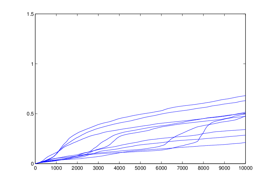
Due to poor regularity properties, we do not expect the numerical approximation to be very accurate, but still we first tried a relatively poor discretization with $N=128$ Fourier-modes and time-steps $h=10^{-4}$ with a terminal time $T=1$ . As expected this did not work that well, and the error is only a little bit smaller than the solution, see Figure 4. Thus we used in our example

N=256\quad\text{and}\quad h=10^{-6}\;.

To simplify the example a little bit, we consider the initial condition $u_{0}=u_{\star}=\sin(x)$ so that the projection to the high modes $Q_{N}u_{\star}=0$ vanishes, and we can neglect all error terms arising from the initial condition.

First in Figure 1 we plotted the residual $\mathcal{K}_{m}^{4}$ for $m=1,\cdots,1/h$ together with the final error. As expected $\mathcal{K}_{m}^{4}$ is small and the error term from Theorem 13 is bounded by the error term involving $\mathcal{K}_{m}^{2}$ and the numerical data.

In Figure 2 we plot two terms of the residual $\mathcal{K}_{m}^{4}$ , for $m=1,\cdots,1/h$ . One of the main terms in $\mathcal{K}_{m}^{4}$ which depends on the numerical data is $\text{Res}_{n}^{dat}$ , therefore we plot $h\sum_{n=1}^{m}\|\text{Res}_{n}^{dat}\|_{L_{4}}^{4}$ in Figure 2(b) to see impact of these terms on the residual-bound $\mathcal{K}_{m}^{4}$ , which seems to be negligible.

Refer to caption — (a) $\mathcal{K}_{m}^{4}$

Moreover in Figure 2(a) we plot $h\sum_{n=0}^{m}\mathcal{S}_{h}(Z_{n+1}-e^{hA}Z_{n})$ , i.e, the term in $\mathcal{K}_{m}^{4}$ which arises from the OU-bridge. By comparing Figure 1(a) and 2(a) we can see the impact of the OU-bridge on $\mathcal{K}_{m}^{4}$ . This gives a substantial, but not the most dominant term in $\mathcal{K}_{m}^{4}$ . We can also see that this error term is almost growing linear. The reason for this is that the part in $\mathcal{S}_{h}$ that depends on the numerical data $Z_{n}$ is quite small and the deterministic part of the estimate dominates, which bounds the fluctuations of the OU-bridge between the data points.

The final bound for the error $\mathbb{E}\left[\|r(mh)\|^{2}_{L_{2}}|(Z_{k})_{k\in\mathbb{N}}\right]$ which is stated in Theorem 13 is plotted in Figure 3 for $10$ simulations. It confirms that the numerical approximation with $N=256$ and $h=10^{-6}$ works well, in contrast to the case $N=128$ and $h=10^{-4}$ . See Figure 4.

We also see in Figure 3 and even better in Figure 4 that the error is not growing with constant speed, but it has parts where it grows much faster. This effect is also very well visible in Figure 2(b), although the effect there is too small to have an impact on $\mathcal{K}_{m}$ . We conjecture that this might be a large deviation effect, that actually might not be that rare due to noise strength of order one.

Let us also point out that we do not expect to have a mean-square error bound without conditioning on the numerical data. Thus both in Figure 3 and 4 we expected a quite large variation for different realizations of the numerical approximation.

To see exactly the impact of each term in $\mathcal{K}_{m}$ we plotted its value in Figure 5. Also in Table 1 values of each term at the final time $T=1$ is stated for $4$ simulations.

$\mathcal{K}_{m}$	$0.1027$	$0.0996$	$0.1055$	$0.1085$
$E_{1}$	$0.0030$	$0.0012$	$0.0038$	$0.0076$
$E_{2}$	$0.0367$	$0.0367$	$0.0367$	$0.0367$
$E_{3}$	$0.0014$	$0.00141$	$0.0014$	$0.00141$
$E_{4}$	$0.0233$	$0.0220$	$0.0253$	$0.0246$
$E_{5}$	$0.03831$	$0.0383$	$0.03830$	$0.0383$

Table 1: Values of four simulations of

\mathcal{K}_{m}

and each of it’s term at the final time

T=1

, i.e,

m=10^{6}

. The contribution of error at discretization points is

E_{1}=\Big(h\sum_{n=1}^{m}\|\text{Res}^{\text{dat}}_{n}\|_{L_{4}}^{4}\Big)^{1/4}

for the part determined by the data and

E_{2}=\Big(\frac{3mh}{8\pi}\Big)^{1/4}\Big(\sum_{k>N}\frac{\alpha_{k}^{2}}{k^{2}}\Big)^{1/2}

for the stochastics on the high modes. The next two error terms

E_{3}=\Big(\frac{h^{5}}{5}\sum_{n=0}^{m}\|Au_{n}\|_{L^{4}}^{4}ds\Big)^{1/4}

and

E_{4}=\Big(h^{2}\sum_{n=0}^{m}\Big[\frac{1}{2}\|u_{n}\|_{L^{12}}^{3}+\cdots+\frac{1}{20}\|d_{n+1}\|_{L^{12}}^{3}\Big]\Big)^{1/4}

are data controlled terms for error that arises between discretization points. Finally

E_{5}=\Big(h\sum_{n=0}^{m}\mathcal{S}_{h}(Z_{n+1}-e^{hA}Z_{n})\Big)^{1/4}

bounding the stochastic fluctuation in between discretization points is large, but not that large as we would expected it to be.

References

[1] A. Alabert, I. Gyöngy, On numerical approximation of stochastic Burgers equation, From stochastic calculus to mathematical finance, Springer, Berlin, 2006, 1–15.
[2] S. Bartels, A posteriori error analysis for time-dependent Ginzburg-Landau type equations, Numer. Math. 99 (2005), no. 4, 557-583.
[3] S. Bartels, R. Müller, O. Christoph, Robust a priori and a posteriori error analysis for the approximation of Allen-Cahn and Ginzburg-Landau equations past topological changes, SIAM J. Numer. Anal. 49 (2011), no. 1, 110-134.
[4] S. Becker, A. Jentzen, Strong convergence rates for nonlinearity-truncated Euler-type approximations of stochastic Ginzburg-Landau equations. ArXiv (2016).
[5] D. Blömker, A. Jentzen, Galerkin Approximations for the Stochastic Burgers Equation, SIAM J. Numer. Anal. 51-1 (2013), 694-715.
[6] D. Blömker, C. Nolde, J.C. Robinson, Rigorous Numerical Verification of Uniqueness and Smoothness in a Surface Growth Model, Journal of Mathematical Analysis and Applications 429(1):311–325, 2015.
[7] D. Blömker, M. Romito, Stochastic PDEs and lack of regularity (A surface growth equation with noise: existence, uniqueness, and blow-up) Jahresbericht der Deutschen Mathematiker-Vereinigung, 117(4):233-286, 2015.
[8] T. Butler, C. Dawson, T. Wildey, A posteriori error analysis of stochastic differential equations using polynomial chaos expansions, SIAM J. Sci. Comput. 33 (2011), no. 3, 1267–1291.
[9] G. Da Prato, J. Zabczyk, Stochastic equations in infinite dimensions. 2nd ed., vol. 152 of Encyclopedia of of Mathematics and its Applications. Cambridge University Press, Cambridge, (2014).
[10] E.H. Georgoulis, C. Makridakis, On a posteriori error control for the Allen-Cahn problem, Math. Methods Appl. Sci. 37 (2014), no. 2, 173–179.
[11] B. Goldys, B. Maslowski, The Ornstein–Uhlenbeck bridge and applications to Markov semigroups Stoch. Proc. Appl. (2008) 18(10), 1738-1767.
[12] M. Hutzenthaler and A. Jentzen, Numerical approximations of stochastic differential equations with non-globally Lipschitz continuous coefficients, vol. 236, American Mathematical Society, 2015.
[13] M. Hutzenthaler, A. Jentzen, and P. E. Kloeden, Strong and weak divergence in finite time of euler’s method for stochastic differential equations with non-globally lipschitz continuous coefficients, in Proceedings of the Royal Society of London A: Mathematical, Physical and Engineering Sciences, vol. 467, The Royal Society, 2011, pp. 1563–1576.
[14] A. Jentzen, P. Kloeden, G. Winkel, Efficient simulation of nonlinear parabolic Spdes with additive noise, Annals of Applied Probability. 21(3) (2011), 908–950.
[15] E.A. Kalpinelli, N.E. Frangos, A.N. Yannacopoulos, Numerical methods for hyperbolic SPDEs: a Wiener chaos approach, Stoch. Partial Differ. Equ. Anal. Comput. 1 (2013), no. 4, 606–633.
[16] P.E. Kloeden, G.J. Lord, A. Neuenkirch, T. Shardlow, The exponential integrator scheme for stochastic partial differential equations: Pathwise error bounds. J. Comput. Appl. Math. 235, No. 5, 1245.–1260 (2011).
[17] G.J. Lord, C.E. Powell, T. Shardlow, An introduction to computational stochastic PDEs. Cambridge Texts in Applied Mathematics. Cambridge: Cambridge University Press, (2014).
[18] C. Nolde, Global regularity and uniqueness of solutions in a surface growth model using rigorous a-posteriori methods. PhD-thesis, Universit’́at Augsburg, 2017.
[19] K.-Y. Moon, E. von Schwerin, A. Szepessy, R. Tempone, An adaptive algorithm for ordinary, stochastic and partial differential equations. Recent advances in adaptive computation, 325–343, Contemp. Math., 383, Amer. Math. Soc., Providence, RI, 2005
[20] R. Verfürth, A posteriori error estimation techniques for finite element methods, in “Numerical Mathematics and Scientific Computation.” Oxford University Press, Oxford, 2013.
[21] X. Yang, Y. Duan, Y. Guo, A posteriori error estimates for finite element approximation of unsteady incompressible stochastic Navier-Stokes equations, SIAM J. Numer. Anal. 48 (2010), no. 4, 1579–1600.
[22] X. Yang, R. Qi, Y. Duan, A posteriori analysis of finite element discretizations of stochastic partial differential delay equations. J. Difference Equ. Appl. 18 (2012), no. 10, 1649–1663.