An Algorithm for Computing the Distribution Function of the Generalized Poisson-Binomial Distribution

Because each indicator $I_{k}$ can take values in $\{0,1\}$, all possible combinations can be denoted by

$\displaystyle\mathbf{B}=\underbrace{\{0,1\}\times\cdots\times\{0,1\}\times\cdots\times\{0,1\}}_{n\textrm{ times}}.$

Let $\boldsymbol{r}=(r_{1},\cdots,r_{k},\cdots,r_{n})^{\prime}$ be an element in $\mathbf{B}$. The number of elements in $\mathbf{B}$ is $2^{n}$. The value of each element of $\boldsymbol{r}$ is either 0 or 1. The set of all possible values of $X$ is

$\displaystyle\mathbf{X}=\left\{x:\textrm{ there exists at least one }\boldsymbol{r}\textrm{ such that }x=\sum_{k=1}^{n}a_{k}r_{k}+b_{k}r_{k}\right\}.$

Let $a=\sum_{k=1}^{n}a_{k}$ and $b=\sum_{k=1}^{n}b_{k}$. The possible values for $X$ ranges from $a$ to $b$, and evidently

$\displaystyle\Pr(X=x)=\sum_{\boldsymbol{r}\in\mathbf{S}_{x}}\prod_{k=1}^{n}p_{k}^{r_{k}}(1-p_{k})^{1-r_{k}},$

where $\mathbf{S}_{x}=\{\boldsymbol{r}:x=\sum_{k=1}^{n}a_{k}r_{k}+b_{k}r_{k}\}$.

An alternative way of calculating the pmf is based on permutation. Let $\{k_{1},k_{2},\cdots,k_{n}\}$ be a permutation of indices $\{1,2,\cdots,n\}$. A possible value of $X$ is $x=\sum_{l=1}^{R}a_{k_{l}}+\sum_{l=R+1}^{n}b_{k_{l}}$, for $R=0,1,\dotsc n$. It is evident that $X=\sum_{l=1}^{R}a_{k_{l}}+\sum_{l=R+1}^{n}b_{k_{l}}$ if and only if $I_{k_{1}}=I_{k_{2}}=\cdots=I_{k_{R}}=0$ and all other $I_{i}$’s are 1. The corresponding probability is

$$\Pr(I_{k_{1}}=I_{k_{2}}=\cdots=I_{k_{R}}=0,\textrm{ all other }I_{i}\textrm{'s}=1)=\left[\prod_{l=1}^{R}(1-p_{k_{l}})\right]\times\left[\prod_{l=R+1}^{n}p_{k_{l}}\right].$$

Thus,

$$\Pr\left(X=\sum_{l=1}^{R}a_{k_{l}}+\sum_{l=R+1}^{n}b_{k_{l}}\right)=\frac{1}{R!(n-R)!}\sum_{S}\left[\prod_{l=1}^{R}(1-p_{k_{l}})\right]\times\left[\prod_{l=R+1}^{n}p_{k_{l}}\right],$$

where $S$ is the sum over all $n!$ permutations of $\{1,2,\cdots,n\}$. The pmf of $X$ can be obtained by aggregating those probabilities for those with the same $x$ values.

Note that both the enumeration and permutation based methods can be computationally infeasible for large $n$ (e.g., when $n>30$). When $n=30$, $2^{30}$ is around 1 billion, and $30!$ is around $2.6\times 10^{32}$. Thus, a computationally efficient method needs to be developed, which will be presented in next section.

For the development of the algorithm, we restrict $a_{k}$ and $b_{k}$ to be integers. We will discuss non-integer cases later in Section 4. Let

$$\xi_{j}=\Pr(X=j+a),j=0,\cdots,m,$$

be the probability mass function (pmf) of $X$, where $a=\sum_{k=1}^{n}a_{k}$, $b=\sum_{k=1}^{n}b_{k}$, and $m=b-a$. The objective is to compute the pmf $\{\xi_{0},\xi_{1},\cdots,\xi_{m}\}$. The characteristic function (cf) of $X$ is

$\displaystyle\varphi(t)=\mathbf{E}[\exp({\boldsymbol{i}}tX)]=\sum_{j=0}^{m}\xi_{j}\exp[{\boldsymbol{i}}t(j+a)],$

(2)

where ${\boldsymbol{i}}=\sqrt{-1}$. Alternatively, the cf can be computed as

	$\displaystyle\varphi(t)$	$\displaystyle=\mathbf{E}\left\{\exp\left[{\boldsymbol{i}}t\sum_{k=1}^{n}a_{k}(1-I_{k})+b_{k}I_{k}\right]\right\}$		(3)
		$\displaystyle=\prod_{k=1}^{n}\left[(1-p_{k})\exp({\boldsymbol{i}}ta_{k})+p_{k}\exp({\boldsymbol{i}}tb_{k})\right].$

Linking (2) and (3), we obtain,

$\displaystyle\sum_{j=0}^{m}\xi_{j}\exp({\boldsymbol{i}}tj)=\exp[-{\boldsymbol{i}}ta]\prod_{k=1}^{n}\left[(1-p_{k})\exp({\boldsymbol{i}}ta_{k})+p_{k}\exp({\boldsymbol{i}}tb_{k})\right].$

(4)

Let $\omega=2\pi/(m+1)$. By substituting $t=\omega l,l=0,1,\cdots,m$ into (4), we obtain

	$\displaystyle\frac{1}{m+1}\sum_{j=0}^{m}\xi_{j}\exp({\boldsymbol{i}}\omega lj)$	$\displaystyle=\frac{1}{m+1}\exp[-{\boldsymbol{i}}\omega la]\prod_{k=1}^{n}\left[(1-p_{k})\exp({\boldsymbol{i}}\omega la_{k})+p_{k}\exp({\boldsymbol{i}}\omega lb_{k})\right]$		(5)
		$\displaystyle=\frac{1}{m+1}x_{l},\quad l=0,1,\cdots,m.$

Here,

$$x_{l}=\exp[-{\boldsymbol{i}}\omega la]\prod_{k=1}^{n}\left[(1-p_{k})\exp({\boldsymbol{i}}\omega la_{k})+p_{k}\exp({\boldsymbol{i}}\omega lb_{k})\right].$$

The left hand side of (5) is exactly the inverse discrete Fourier transform (IDFT) of $\{\xi_{0},\xi_{1},$ $\cdots,\xi_{m}\}$ (e.g., see [Bracewell 2000]). Thus, we can recover $\{\xi_{0},\xi_{1},\cdots,\xi_{m}\}$ by applying the discrete Fourier transform (DFT) to both sides of (5). That is,

$\displaystyle\xi_{j}$

$\displaystyle=\frac{1}{m+1}\sum_{l=0}^{m}\exp(-{\boldsymbol{i}}\omega lk)x_{l}.$

One first needs to compute $x_{l}$ and then one can obtain $\xi_{j},j=0,1,\dots,m$. Note that $x_{l}$ can be represented as $x_{l}=u_{l}+{\boldsymbol{i}}v_{l},l=0,1,\dots,m$, where $u_{l}$ and $v_{l}$ are the real and imaginary parts of $x_{l}$, respectively. According to (5),

$$x_{l}=\sum_{j=0}^{m}\xi_{j}\exp({\boldsymbol{i}}\omega lj),l=0,1,\cdots,m.$$

It is evident that $x_{0}=\sum_{k=0}^{n}\xi_{k}=1$. In addition, note that all $\xi_{j}$’s are real numbers and $\exp[{\boldsymbol{i}}\omega(m+1)j]=1$. Thus, the conjugate of $x_{l}$ is

	$\displaystyle\overline{x_{l}}$	$\displaystyle=u_{l}-{\boldsymbol{i}}v_{l}=\sum_{j=0}^{m}\xi_{j}\exp(-{\boldsymbol{i}}\omega lj)=\sum_{j=0}^{m}\xi_{j}\exp[{\boldsymbol{i}}\omega(m+1-l)j]$
		$\displaystyle=x_{m+1-l}=u_{m+1-l}+{\boldsymbol{i}}v_{m+1-l},\quad l=1,\dots,m.$

We obtain $u_{l}=u_{m+1-l}$, and $v_{l}=-v_{m+1-l}$ for $l=1,\dots,m$. Let $z_{0l}=\cos(-\omega la)+{\boldsymbol{i}}\sin(-\omega la),$ and

$$z_{kl}=[(1-p_{k})\cos(\omega la_{k})+p_{k}\cos(\omega lb_{k})]+{\boldsymbol{i}}[(1-p_{k})\sin(\omega la_{k})+p_{k}\sin(\omega lb_{k})].$$

We denote $|z_{kl}|$ as the modulus of $z_{kl}$, and ${\rm Arg}(z_{kl})$ as the principal value of the argument of $z_{kl}$. We obtain

	$\displaystyle x_{l}$	$\displaystyle=\exp\left[\sum_{k=0}^{n}\log(z_{kl})\right]=\exp\left(\sum_{k=0}^{n}\log\left\{|z_{kl}|\exp[{\boldsymbol{i}}{\rm Arg}(z_{kl})]\right\}\right)$
		$\displaystyle=\exp\left[\sum_{k=0}^{n}\log\left(\,|z_{kl}|\,\right)\right]\exp\left[{\boldsymbol{i}}\sum_{k=0}^{n}{\rm Arg}(z_{kl})\right]$
		$\displaystyle=\exp\left[\sum_{k=0}^{n}\log\left(\,|z_{kl}|\,\right)\right]\left\{\cos\left[\sum_{k=0}^{n}{\rm Arg}(z_{kl})\right]+{\boldsymbol{i}}\sin\left[\sum_{k=0}^{n}{\rm Arg}(z_{kl})\right]\right\}.$

In this case, $|z_{0l}|=1$, ${\rm Arg}[z_{0l}]={\rm atan2}\left\{\sin(-\omega la),\cos(-\omega la)\right\}$, and

	$\displaystyle|z_{kl}|$	$\displaystyle=\big\{[(1-p_{k})\cos(\omega la_{k})+p_{k}\cos(\omega lb_{k})]^{2}+[(1-p_{k})\sin(\omega la_{k})+p_{k}\sin(\omega lb_{k})]^{2}\big\}^{\frac{1}{2}},$
	$\displaystyle{\rm Arg}[z_{kl}]$	$\displaystyle={\rm atan2}\left\{[(1-p_{k})\sin(\omega la_{k})+p_{k}\sin(\omega lb_{k})],[(1-p_{k})\cos(\omega la_{k})+p_{k}\cos(\omega lb_{k})]\right\},$

where ${\rm atan2}(y,x)$ is defined as

$${\rm atan2}(y,x)=\begin{cases}\arctan(\frac{y}{x})&\qquad x>0\\ \pi+\arctan(\frac{y}{x})&\qquad y\geq 0,x<0\\ -\pi+\arctan(\frac{y}{x})&\qquad y<0,x<0\\ \frac{\pi}{2}&\qquad y>0,x=0\\ -\frac{\pi}{2}&\qquad y<0,x=0\\ 0&\qquad y=0,x=0\end{cases}.$$

We obtain explicit expressions for $u_{l}$ and $v_{l}$ as

$\displaystyle u_{l}=z_{l}\cos\left[\sum_{k=0}^{n}{\rm Arg}(z_{kl})\right]\text{ and }v_{l}=z_{l}\sin\left[\sum_{k=0}^{n}{\rm Arg}(z_{kl})\right],$

(6)

where $z_{l}=\exp\left[\sum_{k=0}^{n}\log\left(\,|z_{kl}|\,\right)\right],l=1,\dots,m.$

The following algorithm is used to compute the pmf $\xi_{j}$, for $j=0,1,\cdots,m.$
The DFT-CF Algorithm:

1. 1.

   We first assign $x_{0}=1$. Then, we compute the real and imaginary parts of $x_{l}$ by using the formulae in (6), $l=1,\dots[m/2]$, and $[\,\cdot\,]$ is the ceiling function;

2. 2.

   We compute the real and imaginary parts of $x_{l}$ by using the formula $u_{l}=u_{m+1-l}$, and $v_{l}=-v_{m+1-l}$, $l=[m/2]+1,\dots,m$.

3. 3.

   We then apply the fast Fourier transform (FFT) algorithm to the set $\{x_{0}/(m+1),x_{1}/(m+1),\dots,x_{n}/(m+1)\}$ to obtain $\{\xi_{0},\xi_{1},\dots,\xi_{m}\}$.

The DFT-CF algorithm has been implemented in C and it can be called from R. We also wrap the major functions into an R package GPB ([Hong and Zhang 2016]). The use of the R package will be illustrated in Section 4.

We develop an enumeration-based algorithm to compute the exact cdf of the GPB distribution based on theoretical formula. Then, we use the maximum absolute error (MAE) and the total absolute error (TAE) as accuracy metrics by comparing cdf calculated with the DFT-CF algorithm and the enumeration-based method for different values of $n,a_{k},b_{k}$ and $p_{k}$. The maximum absolute error (MAE) is defined as

$${\rm MAE}=\max_{x}|F(x)-F_{{\rm enum}}(x)|,$$

while the total absolute error (TAE) is defined as

$${\rm TAE}=\sum_{x=a}^{b}|F(x)-F_{{\rm enum}}(x)|,$$

where $F(x)$ is the cdf computed by using the DFT-CF algorithm and $F_{{\rm enum}}(x)$ is the cdf computed by using the enumeration formula in Section 2.1.

The accuracy test results are shown in Table 1 for different parameter settings for $n,a_{k},b_{k}$ and $p$. All computations were done on Linux 64-bit server with Intel Xeon CPU (E5-2680, 2.50GHz) and 263 GB RAM. Due to the complex enumeration calculation, the exact method can only handle less than 30 random indicators (i.e., $n=30$) under the capacity of the computer server. Table 3 shows the accuracy of the cdf calculated with the DFT-CF algorithm for various values of $n,a_{k},b_{k}$ and $p$. The MAE are generally less than $5\times 10^{-15}$ and the TAE are less than $5\times 10^{-14}$ for the DFT-CF algorithm, when $n$ is less than 20. Overall, the results show that the DFT-CF algorithm can accurately compute the cdf of the GPB distribution.

To test the accuracy of the DFT-CF algorithm for large values of $m$ and $n$, we compare the cdf computed by the DFT-CF algorithm with that of binomial distributions. As mentioned earlier, the binomial distribution is a special case of the GPB distribution when all $p_{k}$’s are the same, and $a_{k}=0,b_{k}=1$ for all $n$ random indicators. Thus in this comparison setting, we let $p_{k}=p$ to be the same, and $a_{k}=0,b_{k}=1$. That is,

$$X=\sum_{k=1}^{n}a_{k}(1-I_{k})+b_{k}I_{k}=\sum_{k=1}^{n}I_{k}.$$

The exact pmf of X can be calculated from the binomial distribution as

$$\Pr(X=x)={{n}\choose{x}}p^{x}(1-p)^{n-x}.$$

Here again, the MAE and TAE are used as accuracy metrics, which are given by

$${\rm MAE}=\max_{x}|F(k)-F_{{\rm bin}}(k)|,\quad\textrm{ and }\quad{\rm TAE}=\sum_{x=0}^{n}|F(x)-F_{{\rm bin}}(x)|,$$

where $F(x)$ is the cdf computed by the DFT-CF algorithm and $F_{{\rm bin}}(x)$ is the cdf computed using the binomial distribution function implemented in R (?). The accuracy test results are shown in Table 2 with different parameter settings for $n,a_{k},b_{k}$ and $p$. Basically, the TAE and MAE accumulate as $n,p$ and $a_{k},b_{k}$ increases. When $n$ is less than 10,000, the MAE is within $1\times 10^{-12}$ and TAE is under $1\times 10^{-8}$. The results in Table 2 show that the DFT-CF algorithm can accurately compute the cdf for large $n$. With no available efficient algorithm developed for computing the GPB distribution, the proposed method provides an important alternative to model real-life applications.

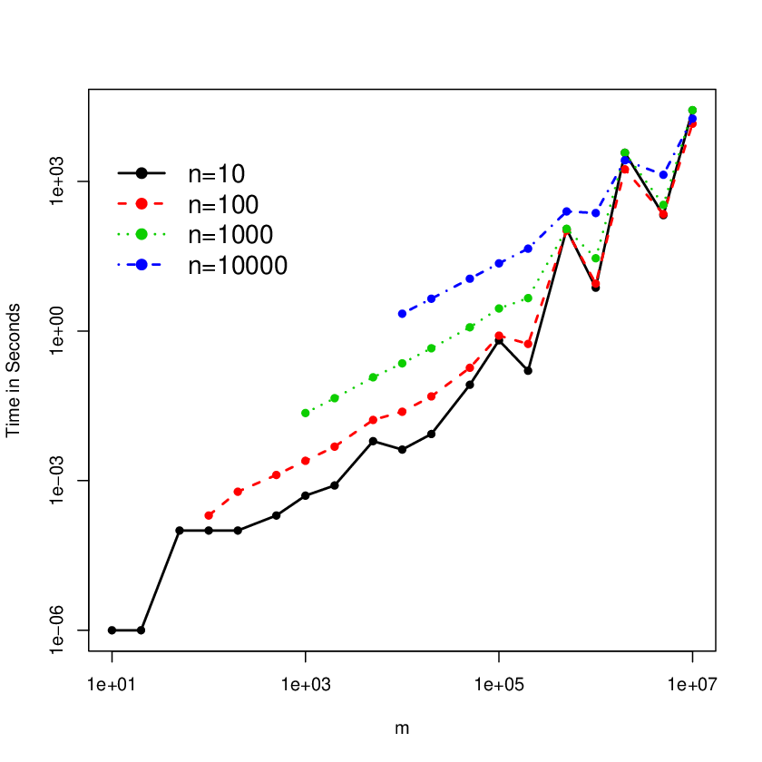
The computational time of the DFT-CF algorithm is mostly determined by $n$ and $m$. Note that $m=b-a=\sum_{k=1}^{n}b_{k}-\sum_{k=1}^{n}a_{k}$. We first consider the computational time when $n$ is large. We first choose 10 $p$’s from [0.01, 0.99], and for different values of $n$ and $m$, we set $p_{k}=p,a_{k}=0,b_{k}=1$ for all $n$ indicators. The time for calculating the entire cdf using the DFT-CF algorithm is averaged across 10 $p$’s, which are shown in Table 3. The unit of computation time is second.

Figure 1 visualizes the results in Table 3. Both the x-axis and y-axis are on log scales. Each line indicates the average computation time for a specific $n$, where $n=10$, 100, 1,000, and 10,000. Figure 1 shows that as $n$ increases, the computational time increases exponentially. The computational time is negligible (less than 10 milliseconds) when $n\leq 100$. When $n$ is fixed at 10, 100, 1,000, and 10,000, the general average computational time increases as $m$ increases. However, there are minor drops in computational time even when $m$ increases to big numbers. The DFT-CF algorithm can work out $n\leq 10{,}000$ and $m\leq 1{,}000{,}000$ within 5 minutes. As $n$ exceeds 10,000 and $m$ exceeds 1,000,000, the DFT-CF algorithm requires more than 5 minutes. Overall, the DFT-CF algorithm shows reasonable computational efficiency.

The DFT-CF algorithm has been implemented in the R package GPB, ?), which can be downloaded from the Comprehensive R Archive Network (http://cran.r-project.org/). The R functions for computing the cdf, pmf, quantile function and random number generation are all available in the R package. For example, the function pgpb() takes $p_{k}$’s, $a_{k}$’s and $b_{k}$’s as input and computes the cdf of the distribution. See the following R code for reference.

library(GPB)
pgpb(kk=6:9,pp=c(0.1,0.2,0.3),aval=c(1,2,3),bval=c(2,3,4),
wts=c(1,1,1))

Here, kk is $x$ (i.e., the values where the cdf to be evaluated), pp is the vector of $p_{k}$’s, aval is the vector of $a_{k}$’s, bval is the vector of $b_{k}$’s, and wts is the vector of weights for $p_{k}$’s.

There are a few tips in the use of the algorithm. One can use the weights option to speed up the computing when the $p_{k}$’s are the same. For example, if there are 1,000 random indicators with same $p$, instead of replicating the same random indicator 1,000 times, one can specify wts=1,000. The use of wts argument will speed up the computing due to the implementation of the algorithm.

The proposed algorithm can be slow in cases where $n$ and $m$ are extremely large. In some cases, the problem can be eased by taking out the greatest common divider of $a_{k}$’s and $b_{k}$’s. For example, when $k=1,2,\dots,10$, $a_{k}={10,20,\dots,100}$, and $b_{k}={100,200,\dots,1{,}000}$, the cdf is equivalent to the cdf when $a_{k}={1,2,\dots,10}$ and $b_{k}={10,20,\dots,100}$, with a multiplier of 10 for the support values. Thus, by taking out the great common divider, we can shorten the computational time especially when $m$ is large and the common dividers between $a_{k}$’s and $b_{k}$’s are large. See the following R code for reference.

pgpb(kk=seq(10,100,by=10), pp=c(.1, .2, .3), aval=c(10,20,30),
bval=c(20,30,40), wts=c(1,1,1))
pgpb(kk=1:10, pp=c(.1, .2, .3), aval=c(1,2,3), bval=c(2,3,4),
wts=c(1,1,1))

Though the algorithm is derived based on $a_{k}$ and $b_{k}$ being integers, it can be applied to non-integer cases by multiplying powers of $10$ to convert decimal digits into integers. For example, if $a_{k}=\{0.5,1.5,\dots,9.5\}$, $b_{k}=\{1,2,\dots,10\}$, and cdf needs to be computed at $x=50.5$, then we can multiply the set of $a_{k}$, $b_{k}$ and $x$ by 10. The cdf value is the same as being computed at $x=505$ with $a_{k}=\{5,15,\dots,95\}$ and $b_{k}=\{10,20,\dots,100\}$. Note that the multiplication by powers of 10 increases $m$ and correspondingly increases the computation time. However, this process can extend the proposed algorithm to the cases of non-integer numbers. See the following R code for reference.

aval=seq(0.5,9.5,by=1)*10
bval=seq(1,10,by=1)*10
pgpb(kk=50.5*10,pp=seq(0.1,0.5,length.out=10),aval=aval,
bval=bval,wts=rep(1,10))

References

- Alger 2006 Alger, D. (2006). Voting by proxy. Public Choice 126(1), 1–26.
- Bossavy, Girard, and Kariniotakis 2013 Bossavy, A., R. Girard, and G. Kariniotakis (2013). Forecasting ramps of wind power production with numerical weather prediction ensembles. Wind Energy 16, 51–63.
- Bracewell 2000 Bracewell, R. (2000). The Fourier Transform & Its Applications (Third ed.). Singapore: McGraw-Hill, Inc.
- Chen and Liu 1997 Chen, S. X. and J. S. Liu (1997). Statistical applications of the Poisson-binomial and conditional Bernoulli distributions. Statistica Sinica 7, 875–892.
- Cheng and Duncan 2014 Cheng, M. C. N. and J. F. R. Duncan (2014). Rademacher Sums and Rademacher Series, pp. 143–182. Berlin, Heidelberg: Springer.
- Dilworth and Montgomery-Smith 1993 Dilworth, S. J. and S. J. Montgomery-Smith (1993). The distribution of vector-valued Radmacher series. Annals of Probability 21, 2046–2052.
- Duffie, Saita, and Wang 2007 Duffie, D., L. Saita, and K. Wang (2007). Multi-period corporate default prediction with stochastic covariates. Journal of Financial Economics 83, 635–665.
- Hong 2013 Hong, Y. (2013). On computing the distribution function for the Poisson bionomial distribution. Computational Statistics and Data Analysis 59, 41–51.
- Hong and Meeker 2013 Hong, Y. and W. Q. Meeker (2013). Field-failure predictions based on failure-time data with dynamic covariate information. Technometrics 55, 135–149.
- Hong and Zhang 2016 Hong, Y. and M. Zhang (2016). GPB: Generalized Poisson Binomial Distribution. R package version 1.0.
- Montgomery-Smith 1990 Montgomery-Smith, S. J. (1990). The distribution of rademacher sums. Proceedings of the American Mathematical Society 109, 517.
- Niida, Imoto, Shimamura, and Miyano 2012 Niida, A., S. Imoto, T. Shimamura, and S. Miyano (2012). Statistical model-based testing to evaluate the recurrence of genomic aberrations. Bioinformatics 28, i115–i120.
- Pitacco 2007
Pitacco, E. (2007).
Mortality and longevity: A risk management perspective.
In IAA Life Colloquium, Stockholm, available at
http://www.actuaries.org/LIFE/Events/Stockholm/Pitacco.pdf. - R Development Core Team 2016 R Development Core Team (2016). R: A Language and Environment for Statistical Computing. Vienna, Austria: R Foundation for Statistical Computing.
- Tang and Peterson 2011 Tang, P. and E. A. Peterson (2011). Mining probabilistic frequent closed itemsets in uncertain databases. In Proceedings of the 49th ACM Southeast Conference (ACMSE), Kennesaw, GA, pp. 86–91.