跳到论文正文
W Papers独立论文阅读器 arXiv:1702.01286 论文正文 计算阅读时间 · 0%
引用这篇论文根据当前论文元数据生成,正式投稿前建议核对。


License: arXiv.org perpetual non-exclusive license
arXiv:1702.01286v2 [cs.DS] 11 Apr 2017

An Adaptive Sublinear-Time Block Sparse Fourier Transform

Volkan Cevher Affiliation: EPFL    Michael Kapralov Affiliation: EPFL    Jonathan Scarlett Affiliation: EPFL    Amir Zandieh Affiliation: EPFL
Abstract

The problem of approximately computing the kk dominant Fourier coefficients of a vector XX quickly, and using few samples in time domain, is known as the Sparse Fourier Transform (sparse FFT) problem. A long line of work on the sparse FFT has resulted in algorithms with O⁡(k​log⁡n​log⁡(n/k))O(k\log n\log(n/k)) runtime [Hassanieh et al., STOC’12] and O⁡(k​log⁡n)O(k\log n) sample complexity [Indyk et al., FOCS’14]. These results are proved using non-adaptive algorithms, and the latter O⁡(k​log⁡n)O(k\log n) sample complexity result is essentially the best possible under the sparsity assumption alone: It is known that even adaptive algorithms must use Ω⁡((k​log⁡(n/k))/log⁡log⁡n)\Omega((k\log(n/k))/\log\log n) samples [Hassanieh et al., STOC’12]. By adaptive, we mean being able to exploit previous samples in guiding the selection of further samples.

This paper revisits the sparse FFT problem with the added twist that the sparse coefficients approximately obey a (k0,k1)(k_{0},k_{1})-block sparse model. In this model, signal frequencies are clustered in k0k_{0} intervals with width k1k_{1} in Fourier space, and k=k0​k1k=k_{0}k_{1} is the total sparsity. Signals arising in applications are often well approximated by this model with k0≪kk_{0}\ll k.

Our main result is the first sparse FFT algorithm for (k0,k1)(k_{0},k_{1})-block sparse signals with a sample complexity of O∗​(k0​k1+k0​log⁡(1+k0)​log​n)O^{*}(k_{0}k_{1}+k_{0}\log(1+k_{0})\log n) at constant signal-to-noise ratios, and sublinear runtime. A similar sample complexity was previously achieved in the works on model-based compressive sensing using random Gaussian measurements, but used Ω⁡(n)\Omega(n) runtime. To the best of our knowledge, our result is the first sublinear-time algorithm for model based compressed sensing, and the first sparse FFT result that goes below the O⁡(k​log⁡n)O(k\log n) sample complexity bound.

Interestingly, the aforementioned model-based compressive sensing result that relies on Gaussian measurements is non-adaptive, whereas our algorithm crucially uses adaptivity to achieve the improved sample complexity bound. We prove that adaptivity is in fact necessary in the Fourier setting: Any non-adaptive algorithm must use Ω⁡(k0​k1​log⁡nk0​k1)\Omega(k_{0}k_{1}\log\frac{n}{k_{0}k_{1}}) samples for the (k0,k1CLOSE(k_{0},k_{1})-block sparse model, ruling out improvements over the vanilla sparsity assumption. Our main technical innovation for adaptivity is a new randomized energy-based importance sampling technique that may be of independent interest.

1 Introduction

The discrete Fourier transform (DFT) is one of the most important tools in modern signal processing, finding applications in audio and video compression, radar, geophysics, medical imaging, communications, and many more. The best known algorithm for computing the DFT of a general signal of length nn is the Fast Fourier Transform (FFT), taking O⁡(n​log⁡n)O(n\log n) time, which matches the trivial Ω⁡(n)\Omega(n) lower bound up to a logarithmic factor.

In recent years, significant attention has been paid to exploiting sparsity in the signal’s Fourier spectrum, which is naturally the case for numerous of the above applications. By sparse, we mean that the signal can be well-approximated by a small number of Fourier coefficients. Given this assumption, the computational lower bound of Ω⁡(n)\Omega(n) no longer applies. Indeed, the DFT can be computed in sublinear time, while using a sublinear number of samples in the time domain [GIIS14, GST08].

The problem of computing the DFT of signals that are approximately sparse in the Fourier domain has received significant attention in several communities. The seminal work of [CT06a, RV08] in compressive sensing first showed that only k​logO⁡(1)​nk\log^{O(1)}n samples in time domain suffice to recover a length nn signal with at most kk nonzero Fourier coefficients. A different line of research on the Sparse Fourier Transform (sparse FFT), with origins in computational complexity and learning theory, has resulted in algorithms that use k​logO⁡(1)​nk\log^{O(1)}n samples and k​logO⁡(1)​nk\log^{O(1)}n runtime (i.e., the runtime is sublinear in the length of the input signal). Many such algorithms have been proposed in the literature [GL89, KM91, Man92, GGI+02, AGS03, GMS05, Iwe10, Aka10, HIKP12b, HIKP12a, LWC12, BCG+12, HAKI12, PR13, HKPV13, IKP14, IK14, Kap16, PS15]; we refer the reader to the recent surveys [GIIS14, GST08] for a more complete overview.

The best known runtime for computing the kk-sparse FFT is due to Hassanieh et al. [HIKP12a], and is given by O⁡(k​log⁡n​log⁡(n/k))O(k\log n\log(n/k)), asymptotically improving upon the FFT for all k=o⁡(n)k=o(n). The recent works of [IKP14, Kap16] also show how to achieve a sample complexity of O⁡(k​log⁡n)O(k\log n) (which is essentially optimal) in linear time, or in time k​logO⁡(1)​nk\log^{O(1)}n at the expense of poly⁡(log⁡log⁡n)\mathrm{poly}(\log\log n) factors. Intriguingly, the aforementioned algorithms are all non-adaptive. That is, these algorithms do not exploit existing samples in guiding the selection of the new samples to improve approximation quality. In the same setting, it is also known that adaptivity cannot improve the sample complexity by more than an O⁡(log⁡log⁡n)O(\log\log n) factor [HIKP12a].

Despite the significant gains permitted by sparsity, designing an algorithm for handling arbitrary sparsity patterns may be overly generic; in practice, signals often exhibit more specific sparsity structures. A common example is block sparsity, where significant coefficients tend to cluster on known partitions, as opposed to being unrestricted in the signal spectrum. Other common examples include tree-based sparsity, group sparsity, and dispersive sparsity [BCDH10, BBC+16, EHC15, Bac10].

Such structured sparsity models can be captured via the model-based framework [BCDH10], where the number of sparsity patterns may be far lower than (nk){n\choose k}. For the compressive sensing problem, this restriction has been shown to translate into a reduction in the sample complexity, even with non-adaptive algorithms. Specifically, one can achieve a sample complexity of O⁡(k+log⁡|ℳ|)O(k+\log|\mathcal{M}|) with dense measurement matrices based on the Gaussian distribution, where ℳ\mathcal{M} is the set of permitted sparsity patterns. Reductions in the sample complexity with other types of measurement matrices, e.g., sparse matrices based on expanders, are typically less [BBC14, IR13]. Other benefits of exploiting model-based sparsity include faster recovery and improved noise robustness [BCDH10, BBC14].

Surprisingly, in stark contrast to the extensive work on exploiting model-based sparsity with general linear measurements, there are no existing sparse FFT algorithms exploiting such structure. This paper presents the first such algorithm, focusing on the special case of block sparsity. Even for this relatively simple sparsity model, achieving the desiderata turns out to be quite challenging, needing a whole host of new techniques, and intriguingly, requiring adaptivity in the sampling.

To clarify our contributions, we describe our model and the problem statement in more detail.

Model and Basic Definitions

The Fourier transform of a signal X∈ℂnX\in\mathbb{C}^{n} is denoted by X^\widehat{X}, and defined as

X^f=1n​∑i∈[n]Xi​ωn−f​t,f∈[n],\widehat{X}_{f}=\frac{1}{n}\sum_{i\in[n]}X_{i}\omega_{n}^{-ft},\quad f\in[n],

where ωn\omega_{n} is the nn-th root of unity. With this definition, Parseval’s theorem takes the form ‖X‖2=n​‖X^‖22\|X\|^{2}=n\|\widehat{X}\|_{2}^{2}.

We are interested in computing the Fourier transform of signals that, in frequency domain, are well-approximated by a block sparse signal with k0k_{0} blocks of width k1k_{1}, formalized as follows.

Definition 1.1 (Block sparsity).

Given a sequence X∈ℂnX\in\mathbb{C}^{n} and an even block width k1k_{1}, the jj-th interval is defined as Ij=((j−1/2)​k1,(j+1/2)​k1]∩ℤI_{j}=\big((j-1/2)k_{1},(j+1/2)k_{1}\big]\cap\mathbb{Z} for j∈[nk1]j\in\big[\frac{n}{k_{1}}\big], and we refer to X^Ij\widehat{X}_{I_{j}} as the jj-th block. We say that a signal is (k0,k1)(k_{0},k_{1})-block sparse if it contains non-zero values within at most k0k_{0} of these intervals.

Block sparsity is of direct interest in several applications [BCDH10, BCW10]; we highlight two examples here: (i) In spectrum sensing, cognitive radios seek to improve the utilization efficiency in a sparsely used wideband spectrum. In this setting, the frequency bands being detected are non-overlapping and predefined. (ii) Audio signals often contain blocks corresponding to different sounds at different frequencies. Such blocks may be non-uniform, and can be modeled by the (k,c)(k,c) model in which kk coefficients are arbitrarily spread across cc different clusters. It was argued in [CIHB09] that any signal from the (k,c)(k,c) model is also (3​c,k/c)(3c,k/c)-block sparse in the uniform model.

Our goal is to output a list of frequencies and values estimating X^\widehat{X}, yielding an ℓ2\ell_{2}-distance to X^\widehat{X} not much larger than that of the best (k0,k1)(k_{0},k_{1})-block sparse approximation. Formally, we say that an output signal X^′\widehat{X}^{\prime} satisfies the ℓ2/ℓ2\ell_{2}/\ell_{2} block-sparse recovery guarantee if

‖X^−X^′‖2≤(1+ϵ)​minY^​ is ​(k0,k1)​-block sparse​‖X^−Y^‖2\|\widehat{X}-\widehat{X}^{\prime}\|_{2}\leq(1+\epsilon)\min_{\widehat{Y}\text{ is }(k_{0},k_{1})\text{-block sparse}}\|\widehat{X}-\widehat{Y}\|_{2}

for an input parameter ϵ>0\epsilon>0.

The sample complexity and runtime of our algorithm are parameterized by the signal-to-noise ratio (SNR) of the input signal, defined as follows.

Definition 1.2 (Tail noise and signal-to-noise ratio (SNR)).

We define the tail noise level as

Err⁡(X^,k0,k1)\displaystyle\mathrm{Err}(\widehat{X},k_{0},k_{1}) :=min⁡∑j∈[nk1]\SS⊂[nk1]|S|=k0⁡‖X^Ij‖22,\displaystyle:=\min_{\begin{subarray}{c}S\subset[\frac{n}{k_{1}}]\\ |S|=k_{0}\end{subarray}}\sum_{j\in[\frac{n}{k_{1}}]\backslash S}\|\widehat{X}_{I_{j}}\|_{2}^{2}, (1)

and its normalized version as μ2:=1k0​Err2​(X^,k0,k1)\mu^{2}:=\frac{1}{k_{0}}\mathrm{Err}^{2}(\widehat{X},k_{0},k_{1}), representing the average noise level per block. The signal-to-noise ratio is defined as SNR:=‖X^‖2Err2​(X^,k0,k1)\mathrm{SNR}:=\frac{\|\widehat{X}\|^{2}}{\mathrm{Err}^{2}(\widehat{X},k_{0},k_{1})}.

Throughout the paper, we assume that both nn and k1k_{1} are powers of two. For nn, this is a standard assumption in the sparse FFT literature. As for k1k_{1}, the assumption comes without too much loss of generality, since one can always round the block size up to the nearest power of two and then cover the original k0k_{0} blocks with at most 2​k02k_{0} larger blocks, thus yielding a near-identical recovery problem other than a possible increase in the SNR. We also assume that nk1\frac{n}{k_{1}} exceeds a large absolute constant; if this fails, our stated scaling laws can be obtained using the standard FFT.

We use O∗​(⋅)O^{*}(\cdot) notation to hide log⁡log⁡SNR\log\log\mathrm{SNR}, log⁡log⁡n\log\log n, and log⁡1ϵ\log\frac{1}{\epsilon} factors. Moreover, to simplify the notation in certain lemmas having free parameters that will be set in terms of ϵ\epsilon, we assume throughout the paper that ϵ=Ω⁡(1poly​log⁡n)\epsilon=\Omega\big(\frac{1}{\mathrm{poly}\log n}\big), and hence log⁡1ϵ=O⁡(log⁡log⁡n)\log\frac{1}{\epsilon}=O(\log\log n). This is done purely for convenience, and since the dependence on ϵ\epsilon is not our main focus; the precise expressions with log⁡1ϵ\log\frac{1}{\epsilon} factors are easily inferred from the proofs. Similarly, since the low-SNR regime is not our key focus, we assume that SNR≥2\mathrm{SNR}\geq 2, and thus log⁡SNR\log\mathrm{SNR} is positive.

Contributions.

We proceed by informally stating our main result; a formal statement is given in Section 5.2.

Theorem 1.1.

(Upper bound – informal version) There exists an adaptive algorithm for approximating the Fourier transform with (k0,k1)(k_{0},k_{1})-block sparsity that achieves the ℓ2/ℓ2\ell_{2}/\ell_{2} guarantee for any constant ϵ=Θ⁡(1)\epsilon=\Theta(1), with a sample complexity of O∗​((k0​k1+k0​log⁡(1+k0)​log​n)​log⁡SNR)O^{*}\big((k_{0}k_{1}+k_{0}\log(1+k_{0})\log n)\log\mathrm{SNR}), and a runtime of O∗​((k0​k1​log3​n+k0​log⁡(1+k0)​log2​n)​log​SNR)O^{*}\big((k_{0}k_{1}\log^{3}n+k_{0}\log(1+k_{0})\log^{2}n)\log\mathrm{SNR}).

Note that while we state the result for ϵ=Θ⁡(1)\epsilon=\Theta(1) here, the dependence on this parameter is explicitly shown in the formal version.

The sample complexity of our algorithm strictly improves upon the sample complexity of O⁡(k0​k1​log⁡n)O(k_{0}k_{1}\log n) (essentially optimal under the standard sparsity assumption) when log⁡(1+k0)​log⁡SNR≪k1\log(1+k_{0})\log\mathrm{SNR}\ll k_{1} and log⁡SNR≪log⁡n\log\mathrm{SNR}\ll\log n (e.g., SNR=O⁡(1)\mathrm{SNR}=O(1)).

Our algorithm that achieves the above upper bound crucially uses adaptivity. This is in stark contrast with the standard sparse FFT, where we know how to achieve the near-optimal O⁡(k​log⁡n)O(k\log n) bound using non-adaptive sampling [IKP14]. While relying on adaptivity can be viewed as a weakness, we provide a lower bound revealing that adaptivity is essential for obtaining the above sample complexity gains. We again state an informal version, which is formalized in Section 6.

Theorem 1.2.

(Lower bound – informal version) Any non-adaptive sparse FFT algorithm that achieves the ℓ2/ℓ2\ell_{2}/\ell_{2} sparse recovery guarantee with (k0,k1)(k_{0},k_{1})-block sparsity must use a number of samples behaving as Ω⁡(k0​k1​log⁡nk0​k1)\Omega\big(k_{0}k_{1}\log\frac{n}{k_{0}k_{1}}\big).

To the best of our knowledge, these two theorems provide the first results along several important directions, giving (a) the first sublinear-time algorithm for model-based compressive sensing; (b) the first model-based result with provable sample complexity guarantees in the Fourier setting; (c) the first proven gap between the power of adaptive and non-adaptive sparse FFT algorithms; and (d) the first proven gap between the power of structured (Fourier basis) and unstructured (random Gaussian entries) matrices for model-based compressive sensing.

To see that (d) is true, note that the sample complexity O⁡(k0​log⁡n+k0​k1)O(k_{0}\log n+k_{0}k_{1}) for block-sparse recovery can be achieved non-adaptively using Gaussian measurements [BCDH10], but we show that adaptivity is required in the Fourier setting.

Dependence of our results on SNR. The sample complexity and runtime of our upper bound depend logarithmically on the SNR of the input signal. This dependence is common for sparse FFT algorithms, and even for the case of standard sparsity, algorithms avoiding this dependence in the runtime typically achieve a suboptimal sample complexity [HIKP12b, HIKP12a]. Moreover, to our knowledge, all existing sparse FFT lower bounds consider the constant SNR regime (e.g., [DIPW10, PW11, HIKP12a]).

We also note that our main result, as stated above, assumes that upper bounds on the SNR and the tail noise are known that are tight to within a constant factor (in fact, such tightness is not required, but the resulting bound replaces the true values by the assumed values). These assumptions can be avoided at the expense of a somewhat worse dependence on log⁡SNR\log\mathrm{SNR}, but we prefer to present the algorithm in the above form for clarity. The theoretical guarantees for noise-robust compressive sensing algorithms often require similar assumptions [FR13].

Our techniques:

At a high level, our techniques can be summarized as follows:

Upper bound. The high-level idea of our algorithm is to reduce the (k0,k1)(k_{0},k_{1})-block sparse signal of length nn to a number of downsampled O⁡(k0)O(k_{0})-sparse signals of length nk1\frac{n}{k_{1}}, and use standard sparse FFT techniques to locate their dominant values, thereby identifying the dominant blocks of the original signal. Once the blocks are located, their values can be estimated using hashing techniques. Despite the high-level simplicity, this is a difficult task requiring novel techniques, the most notable of which is an adaptive importance sampling scheme for allocating sparsity budgets to the downsampled signals. Further details are given in Section 2.

Lower bound. Our lower bound for non-adaptive algorithms follows the information-theoretic framework of [PW11], but uses a significantly different ensemble of structured approximately block-sparse signals occupying only a fraction O⁡(1k0​k1)O\big(\frac{1}{k_{0}k_{1}}\big) of the time domain. Hence, whereas the analysis of [PW11] is based on the difficulty of identifying one of (roughly) (nk){n\choose k} sparsity patterns, the difficulty in our setting is in non-adaptively finding where the signal is non-zero – one must take enough samples to cover the various possible time domain locations. The details are given in Section 6.

Interestingly, our upper bound uses adaptivity to circumvent the difficulty exploited in this lower bounding technique, by first determining where the energy lies, and then concentrating the rest of its samples on the “right” parts of the signal.

Notation:

For an even number nn, we define [n]:=(−n2,n2]∩ℤ[n]:=\big(-\frac{n}{2},\frac{n}{2}\big]\cap\mathbb{Z}, where ℤ\mathbb{Z} denotes the integers. When we index signals having a given length mm, all arithmetic should be interpreted as returning values in [m][m] according to modulo-mm arithmetic. For x,y∈ℂx,y\in\mathbb{C} and Δ∈ℝ\Delta\in\mathbb{R}, we write y=x±Δy=x\pm\Delta to mean |y−x|≤Δ|y-x|\leq\Delta. The support of a vector XX is denoted by supp⁡(X)\mathrm{supp}(X). For a number a∈ℝa\in\mathbb{R}, we write |a|+:=max⁡{0,a}|a|_{+}:=\max\{0,a\} to denote the positive part of aa.

Organization:

The paper is organized as follows. In Section 2, we provide an outline of our algorithm and the main challenges involved. We formalize our energy-based importance sampling scheme in Section 3, and provide the corresponding techniques for energy estimation in Section 4. The block-sparse FFT algorithm and its theoretical guarantees are given in Section 5, and the lower bound is presented and proved in Section 6. Several technical proofs are relegated to the appendices.

2 Overview of the Algorithm

One of our key technical contributions consists of a reduction from the (k0,k1)(k_{0},k_{1})-block sparse recovery problem for signals of length nn to O⁡(k0)O(k_{0})-sparse recovery on a set of carefully-defined signals of reduced length n/k1n/k_{1}, in sublinear time. We outline this reduction below.

A basic candidate reduction to O⁡(k0)O(k_{0})-sparse recovery consists of first convolving X^\widehat{X} with a filter G^\widehat{G} whose support approximates the indicator function of the interval [−k1/2,k1/2][-k_{1}/2,k_{1}/2], and then considering a new signal whose Fourier transform consists of samples of X^⋆G^\widehat{X}\star\widehat{G} at multiples of k1k_{1}. The resulting signal Z^\widehat{Z} of length n/k1n/k_{1} (a) naturally represents X^\widehat{X}, as every frequency of this sequence is a (weighted) sum of the frequencies in the corresponding block, and (b) can be accessed in time domain using a small number of accesses to XX (if GG is compactly supported; see below).

This is a natural approach, but its vanilla version does not work: Some blocks in X^\widehat{X} may entirely cancel out, not contributing to Z^\widehat{Z} at all, and other blocks may add up constructively and contribute an overly large amount of energy to Z^\widehat{Z}. To overcome this challenge, we consider not one, but rather 2​k12k_{1} reductions: For each r∈[2​k1]r\in[2k_{1}], we apply the above reduction to the shift of XX by r⋅n2​k1r\cdot\frac{n}{2k_{1}} in time domain, and call the corresponding vector ZrZ^{r}. We show that all shifts cumulatively capture the energy of XX well, and the major contribution of the paper is an algorithm for locating the dominant blocks in X^\widehat{X} from a small number of accesses to the ZrZ^{r}’s (via an importance sampling scheme).

Formal definitions: We formalize the above discussion in the following, starting with the notion of a flat filter that approximates a rectangle.

Definition 2.1 (Flat filter).

A sequence G∈ℝnG\in\mathbb{R}^{n} with Fourier transform G^∈ℝn\widehat{G}\in\mathbb{R}^{n} symmetric about zero is called an (n,B,F)(n,B,F)-flat filter if (i) G^f∈[0,1]\widehat{G}_{f}\in[0,1] for all f∈[n]f\in[n]; (ii) G^f≥1−(14)F−1\widehat{G}_{f}\geq 1-\big(\frac{1}{4}\big)^{F-1} for all f∈[n]f\in[n] such that |f|≤n2​B|f|\leq\frac{n}{2B}; and (iii) G^f≤(14)F−1​(nB​|f|)F−1\widehat{G}_{f}\leq\big(\frac{1}{4}\big)^{F-1}\big(\frac{n}{B|f|}\big)^{F-1} for all f∈[n]f\in[n] such that |f|≥nB|f|\geq\frac{n}{B}.

The following lemma, proved in Appendix A.1, shows that it is possible to construct such a filter having O⁡(F​B)O(FB) support in time domain.

Lemma 2.1.

(Compactly supported flat filter) Fix the integers (n,B,F)(n,B,F) with nn a power of two, B<nB<n, and F≥2F\geq 2 an even number. There exists an (n,B,F)(n,B,F)-flat filter G^∈ℝn\widehat{G}\in\mathbb{R}^{n}, which (i) is supported on a length-O⁡(F​B)O(FB) window centered at zero in time domain, and (ii) has a total energy satisfying ∑f∈[n]|G^f|2≤3​nB\sum_{f\in[n]}|\widehat{G}_{f}|^{2}\leq\frac{3n}{B}.

Throughout the paper, we make use of the filter construction from Lemma 2.1, except where stated otherwise. To ease the analysis, we assume that GG and G^\widehat{G} are pre-computed and can be accessed in O⁡(1)O(1) time. Without this pre-computation, evaluating G^\widehat{G} is non-trivial, but possible using semi-equispaced Fourier transform techniques (cf., Section 4.2).

With the preceding definition, the set of 2​k12k_{1} downsampled signals is given as follows.

Definition 2.2 (Downsampling).

Given integers (n,k1)(n,k_{1}), a parameter δ∈(0,120)\delta\in\big(0,\frac{1}{20}\big), and a signal X∈ℂnX\in\mathbb{C}^{n}, we say that the set of signals {Zr}r∈[2​k1]\{Z^{r}\}_{r\in[2k_{1}]} with Zr∈ℂnk1Z^{r}\in\mathbb{C}^{\frac{n}{k_{1}}} is a (k1,δ)(k_{1},\delta)-downsampling of XX if

Zjr=1k1​∑i∈[k1](G⋅Xr)j+nk1⋅i,j∈[nk1]Z^{r}_{j}=\frac{1}{k_{1}}\sum_{i\in[k_{1}]}(G\cdot X^{r})_{j+\frac{n}{k_{1}}\cdot i},\penalty\ \penalty\ \penalty\ j\in\Big[\frac{n}{k_{1}}\Big]

for an (n,nk1,F)\big(n,\frac{n}{k_{1}},F\big)-flat filter with F=10​log⁡1δF=10\log\frac{1}{\delta} and support O⁡(F​nk1)O\big(F\frac{n}{k_{1}}\big), where we define Xir=Xi+arX^{r}_{i}=X_{i+a_{r}} with ar=n​r2​k1a_{r}=\frac{nr}{2k_{1}}. Equivalently, in frequency domain, this can be written as

Z^jr=(X^r⋆G^)j​k1=∑f∈[n]G^f−k1⋅j​X^f​ωnar⋅f,j∈[nk1]\widehat{Z}^{r}_{j}=(\widehat{X}^{r}\star\widehat{G})_{jk_{1}}=\sum_{f\in[n]}\widehat{G}_{f-k_{1}\cdot j}\widehat{X}_{f}\omega_{n}^{a_{r}\cdot f},\penalty\ \penalty\ \penalty\ j\in\Big[\frac{n}{k_{1}}\Big] (2)

by the convolution theorem and the duality of subsampling and aliasing (e.g., see Appendix C.1).

By the assumption of the bounded support of GG, along with the choice of FF, we immediately obtain the following lemma, showing that we do not significantly increase the sample complexity by working with {Zr}r∈[2​k1]\{Z^{r}\}_{r\in[2k_{1}]} as opposed to XX itself.

Lemma 2.2.

(Sampling the downsampling signals) Let {Zr}r∈[2​k1]\{Z^{r}\}_{r\in[2k_{1}]} be a (k1,δ)(k_{1},\delta)-downsampling of X∈ℂnX\in\mathbb{C}^{n} for some (n,k1,δ)(n,k_{1},\delta). Then any single entry ZirZ_{i}^{r} can be computed in O⁡(log⁡1δ)O\big(\log\frac{1}{\delta}\big) time using O⁡(log⁡1δ)O\big(\log\frac{1}{\delta}\big) samples of XX.

This idea of using 2​k12k_{1} reductions fixes the above-mentioned problem of constructive and destructive cancellations: The 2​k12k_{1} reduced signals ZrZ^{r} (r∈[2​k1]r\in[2k_{1}]) cumulatively capture all the energy of XX well. That is, while the energy |Z^jr|22|\widehat{Z}_{j}^{r}|_{2}^{2} can vary significantly as a function of rr, we can tightly control the behavior of the sum ∑r∈[2​k1]|Z^jr|22\sum_{r\in[2k_{1}]}|\widehat{Z}_{j}^{r}|_{2}^{2}. This is formalized in the following.

Lemma 2.3.

(Downsampling properties) Fix (n,k1)(n,k_{1}), a parameter δ∈(0,120)\delta\in\big(0,\frac{1}{20}\big), a signal X∈ℂnX\in\mathbb{C}^{n}, and a (k1,δ)(k_{1},\delta)-downsampling {Zr}r∈[2​k1]\{Z^{r}\}_{r\in[2k_{1}]} of XX. The following conditions hold:

  1. 1.

    For all j∈[nk1]j\in[\frac{n}{k_{1}}],

    ∑r∈[2​k1]|Z^jr|22​k1≥(1−δ)​‖X^Ij‖22−3​δ⋅(‖X^Ij∪Ij−1∪Ij+1‖22+δ​∑j′∈[nk1]\{j}‖X^Ij′‖22|j′−j|F−1).\frac{\sum_{r\in[2k_{1}]}|\widehat{Z}^{r}_{j}|^{2}}{2k_{1}}\geq(1-\delta)\|\widehat{X}_{I_{j}}\|_{2}^{2}-3\delta\cdot\bigg(\|\widehat{X}_{I_{j}\cup I_{j-1}\cup I_{j+1}}\|_{2}^{2}+\delta\sum_{j^{\prime}\in[\frac{n}{k_{1}}]\backslash\{j\}}\frac{\|\widehat{X}_{I_{j^{\prime}}}\|_{2}^{2}}{|j^{\prime}-j|^{F-1}}\bigg).
  2. 2.

    The total energy satisfies (1−12​δ)​‖X^‖22≤∑r∈[2​k1]‖Z^r‖222​k1≤6​‖X^‖22.(1-12\delta)\|\widehat{X}\|_{2}^{2}\leq\frac{\sum_{r\in[2k_{1}]}\|\widehat{Z}^{r}\|_{2}^{2}}{2k_{1}}\leq 6\|\widehat{X}\|_{2}^{2}.

The proof is given in Appendix A.2.

Location via sparse FFT: We expect each ZrZ^{r} (r∈[2​k1]r\in[2k_{1}]) to be approximately O⁡(k0)O(k_{0})-sparse, as every block contributes primarily to one downsampled coefficient. At this point, a natural step is to run O⁡(k0)O(k_{0})-sparse recovery on the signals ZrZ^{r} to recover the dominant blocks. However, there are too many signals ZrZ^{r} to consider! Indeed, if we were to run O⁡(k0)O(k_{0})-sparse recovery on every ZrZ^{r}, we would recover the locations of the blocks, but at the cost of O⁡(k0​k1​log⁡n)O(k_{0}k_{1}\log n) samples. This precludes any improvement on the vanilla sparse FFT.

It turns out, however, that it is possible to avoid running a k0k_{0}-sparse FFT on all 2​k12k_{1} reduced signals, and to instead allocate budgets to them, some of which are far smaller than k0k_{0}, and some of which may be zero. This will be key in reducing the sample complexity.

Before formally defining budget allocation, we present the following definition and lemma, showing that we can use less samples to identify less of the dominant coefficients of a signal, or more samples to identify more dominant coefficients.

Definition 2.3.

(Covered frequency) Given an integer mm, a frequency component jj of a signal Z^∈ℂm\widehat{Z}\in\mathbb{C}^{m} is called covered by budget ss in the signal Z^\widehat{Z} if |Z^j|2≥‖Z^‖22s|\widehat{Z}_{j}|^{2}\geq\frac{\|\widehat{Z}\|_{2}^{2}}{s}.

Lemma 2.4.

(LocateReducedSignal guarantees – informal version) There exists an algorithm such that if a signal X∈ℂnX\in\mathbb{C}^{n}, a set of budgets {sr}r∈[2​k1]\{s^{r}\}_{r\in[2k_{1}]}, and a confidence parameter pp are given to it as input, then it outputs a list that, with probability at least 1−p1-p, contains any given j∈[nk1]j\in[\frac{n}{k_{1}}] that is covered by srs^{r} in Z^r\widehat{Z}^{r} for some r∈[2​k1]r\in[2k_{1}], where {Z^r}r∈[2​k1]\{\widehat{Z}^{r}\}_{r\in[2k_{1}]} denotes the (k1,δ)(k_{1},\delta)-downsampling of XX. Moreover, the list size is O⁡(∑r∈[2​k1]sr)O\big(\sum_{r\in[2k_{1}]}s^{r}\big), the number of samples that the algorithm takes is O⁡(∑r∈[2​k1]sr​log⁡n)O\big(\sum_{r\in[2k_{1}]}s^{r}\log n\big), and the runtime is O⁡(∑r∈[2​k1]sr​log2​n)O\big(\sum_{r\in[2k_{1}]}s^{r}\log^{2}n\big).11 1 As stated in the formal version, additional terms in the runtime are needed when it comes to subtracting off a current estimate to form a residual signal.

The formal statement and proof are given in Appendix F, and reveal that srs^{r} essentially dictates how many buckets we hash Z^r\widehat{Z}^{r} into in order to locate the dominant frequencies (e.g., see [HIKP12a, IKP14]).

Hence, the goal of budget allocation is to approximately solve the following covering problem:

Minimize{sr}r∈[2​k1]​∑r∈[2​k1]sr subject to ∑j​ is covered by ​sr in ​Z^r​ for some ​r∈[2​k1]‖X^Ij‖22≥(1−α)⋅‖X^∗‖22,\text{Minimize}_{\{s^{r}\}_{r\in[2k_{1}]}}\penalty\ \sum_{r\in[2k_{1}]}s^{r}\penalty\ \penalty\ \penalty\ \text{ subject to }\penalty\ \penalty\ \sum_{\begin{subarray}{c}j\text{ is covered by }s_{r}\\ \text{ in }\widehat{Z}^{r}\text{ for some }r\in[2k_{1}]\end{subarray}}\|\widehat{X}_{I_{j}}\|_{2}^{2}\geq(1-\alpha)\cdot\|\widehat{X}^{*}\|_{2}^{2}, (3)

for a suitable constant α∈(0,1)\alpha\in(0,1), where srs^{r} is the budget allocated to Z^r\widehat{Z}^{r}, and X^∗\widehat{X}^{*} is the best (k0.k1)(k_{0}.k_{1})-block sparse approximation of X^\widehat{X}. That is, we want to minimize the total budget while accounting for a constant proportion of the signal energy.

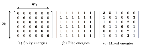
Challenges in budget allocation: Allocating the budgets is a challenging task, as each block in the spectrum of the signal may have very different energy concentration properties in time domain, or equivalently, different variations in |Z^jr|2|\widehat{Z}_{j}^{r}|^{2} as a function of rr. To see this more concretely, in Figure 1, we show three hypothetical examples of such variations, in the case that k0=2​k1=6k_{0}=2k_{1}=6 and all of the blocks have equal energy, leading to equal column sums in the matrices.
Refer to caption
Figure 1: Three hypothetical examples of matrices with (r,j)(r,j)-th entry given by |Z^jr|2|\widehat{Z}_{j}^{r}|^{2}, i.e., each row corresponds to a single sequence ZrZ^{r}, but only at the entries corresponding to the k0k_{0} blocks in XX.

In the first example, each block contributes to a different ZrZ^{r}, and thus the blocks could be located by running 11-sparse recovery separately on the 2​k12k_{1} signals. In stark contrast, in the second example, each block contributes equally to each ZrZ^{r}, so we would be much better off running k0k_{0}-sparse recovery on a single (arbitrary) ZrZ^{r}. Finally, in the third example, the best budget allocation scheme is completely unclear by inspection alone! We need to design an allocation scheme to handle all of these cases, and to do so without even knowing the structure of the matrix.

While the examples in Figure 1 may seem artificial, and are not necessarily feasible with the exact values given, we argue in Appendix E that situations exhibiting the same general behavior are entirely feasible.

Importance sampling: Our solution is to sample rr values with probability proportional to an estimate of ‖Z^r‖22\|\widehat{Z}^{r}\|_{2}^{2}, and sample sparsity budgets from a carefully defined distribution (see Section 3, Algorithm 1). We show that sufficiently accurate estimates of ‖Z^r‖22\|\widehat{Z}^{r}\|_{2}^{2} for all r∈[2​k1]r\in[2k_{1}] can be obtained using O⁡(k0​k1)O(k_{0}k_{1}) samples of XX via hashing techniques (cf., Section 4); hence, what we are essentially doing is using these samples to determine where most of the energy of the signal is located, and then favoring the parts of the signal that appear to have more energy. This is exactly the step that makes our algorithm adaptive, and we prove that it produces a total budget in (3) of the form O⁡(k0​log⁡(1+k0))O(k_{0}\log(1+k_{0})), on average.

Ideally, one would hope to solve (3) using a total budget of O⁡(k0)O(k_{0}), since there are only k0k_{0} blocks. However, the log⁡(1+k0)\log(1+k_{0}) factor is not an artifact of our analysis: We argue in Appendix E that very different techniques would be needed to remove it in general. Specifically, we design a signal XX for which the optimal solution to (3) indeed satisfies ∑r∈[2​k1]sr=Ω⁡(k0​log⁡(1+k0))\sum_{r\in[2k_{1}]}s^{r}=\Omega(k_{0}\log(1+k_{0})).

Iterative procedure and updating the residual: The techniques described above allow us to recover a list of blocks that contribute a constant fraction (e.g., 0.90.9) of the signal energy. We use O⁡(log⁡SNR)O(\log\mathrm{SNR}) iterations of our main procedure to reduce the SNR to a constant, and then achieve (1+ϵ)(1+\epsilon)-recovery with an extra “clean-up” step. Most of the techniques involved in this part are more standard, with a notable exception: Running a standard sparse FFT with budgets srs^{r} on the reduced space (i.e., on the vectors ZrZ^{r}) is not easy to implement in k0​k1​poly​(log⁡n)k_{0}k_{1}\mathrm{poly}(\log n) time when ZrZ^{r} are the residual signals. The natural approach is to subtract the current estimate χ^\widehat{\chi} of X^\widehat{X} from our samples and essentially run on the residual, but subtraction in k0​k1​poly​(log⁡n)k_{0}k_{1}\mathrm{poly}(\log n) time is not straightforward to achieve. Our solution crucially relies on a novel block semi-equispaced FFT (see Section 4.2), and the idea of letting the location primitives in the reduced space operate using common randomness (see Appendix F).

3 Location via Importance Sampling

As outlined above, our approach locates blocks by applying standard sparse FFT techniques to the downsampled signals arising from Definition 2.2. In this section, we present the techniques for assigning the corresponding sparsity budgets (cf., (3)).

We use a novel procedure called energy-based importance sampling, which approximately samples rr values with probability proportional to ‖Z^r‖2\|\widehat{Z}^{r}\|^{2}. Since these energies are not known exactly, we instead sample proportional to a general vector γ=(γ1,…,γ2​k1)\gamma=(\gamma^{1},\dotsc,\gamma^{2k_{1}}), where we think of γr\gamma^{r} as approximating ‖Z^r‖2\|\widehat{Z}^{r}\|^{2}. The techniques for obtaining these estimates are deferred to Section 4.

The details are shown in Algorithm 1, where we repeatedly sample from the distribution wqrw_{q}^{r}, corresponding to independently sampling rr proportional to γr\gamma^{r}, and qq from a truncated geometric distribution. The resulting sparsity level to apply to ZrZ^{r} is selected to be sr=10⋅2qs^{r}=10\cdot 2^{q}.

According to Definition 2.3, sr=10⋅2qs^{r}=10\cdot 2^{q} covers any given frequency jj for which |Z^jr|2≥‖Z^r‖2210⋅2q|\widehat{Z}^{r}_{j}|^{2}\geq\frac{\|\widehat{Z}^{r}\|_{2}^{2}}{10\cdot 2^{q}}. The intuition behind sampling qq proportional to 2−q2^{-q} is that this gives a high probability of producing small qq values to cover the heaviest signal components, while having a small probability of producing large qq values to cover the smaller signal components. We only want to do the latter rarely, since it costs significantly more samples.

Algorithm 1 Procedure for allocating sparsity budgets to the downsampled signals
1: procedure BudgetAllocation(γ,k0,k1,δ,p\gamma,k_{0},k_{1},\delta,p)
2:   S←∅S\leftarrow\emptyset
3:   for i∈{1,…,10δ​k0⋅log⁡1p}i\in\{1,\dotsc,\frac{10}{\delta}k_{0}\cdot\log\frac{1}{p}\} do
4:    Sample (ri,qi)∈[2​k1]×{1,…,log2⁡10​k0δ}(r_{i},q_{i})\in[2k_{1}]\times\{1,\dotsc,\log_{2}\frac{10k_{0}}{\delta}\} with probability wqr=2−q1−δ/(10​k0)​γr‖γ‖1w^{r}_{q}=\frac{2^{-q}}{1-\delta/(10k_{0})}\frac{\gamma^{r}}{\|\gamma\|_{1}}
5:    S←S∪{(ri,qi)}S\leftarrow S\cup\{(r_{i},q_{i})\}
6:   for r∈[2​k1]r\in[2k_{1}] do
7:     q∗←max(r,q′)∈S⁡{q′}q^{*}\leftarrow\max_{(r,q^{\prime})\in S}\{q^{\prime}\} ⊳\triangleright By convention, max⁡∅=−∞\max\emptyset=-\infty
8:    sr←10⋅2q∗s^{r}\leftarrow 10\cdot 2^{q^{*}}
9:   return s=[sr]r∈[2​k1]s=[s^{r}]_{r\in[2k_{1}]}

We first bound the expected total sum of budgets returned by BudgetAllocation.

Lemma 3.1.

(BudgetAllocation budget guarantees) For any integers k0k_{0} and k1k_{1}, any positive vector γ∈ℝ2​k1\gamma\in\mathbb{R}^{2k_{1}}, and any parameters p∈(0,12)p\in\big(0,\frac{1}{2}\big) and δ∈(0,1)\delta\in(0,1), if the procedure BudgetAllocation in Algorithm 1 is run with inputs (γ,k0,k1,δ,p)(\gamma,k_{0},k_{1},\delta,p), then the expected value of the total sum of budgets returned, {sr}r∈[2​k1]\{s^{r}\}_{r\in[2k_{1}]}, satisfies 𝔼⁡[∑r∈[2​k1]sr]≤200​k0δ​log⁡k0δ​log​1p\mathbb{E}\big[\sum_{r\in[2k_{1}]}s^{r}\big]\leq 200\,\frac{k_{0}}{\delta}\log\frac{k_{0}}{\delta}\log\frac{1}{p}. The runtime of the procedure is O⁡(k0δ​log⁡1p+k1)O\big(\frac{k_{0}}{\delta}\log\frac{1}{p}+k_{1}\big).

Proof.

Each time a new (r,q)(r,q) pair is sampled, the sum of the srs^{r} values increases by at most 10⋅2q10\cdot 2^{q}, and hence the overall expected sum is upper bounded by the number of trials 10​k0​log⁡1p10k_{0}\log\frac{1}{p} times the expected value of 10⋅2q10\cdot 2^{q} for a single trial:

𝔼⁡[∑r∈[2​k1]sr]≤10δk0⋅log1p∑r∈[2​k1]∑q=1log2⁡10​k0δwrq⋅10⋅2q=100​k0​log⁡1pδ⋅11−δ/(10​k0)∑q=1log2⁡10​k0δ∑r∈[2​k1]γr‖γ‖1≤200​k0δ​log⁡k0δ​log⁡1p,\begin{split}\mathbb{E}\Big[\sum_{r\in[2k_{1}]}s^{r}\Big]&\leq\frac{10}{\delta}k_{0}\cdot\log\frac{1}{p}\sum_{r\in[2k_{1}]}\sum_{q=1}^{\log_{2}\frac{10k_{0}}{\delta}}w^{r}_{q}\cdot 10\cdot 2^{q}\\ &=\frac{100k_{0}\log\frac{1}{p}}{\delta}\cdot\frac{1}{1-\delta/(10k_{0})}\sum_{q=1}^{\log_{2}\frac{10k_{0}}{\delta}}\sum_{r\in[2k_{1}]}\frac{\gamma^{r}}{\|\gamma\|_{1}}\\ &\leq 200\frac{k_{0}}{\delta}\log\frac{k_{0}}{\delta}\log\frac{1}{p},\end{split}

where the second line follows from the definition of wqrw_{q}^{r}, and the third line follows from δ10​k0≤12\frac{\delta}{10k_{0}}\leq\frac{1}{2} (since δ≤1\delta\leq 1) and ∑r∈[2​k1]γr‖γ‖1=1\sum_{r\in[2k_{1}]}\frac{\gamma^{r}}{\|\gamma\|_{1}}=1.

Runtime:

Note that sampling from wqrw_{q}^{r} amounts to sampling qq and rr values independently, and the corresponding alphabet sizes are O⁡(log⁡k0δ)O\big(\log\frac{k_{0}}{\delta}\big) and O⁡(k1)O(k_{1}) respectively. The stated runtime follows since we take O⁡(k0δ​log⁡1p)O\big(\frac{k_{0}}{\delta}\log\frac{1}{p}\big) samples, and sampling from discrete distributions can be done in time linear in the alphabet size and number of samples [HMM93]. The second loop in Algorithm 1 need not be done explicitly, since the maximum qq value can be updated after taking each sample. ∎

As we discussed in Section 2, the log⁡k0\log k_{0} term in the number of samples would ideally be avoided; however, in Appendix E.2, we argue that even the optimal solution to (3) can contain such a factor.

We now turn to formalizing the fact that the budgets returned by BudgetAllocation are such that most of the dominant blocks are found. To do this, we introduce the following notion.

Definition 3.1 (Active frequencies).

Given (n,k0,k1)(n,k_{0},k_{1}), a signal X∈ℂnX\in\mathbb{C}^{n}, a parameter δ∈(0,1)\delta\in(0,1), and a (k1,δ)(k_{1},\delta)-downsampling {Zr}r∈[2​k1]\{Z^{r}\}_{r\in[2k_{1}]} of XX, the set of active frequencies S~\tilde{S} is defined as

S~={j∈[nk1]:∑r∈[2​k1](|Z^jr|2⋅γr‖Z^r‖22)≥δ⋅∑r∈[2​k1]‖Z^r‖22k0}.\tilde{S}=\Big\{j\in\Big[\frac{n}{k_{1}}\Big]\,:\,\sum_{r\in[2k_{1}]}\Big(|\widehat{Z}^{r}_{j}|^{2}\cdot\frac{\gamma^{r}}{\|\widehat{Z}^{r}\|_{2}^{2}}\Big)\geq\delta\cdot\frac{\sum_{r\in[2k_{1}]}\|\widehat{Z}^{r}\|_{2}^{2}}{k_{0}}\Big\}. (4)

Observe that if γr=‖Z^r‖22\gamma^{r}=\|\widehat{Z}^{r}\|_{2}^{2}, this reduces to ∑r∈[2​k1]|Z^jr|2≥δ⋅∑r∈[2​k1]‖Z^r‖22k0\sum_{r\in[2k_{1}]}|\widehat{Z}^{r}_{j}|^{2}\geq\delta\cdot\frac{\sum_{r\in[2k_{1}]}\|\widehat{Z}^{r}\|_{2}^{2}}{k_{0}}, thus essentially stating that the sum of the energies over r∈[2​k1]r\in[2k_{1}] for the given block index jj is an Ω⁡(δk0)\Omega\big(\frac{\delta}{k_{0}}\big) fraction of the total energy. Combined with Lemma 2.3, this roughly amounts to ‖X^Ij‖22\|\widehat{X}_{I_{j}}\|_{2}^{2} exceeding an Ω⁡(δk0)\Omega\big(\frac{\delta}{k_{0}}\big) fraction of ‖X^‖22\|\widehat{X}\|_{2}^{2}.

To formalize and generalize this intuition, the following lemma states that the frequencies within S~\tilde{S} account for most of the energy in XX, as long as each γr\gamma^{r} approximates ‖Z^r‖22\|\widehat{Z}^{r}\|_{2}^{2} sufficiently well.

Lemma 3.2.

(Properties of active frequencies) Fix (n,k0,k1)(n,k_{0},k_{1}), a parameter δ∈(0,120)\delta\in\big(0,\frac{1}{20}\big), a signal X∈ℂnX\in\mathbb{C}^{n}, and a (k1,δ)(k_{1},\delta)-downsampling {Zr}r∈[2​k1]\{Z^{r}\}_{r\in[2k_{1}]} of XX. Moreover, fix an arbitrary set S∗⊆[nk1]S^{*}\subseteq\big[\frac{n}{k_{1}}\big] of cardinality at most 10​k010k_{0}, and a vector γ∈ℝ2​k1\gamma\in\mathbb{R}^{2k_{1}} satisfying

∑r∈[2​k1]|‖Z^S∗r‖22−γr|+≤40​δ​∑r∈[2​k1]‖Z^r‖22.\displaystyle\sum_{r\in[2k_{1}]}\Big|\|\widehat{Z}^{r}_{S^{*}}\|_{2}^{2}-\gamma^{r}\Big|_{+}\leq 40\delta\sum_{r\in[2k_{1}]}\|\widehat{Z}^{r}\|_{2}^{2}. (*)

Fix the set of active frequencies S~\tilde{S} according to Definition 4, and define the signal X^S~\widehat{X}_{\tilde{S}} to equal X^\widehat{X} on all intervals {Ij;j∈S~}\{I_{j}\,;j\in\tilde{S}\} (see Definition 1.1), and zero elsewhere. Then ‖X^S∗\S~‖22≤100​δ​‖X^‖22\|\widehat{X}_{S^{*}\backslash\tilde{S}}\|_{2}^{2}\leq 100\sqrt{\delta}\|\widehat{X}\|_{2}^{2}.

The proof of Lemma 3.2 is given in Appendix B.1.

What remains is to show that if jj is active, then jj is covered by some srs^{r} in Z^r\widehat{Z}^{r} with high constant probability upon running Algorithm 1. This is formulated in the following.

Lemma 3.3.

(BudgetAllocation covering guarantees) Fix (n,k0,k1)(n,k_{0},k_{1}), the parameters δ∈(0,1)\delta\in(0,1) and p∈(0,12)p\in\big(0,\frac{1}{2}\big), a signal X∈ℂnX\in\mathbb{C}^{n}, and a (k1,δ)(k_{1},\delta)-downsampling {Zr}r∈[2​k1]\{Z^{r}\}_{r\in[2k_{1}]} of XX. Moreover, fix a vector γ∈ℝ2​k1\gamma\in\mathbb{R}^{2k_{1}} satisfying

‖γ‖1≤10​∑r∈[2​k1]‖Z^r‖22.\|\gamma\|_{1}\leq 10\sum_{r\in[2k_{1}]}\|\widehat{Z}^{r}\|_{2}^{2}. (5)

Suppose that BudgetAllocation in Algorithm 1 is run with inputs (γ,k0,k1,δ,p)(\gamma,k_{0},k_{1},\delta,p), and outputs the budgets {sr}r∈[2​k1]\{s^{r}\}_{r\in[2k_{1}]}. Then for any active jj (i.e., j∈S~j\in\tilde{S} as per Definition 3.1), the probability that there exists some r∈[2​k1]r\in[2k_{1}] such that jj is covered by srs^{r} in Z^r\widehat{Z}^{r} is at least 1−p1-p.

Proof.

Recall from Definition 2.3 that if a pair (r,q)(r,q) is sampled in the first loop of BudgetAllocation, then jj is covered provided that |Z^jr|2≥‖Z^r‖2210⋅2q.|\widehat{Z}^{r}_{j}|^{2}\geq\frac{\|\widehat{Z}^{r}\|_{2}^{2}}{10\cdot 2^{q}}. We therefore define

qjr=min⁡{q∈ℤ+:|Z^jr|2≥‖Z^r‖2210⋅2q},q_{j}^{r}=\min\bigg\{q\in\mathbb{Z}_{+}\,:\,|\widehat{Z}_{j}^{r}|^{2}\geq\frac{\|\widehat{Z}^{r}\|_{2}^{2}}{10\cdot 2^{q}}\bigg\}, (6)

and note that the event described in the lemma statement is equivalent to some pair (r,q)(r,q) being sampled with qjr≤qq^{r}_{j}\leq q. Note that due to the range of qq from which we sample (cf., Algorithm 1), this can only occur if qjr≤log2⁡10​k0δq^{r}_{j}\leq\log_{2}\frac{10k_{0}}{\delta}.

Taking a single sample: We first compute the probability of being covered for a single random sample of (q,r)(q,r), denoting the corresponding probability by ℙ1​[⋅]\mathbb{P}_{1}[\cdot]. Recalling from line 4 of Algorithm 1 that we sample each (q,r)(q,r) with probability wqr=2−q1−δ/(10​k0)​γr‖γ‖1w_{q}^{r}=\frac{2^{-q}}{1-\delta/(10k_{0})}\frac{\gamma^{r}}{\|\gamma\|_{1}}, we obtain

ℙ1​[j​ covered]\displaystyle\mathbb{P}_{1}[j\text{ covered}] =∑r∈[2​k1]∑qjr≤q≤log2⁡10​k0δwqr\displaystyle=\sum_{r\in[2k_{1}]}\sum_{q^{r}_{j}\leq q\leq\log_{2}\frac{10k_{0}}{\delta}}w_{q}^{r}
=11−δ/(10​k0)​∑r∈[2​k1]∑qjr≤q≤log2⁡10​k0δ2−q​γr‖γ‖1\displaystyle=\frac{1}{1-\delta/(10k_{0})}\sum_{r\in[2k_{1}]}\sum_{q^{r}_{j}\leq q\leq\log_{2}\frac{10k_{0}}{\delta}}2^{-q}\frac{\gamma^{r}}{\|\gamma\|_{1}}
≥12∑r∈[2​k1]:qjr≤log2⁡10​k0δ2−qjrγr‖γ‖1\displaystyle\geq\frac{1}{2}\sum_{r\in[2k_{1}]\,:\,q_{j}^{r}\leq\log_{2}\frac{10k_{0}}{\delta}}2^{-q_{j}^{r}}\frac{\gamma^{r}}{\|\gamma\|_{1}}
=12∑r∈[2​k1]2−qjrγr‖γ‖1−12∑r∈[2​k1]:qjr>log2⁡10​k0δ2−qjrγr‖γ‖1,\displaystyle=\frac{1}{2}\sum_{r\in[2k_{1}]}2^{-q_{j}^{r}}\frac{\gamma^{r}}{\|\gamma\|_{1}}-\frac{1}{2}\sum_{r\in[2k_{1}]\,:\,q_{j}^{r}>\log_{2}\frac{10k_{0}}{\delta}}2^{-q_{j}^{r}}\frac{\gamma^{r}}{\|\gamma\|_{1}}, (7)

where the third line follows since δ/(10​k0)≤12\delta/(10k_{0})\leq\frac{1}{2} due to the assumption that δ≤1\delta\leq 1.

Bounding the first term in (7): Observe from (6) that 2−qjr≥12​10​|Z^jr|2‖Z^r‖222^{-q_{j}^{r}}\geq\frac{1}{2}\frac{10|\widehat{Z}_{j}^{r}|^{2}}{\|\widehat{Z}^{r}\|_{2}^{2}}, and recall the definition of being active in (4). Combining these, we obtain the following when jj is active:

12​∑r∈[2​k1]2−qjr​γr‖γ‖1≥104​‖γ‖1​∑r∈[2​k1]|Z^jr|2​γr‖Z^r‖22≥10​δ4​‖γ‖1⋅∑r∈[2​k1]‖Z^r‖22k0≥δ4​k0,\begin{split}\frac{1}{2}\sum_{r\in[2k_{1}]}2^{-q_{j}^{r}}\frac{\gamma^{r}}{\|\gamma\|_{1}}&\geq\frac{10}{4\|\gamma\|_{1}}\sum_{r\in[2k_{1}]}\frac{|\widehat{Z}_{j}^{r}|^{2}\gamma^{r}}{\|\widehat{Z}^{r}\|_{2}^{2}}\\ &\geq\frac{10\delta}{4\|\gamma\|_{1}}\cdot\frac{\sum_{r\in[2k_{1}]}\|\widehat{Z}^{r}\|_{2}^{2}}{k_{0}}\geq\frac{\delta}{4k_{0}},\end{split}

where the last inequality follows from the assumption on ‖γ‖1\|\gamma\|_{1} in the lemma statement.

Bounding the second term in (7): We have

12∑r∈[2​k1]:qjr>log2⁡10​k0δ2−qjrγr‖γ‖1≤12​∑r∈[2​k1]δ10​k0​γr‖γ‖1=δ20​k0.\begin{split}\frac{1}{2}\sum_{r\in[2k_{1}]\,:\,q_{j}^{r}>\log_{2}\frac{10k_{0}}{\delta}}2^{-q_{j}^{r}}\frac{\gamma^{r}}{\|\gamma\|_{1}}&\leq\frac{1}{2}\sum_{r\in[2k_{1}]}\frac{\delta}{10k_{0}}\frac{\gamma^{r}}{\|\gamma\|_{1}}=\frac{\delta}{20k_{0}}.\end{split}

Hence, we deduce from (7) that ℙ1​[j​ covered]≥δ5​k0\mathbb{P}_{1}[j\text{ covered}]\geq\frac{\delta}{5k_{0}}.

Taking multiple independent samples: Since the sampling is done 10δ​k0⋅log⁡1p\frac{10}{\delta}k_{0}\cdot\log\frac{1}{p} times independently, the overall probability of an active block jj being covered satisfies

ℙ⁡[j​ covered]≥1−(1−δ5​k0)10δ​k0⋅log⁡1p≥1−exp(−105⋅log1p)≥1−p,\begin{split}\mathbb{P}[j\text{ covered}]&\geq 1-\bigg(1-\frac{\delta}{5k_{0}}\bigg)^{\frac{10}{\delta}k_{0}\cdot\log\frac{1}{p}}\geq 1-\exp\bigg(-\frac{10}{5}\cdot\log\frac{1}{p}\bigg)\geq 1-p,\end{split}

where we have applied the inequality 1−ζ≤e−ζ1-\zeta\leq e^{-\zeta} for ζ≥0\zeta\geq 0. ∎

3.1 The Complete Location Algorithm

In Algorithm 2, we give the details of MultiBlockLocate, which performs the above-described energy-based importance sampling procedure, runs the sparse FFT location algorithm (see Appendix F) with the resulting budgets, and returns a list LL containing the block indices that were identified.

MultiBlockLocate calls two primitives that are defined later in the paper, but their precise details are not needed in order to understand the location step:

  • •

    EstimateEnergies (see Section 4.4) provides us with a vector γ\gamma providing a good approximation of each ‖Z^r‖22\|\widehat{Z}^{r}\|_{2}^{2}, in the sense of satisfying the preconditions of Lemmas 3.2 and 3.3;

  • •

    LocateReducedSignals (see Appendix F) accepts the sparsity budgets {sr}\{s^{r}\} and runs a standard srs^{r}-sparse fast FFT algorithm on each downsampled signal ZrZ^{r} in order to locate the dominant frequencies.

Note that in addition to XX, these procedures accept a second signal χ^\widehat{\chi}; this becomes relevant when we iteratively run the block sparse FFT (cf., Section 5), representing previously-estimated components that are subtracted off to produce a residual.

The required guarantees on LocateReducedSignals are given in Lemma 2.4 (and more formally in Appendix E.2), and in order to prove our main result on MultiBlockLocate, we also need the following lemma ensuring that we can compute energy estimates satisfying the preconditions of Lemmas 3.2 and 3.3; the procedure and proof are presented in Section 4.4.

Lemma 3.4.

(EstimateEnergies guarantees) Given (n,k0,k1)(n,k_{0},k_{1}), the signals X∈ℂnX\in\mathbb{C}^{n} and χ^∈ℂn\widehat{\chi}\in\mathbb{C}^{n} with ‖X^−χ^‖22≥1poly⁡(n)​‖χ^‖2\|\widehat{X}-\widehat{\chi}\|_{2}^{2}\geq\frac{1}{\mathrm{poly}(n)}\|\widehat{\chi}\|_{2}, and the parameter δ∈(1n,120)\delta\in\big(\frac{1}{n},\frac{1}{20}\big), the procedure EstimateEnergies(X,χ^,n,k0,k1CLOSE(X,\widehat{\chi},n,k_{0},k_{1},𝑂𝑃𝐸𝑁δ)\delta) returns a vector γ∈ℝ2​k1\gamma\in\mathbb{R}^{2k_{1}} such that, for any given set S∗S^{*} of cardinality at most 10​k010k_{0}, we have the following with probability at least 12\frac{1}{2}:

  1. 1.

    ∑r∈[2​k1]|‖Z^S∗r‖22−γr|+≤40​δ​∑r∈[2​k1]‖Z^r‖22\sum_{r\in[2k_{1}]}\Big|\|\widehat{Z}^{r}_{S^{*}}\|_{2}^{2}-\gamma^{r}\Big|_{+}\leq 40\delta\sum_{r\in[2k_{1}]}\|\widehat{Z}^{r}\|_{2}^{2};

  2. 2.

    ‖γ‖1≤10​∑r∈[2​k1]‖Z^r‖22\|\gamma\|_{1}\leq 10\sum_{r\in[2k_{1}]}\|\widehat{Z}^{r}\|_{2}^{2};

where {Zr}r∈[2​k1]\{Z^{r}\}_{r\in[2k_{1}]} is the (k1,δ)(k_{1},\delta)-downsampling of X−χX-\chi (see Definition 2.2).

Moreover, if χ^\widehat{\chi} is (O⁡(k0),k1)(O(k_{0}),k_{1})-block sparse, then the sample complexity is O⁡(k0​k1δ2​log⁡1δ​log​1δ​p)O(\frac{k_{0}k_{1}}{\delta^{2}}\log\frac{1}{\delta}\log\frac{1}{\delta p}), and the runtime is O⁡(k0​k1δ2​log2​1δ​log2​n)O(\frac{k_{0}k_{1}}{\delta^{2}}\log^{2}\frac{1}{\delta}\log^{2}n).

Remark 3.1.

The preceding lemma ensures that the γr\gamma^{r} provide good approximations of ‖Z^r‖22\|\widehat{Z}^{r}\|_{2}^{2} in a “restricted” and “one-sided” sense, while not over-estimating the total energy by more than a constant factor. Specifically, the first part concerns the energy of Z^r\widehat{Z}^{r} restricted to a fixed set of size O⁡(k0)O(k_{0}), and characterizes the extent to which the energies are under-estimated. It appears to be infeasible to characterize over-estimation in the same way (e.g., replacing |⋅|+|\cdot|_{+} by |⋅||\cdot|), since several of the samples could be overly large due to spiky noise.

Remark 3.2.

Here and subsequently, the poly⁡(n)\mathrm{poly}(n) lower bounds regarding (X^,χ^)(\widehat{X},\widehat{\chi}) are purely technical, resulting from extremely small errors when subtracting off χ^\widehat{\chi}. See Section 4.2 for further details.

Algorithm 2 Multi-block sparse location
1: procedure MultiBlockLocate(X,χ^,n,k0,k1,δ,pX,\widehat{\chi},n,k_{0},k_{1},\delta,p)
2:   for t∈{1,…,10​log⁡1p}t\in\{1,\dotsc,10\log\frac{1}{p}\} do
3:    γ←EstimateEnergies​(X,χ^,n,k0,k1,δ)\gamma\leftarrow\textsc{EstimateEnergies}(X,\widehat{\chi},n,k_{0},k_{1},\delta) ⊳\triangleright See Section 4.4
4:    𝐬(t)←BudgetAllocation​(γ,k0,k1,δ,12​δ​p)\mathbf{s}^{(t)}\leftarrow\textsc{BudgetAllocation}(\gamma,k_{0},k_{1},\delta,\frac{1}{2}\delta p) ⊳\triangleright γ=(γ1,…,γ2​k1)\gamma=(\gamma^{1},\dotsc,\gamma^{2k_{1}})   
5:   𝐬←maxt⁡𝐬(t)\mathbf{s}\leftarrow\max_{t}\mathbf{s}^{(t)} (element-wise with respect to r∈[2​k1]r\in[2k_{1}])
6:   L←LocateReducedSignals​(X,χ^,n,k0,k1,s,δ,12​δ​p)L\leftarrow\textsc{LocateReducedSignals}(X,\widehat{\chi},n,k_{0},k_{1},\textbf{s},\delta,\frac{1}{2}\delta p) ⊳\triangleright See Appendix F
7:   return LL

We are now in a position to provide our guarantees on MultiBlockLocate, namely, on the behavior of the list size, and on the energy that the components in the list capture. Note that the output of MultiBlockLocate is random, since the same is true of EstimateEnergies, BudgetAllocation, and LocateReducedSignals.

Lemma 3.5.

(MultiBlockLocate guarantees) Given (n,k0,k1)(n,k_{0},k_{1}), the parameters δ∈(1n,120)\delta\in\big(\frac{1}{n},\frac{1}{20}\big) and p∈(1n,12)p\in\big(\frac{1}{n},\frac{1}{2}\big), and the signals X∈ℂnX\in\mathbb{C}^{n} and χ∈ℂn\chi\in\mathbb{C}^{n} with χ^0\widehat{\chi}_{0} uniformly distributed over an arbitrarily length-‖χ^‖2poly⁡(n)\frac{\|\widehat{\chi}\|^{2}}{\mathrm{poly}(n)} interval, the output LL of the function MultiBlockLocate(X,X^,k1,k0,n,δ,p)(X,\widehat{X},k_{1},k_{0},n,\delta,p) has the following properties for any set S∗S^{*} of cardinality at most 10​k010k_{0}:

  1. 1.

    𝔼⁡[|L|]=O⁡(k0δ​log⁡k0δ​log​1p​log2​1δ​p)\mathbb{E}\big[|L|\big]=O\big(\frac{k_{0}}{\delta}\log\frac{k_{0}}{\delta}\log\frac{1}{p}\log^{2}\frac{1}{\delta p}\big);

  2. 2.

    ∑j∈S∗\L‖(X^−χ^)Ij‖22≤200​δ​‖X^−χ^‖22\sum_{j\in S^{*}\backslash L}\|(\widehat{X}-\widehat{\chi})_{I_{j}}\|_{2}^{2}\leq 200\sqrt{\delta}\|\widehat{X}-\widehat{\chi}\|_{2}^{2} with probability at least 1−p1-p.

Moreover, if χ^\widehat{\chi} is (O⁡(k0),k1)(O(k_{0}),k_{1})-block sparse, and we have δ=Ω⁡(1poly⁡(log⁡n))\delta=\Omega\big(\frac{1}{\mathrm{poly}(\log n)}\big) and p=Ω⁡(1poly⁡(log⁡n))p=\Omega\big(\frac{1}{\mathrm{poly}(\log n)}\big), then (i) the expected sample complexity is O∗​(k0δ​log⁡(1+k0)​log​n+k0​k1δ2)O^{*}\big(\frac{k_{0}}{\delta}\log(1+k_{0})\log n+\frac{k_{0}k_{1}}{\delta^{2}}\big), and the expected runtime is O∗​(k0δ​log⁡(1+k0)​log2​n+k0​k1δ2​log2​n+k0​k1δ​log3​n)O^{*}\big(\frac{k_{0}}{\delta}\log(1+k_{0})\log^{2}n+\frac{k_{0}k_{1}}{\delta^{2}}\log^{2}n+\frac{k_{0}k_{1}}{\delta}\log^{3}n\big); (ii) if the procedure returns LL, then we are guaranteed that the algorithm used O∗​(|L|⋅log⁡n+k0​k1δ2)O^{*}\big(|L|\cdot\log n+\frac{k_{0}k_{1}}{\delta^{2}}\big) samples and O∗​(|L|⋅log2⁡n+k0​k1δ2​log2​n+k0​k1δ​log3​n)O^{*}\big(|L|\cdot\log^{2}n+\frac{k_{0}k_{1}}{\delta^{2}}\log^{2}n+\frac{k_{0}k_{1}}{\delta}\log^{3}n\big) runtime.

Remark 3.1.

The procedure MultiBlockLocate is oblivious to the choice of S∗S^{*} in this lemma statement.

Proof.

First claim: Note that in each iteration of the outer loop when we run BudgetAllocation(γ,k0,k1,δ,12​δ​p)(\gamma,k_{0},k_{1},\delta,\frac{1}{2}\delta p), Lemma 3.1 implies that for any tt, the following holds true:

𝔼⁡[∑r∈[2​k1]sr(t)]=O⁡(k0δ​log⁡k0δ​log​1δ​p),\mathbb{E}\Big[\sum_{r\in[2k_{1}]}\textbf{s}^{(t)}_{r}\Big]=O\Big(\frac{k_{0}}{\delta}\log\frac{k_{0}}{\delta}\log\frac{1}{\delta p}\Big),

where sr(t)\textbf{s}^{(t)}_{r} is the rr-th entry of the budget allocation vector 𝐬t\mathbf{s}^{t} at iteration tt. Therefore,

𝔼⁡[∑r∈[2​k1]sr]=𝔼⁡[∑r∈[2​k1]maxt=1,…,10​log⁡1p⁡srt]≤∑t=110​log⁡1p𝔼⁡[∑r∈[2​k1]𝐬r(t)]=O⁡(k0​log​k0δ​log​1p​log​1δ​p).\mathbb{E}\Big[\sum_{r\in[2k_{1}]}\textbf{s}_{r}\Big]=\mathbb{E}\Big[\sum_{r\in[2k_{1}]}\max_{t=1,\dotsc,10\log\frac{1}{p}}\textbf{s}_{r}^{t}\Big]\leq\sum_{t=1}^{10\log\frac{1}{p}}\mathbb{E}\Big[\sum_{r\in[2k_{1}]}\mathbf{s}_{r}^{(t)}\Big]=O\Big(k_{0}\log\frac{k_{0}}{\delta}\log\frac{1}{p}\log\frac{1}{\delta p}\Big). (8)

We now apply Lemma 2.4, which is formalized in Appendix F; the assumption maxr∈[2​k1]⁡sr=O⁡(k0δ)\max_{r\in[2k_{1}]}\textbf{s}_{r}=O\big(\frac{k_{0}}{\delta}\big) therein is satisfied due to the range of qq from which we sample in BudgetAllocation. We set the target success probability to 1−12​δ​p1-\frac{1}{2}\delta p, which guarantees that the size of the list returned by the function LocateReducedSignals is O⁡(∑r∈[2​k1]sr​log⁡1δ​p)O\big(\sum_{r\in[2k_{1}]}\textbf{s}_{r}\log\frac{1}{\delta p}\big). Therefore, by (8), we have

𝔼⁡[|L|]=O⁡(k0δ​log⁡k0δ​log​1p​log2​1δ​p),\mathbb{E}[|L|]=O\Big(\frac{k_{0}}{\delta}\log\frac{k_{0}}{\delta}\log\frac{1}{p}\log^{2}\frac{1}{\delta p}\Big),

yielding the first statement of the lemma.

Second claim: Let X′=X−χX^{\prime}=X-\chi, and consider the set S∗S^{*} given in the lemma statement, and an arbitrary iteration tt. By Lemma 3.4 in Section 4.4 (also stated above), the approximate energy vector γ\gamma in any given iteration of the outer loop satisfies

∑r∈[2​k1]|‖Z^S∗r‖22−γr|+≤40​δ​∑r∈[2​k1]‖Z^r‖22\displaystyle\sum_{r\in[2k_{1}]}\Big|\|\widehat{Z}^{r}_{{S}^{*}}\|_{2}^{2}-\gamma^{r}\Big|_{+}\leq 40\delta\sum_{r\in[2k_{1}]}\|\widehat{Z}^{r}\|_{2}^{2}
‖γ‖1≤10​∑r∈[2​k1]‖Z^r‖22\displaystyle\|\gamma\|_{1}\leq 10\sum_{r\in[2k_{1}]}\|\widehat{Z}^{r}\|_{2}^{2} (9)

with probability at least 12\frac{1}{2}. When this is the case, the vector γ\gamma meets the requirements of Lemmas 3.2 and 3.3. That means that the probability of having an energy estimate γ\gamma that meets these requirements in at least one iteration is lower bounded by 1−(12)10​log⁡1p≥1−p1-(\frac{1}{2})^{10\log\frac{1}{p}}\geq 1-p.

We now consider an arbitrary iteration in which the above conditions on γ\gamma are satisfied. We write

∑j∈S∗\L‖X^Ij′‖22=∑j∈(S∗∩S~)\L‖X^Ij′‖22+∑j∈S∗\(S~∪L)‖X^Ij′‖22.\displaystyle\sum_{j\in S^{*}\backslash L}\|\widehat{X}^{\prime}_{I_{j}}\|_{2}^{2}=\sum_{j\in(S^{*}\cap\tilde{S})\backslash L}\|\widehat{X}^{\prime}_{I_{j}}\|_{2}^{2}+\sum_{j\in S^{*}\backslash(\tilde{S}\cup L)}\|\widehat{X}^{\prime}_{I_{j}}\|_{2}^{2}. (10)

The second term is bounded by

∑j∈S∗\(S~∪L)‖X^Ij′‖22≤∑j∈S∗\S~‖X^Ij′‖22≤100​δ​‖X^′‖22\sum_{j\in S^{*}\backslash(\tilde{S}\cup L)}\|\widehat{X}^{\prime}_{I_{j}}\|_{2}^{2}\leq\sum_{j\in S^{*}\backslash\tilde{S}}\|\widehat{X}^{\prime}_{I_{j}}\|_{2}^{2}\leq 100\sqrt{\delta}\|\widehat{X}^{\prime}\|_{2}^{2} (11)

by Lemma 3.2, which uses the first condition on γ\gamma in (9).

We continue by calculating the expected value of the first term in (10) with respect to the randomness of BudgetAllocation and LocateReducedSignals:

𝔼⁡[∑j∈(S∗∩S~)\L‖X^Ij′‖22]\displaystyle\mathbb{E}\Big[\sum_{j\in(S^{*}\cap\tilde{S})\backslash L}\|\widehat{X}^{\prime}_{I_{j}}\|_{2}^{2}\Big] =𝔼[∑j∈(S∗∩S~)∥X^Ij′∥22ℐ[j∉L]]\displaystyle=\mathbb{E}\Big[\sum_{j\in(S^{*}\cap\tilde{S})}\|\widehat{X}^{\prime}_{I_{j}}\|_{2}^{2}\mathcal{I}\big[j\notin L\big]\Big]
≤∑j∈S~∥X^Ij′∥22⋅ℙ[j∉L].\displaystyle\leq\sum_{j\in\tilde{S}}\|\widehat{X}^{\prime}_{I_{j}}\|_{2}^{2}\cdot\mathbb{P}\big[j\notin L\big]. (12)

We thus consider the probability ℙ[j∉L]\mathbb{P}[j\notin L] for an arbitrary j∈S~j\in\tilde{S}. If j∈S~j\in\tilde{S}, then by Lemma 3.3 and the choice of the final parameter of 12​δ​p\frac{1}{2}\delta p passed to BudgetAllocation, there is at least one r∈[2​k1]r\in[2k_{1}] such that jj is covered, with probability at least 1−12​δ​p1-\frac{1}{2}\delta p. We also know from Lemma 2.4 that the failure probability of LocateReducedSignals for some covered jj is at most 12​δ​p\frac{1}{2}\delta p. A union bound on these two events gives

ℙ[j∉L]≤δp,∀j∈S~.\mathbb{P}\big[j\notin L\big]\leq\delta p,\quad\forall j\in\tilde{S}.

Hence, we deduce from (12) that

𝔼⁡[∑j∈(S∗∩S~)\L‖X^Ij′‖22]≤δ​p⋅‖X^′‖22,\mathbb{E}\Big[\sum_{j\in(S^{*}\cap\tilde{S})\backslash L}\|\widehat{X}^{\prime}_{I_{j}}\|_{2}^{2}\Big]\leq\delta p\cdot\|\widehat{X}^{\prime}\|_{2}^{2},

and Markov’s inequality gives

∑j∈(S∗∩S~)\L‖X^Ij′‖22≤δ⋅‖X^′‖22\sum_{j\in(S^{*}\cap\tilde{S})\backslash L}\|\widehat{X}^{\prime}_{I_{j}}\|_{2}^{2}\leq\delta\cdot\|\widehat{X}^{\prime}\|_{2}^{2}

with probability at least 1−p1-p. Combining this with (10)–(11), and using the assumption δ≤120\delta\leq\frac{1}{20} to write δ≤100​δ\delta\leq 100\sqrt{\delta}, we complete the proof.

Sample complexity and runtime: We first consider the sample complexity and runtime as a function of the output LL.

There are two operations that cost us samples. The first is the call to EstimateEnergies, which costs O⁡(k0​k1δ2​log2​1δ)O(\frac{k_{0}k_{1}}{\delta^{2}}\log^{2}\frac{1}{\delta}) by Lemma 3.4. The second is the call to LocateReducedSignals; by Lemma 2.4 in Appendix F, with δ​p\delta p in place of pp, this costs O⁡(∑r∈[2​k1]sr​log⁡1δ​p​log⁡1δ​log​n)O\big(\sum_{r\in[2k_{1}]}s^{r}\log\frac{1}{\delta p}\log\frac{1}{\delta}\log n\big) samples (recall that χ^\widehat{\chi} is (O⁡(k0),k1)(O(k_{0}),k_{1})-block sparse by assumption), which is O⁡(|L|​log⁡1δ​p​log⁡1δ​log​n)O\big(|L|\log\frac{1}{\delta p}\log\frac{1}{\delta}\log n\big). Adding these contributions gives the desired result; the log⁡1p\log\frac{1}{p} and log⁡1δ\log\frac{1}{\delta} factors are hidden in the O∗​(⋅)O^{*}(\cdot) notation, since we have assumed that δ\delta and pp behave as Ω⁡(1poly​log⁡n)\Omega\big(\frac{1}{\mathrm{poly}\log n}\big).

The time complexity follows by the a similar argument, with EstimateEnergies costing O⁡(k0​k1δ2​log2​1δ​log2​n)O(\frac{k_{0}k_{1}}{\delta^{2}}\log^{2}\frac{1}{\delta}\log^{2}n) by Lemma 3.4, and the call to LocateReducedSignals costing O⁡(|L|​log⁡1δ​p​log​1δ​log2​n+k0​k1δ​log​1δ​p​log3​n)O\big(|L|\log\frac{1}{\delta p}\log\frac{1}{\delta}\log^{2}n+\frac{k_{0}k_{1}}{\delta}\log\frac{1}{\delta p}\log^{3}n\big) by Lemma 2.4 in Appendix F. The complexity of EstimateEnergies dominates that of calling BudgetAllocation, which is O⁡(k1+k0δ​log⁡1p)O\big(k_{1}+\frac{k_{0}}{\delta}\log\frac{1}{p}\big) by Lemma 3.1.

The expected sample complexity and runtime follow directly from those depending on LL, by simply substituting the expectation of |L||L| given in the lemma statement. ∎

4 Energy Estimation

In this section, we provide the energy estimation procedure used in the MultiBlockLocate procedure in Algorithm 2, and prove its guarantees that were used in the proof of Lemma 3.5. To do this, we introduce a variety of tools needed, including hashing and the semi-equispaced FFT. While such techniques are well-established for the standard sparsity setting [IKP14], applying the existing semi-equispaced FFT algorithms separately for each ZrZ^{r} in our setting would lead to a runtime of k0​k12​poly​(log⁡n)k_{0}k_{1}^{2}\mathrm{poly}(\log n). Our techniques allow us to compute the required FFT values for all rr in k0​k1​poly​(log⁡n)k_{0}k_{1}\mathrm{poly}(\log n) time, as we detail in Section 4.2.

4.1 Hashing Techniques

The notion of hashing plays a central role in our estimation primitives, and in turn makes use of random permutations.

Definition 4.1 (Approximately pairwise-independent permutation).

Fix nn, and let π:[n]→[n]\pi\,:\,[n]\to[n] be a random permutation. We say that π\pi is approximately pairwise-independent if, for any i,i′∈[n]i,i^{\prime}\in[n] and any integer tt, we have ℙ[|π(i)−π(i′)|≤t]≤4​tn\mathbb{P}[|\pi(i)-\pi(i^{\prime})|\leq t]\leq\frac{4t}{n}.

It is well known that such permutations exist in the form of a simple modulo-nn multiplication; we will specifically use the following lemma from [IK14].

Lemma 4.1.

(Choice of permutation [IK14, Lemma 3.2]) Let nn be a power of two, and define π⁡(i)=σ⋅i\pi(i)=\sigma\cdot i, where σ\sigma is chosen uniformly at random from the odd numbers in [n][n]. Then π\pi is an approximately pairwise-independent random permutation.

We now turn to the notion of hashing a signal into buckets. We do this by applying the random permutation from Lemma 4.1 along with a random shift in time domain, and then applying a suitable filter according to Definition 2.1.

Definition 4.2 (Hashing).

Given integers (n,B)(n,B), parameters σ,Δ∈[n]\sigma,\Delta\in[n], and the signals X∈ℂnX\in\mathbb{C}^{n} and G∈ℂnG\in\mathbb{C}^{n}, we say that U∈ℂBU\in\mathbb{C}^{B} is an (n,B,G,σ,Δ)(n,B,G,\sigma,\Delta)-hashing of XX if

Ub=Bn​∑i∈[nB]Xσ⁡(Δ+j+B⋅i)​Gj+B⋅i,j∈[B].U_{b}=\frac{B}{n}\sum_{i\in[\frac{n}{B}]}X_{\sigma(\Delta+j+B\cdot i)}G_{j+B\cdot i},\quad j\in[B]. (13)

Moreover, we define the following quantities:

  • •

    π⁡(j)=σ⋅j\pi(j)=\sigma\cdot j, representing the approximately pairwise random permutation;

  • •

    h⁡(j)=round⁡(j​Bn)h(j)=\mathrm{round}\big(j\frac{B}{n}\big), representing the bucket in [B][B] into which a frequency jj hashes;

  • •

    oj​(j′)=π⁡(j′)−h⁡(j)​nBo_{j}(j^{\prime})=\pi(j^{\prime})-h(j)\frac{n}{B}, representing the offset associated with two frequencies (j,j′)(j,j^{\prime}).

With these definitions, we have the following lemma, proved in Appendix C.1. Note that here we write the exact Fourier transform of UU as U^∗\widehat{U}^{*}, since later we will use U^\widehat{U} for its near-exact counterpart to simplify notation.

Lemma 4.2.

(Fourier transform of hashed signal) Fix (n,B)(n,B) and the signals X∈ℂnX\in\mathbb{C}^{n} and G∈ℂnG\in\mathbb{C}^{n} with the latter symmetric about zero. If UU is an (n,B,G,σ,Δ)(n,B,G,\sigma,\Delta)-hashing of XX, then its exact Fourier transform U^∗\widehat{U}^{*} is given by

U^b∗=∑f∈[n]X^f​G^σ​f−b​nB​ωnσ​Δ​f,b∈[B].\widehat{U}^{*}_{b}=\sum_{f\in[n]}\widehat{X}_{f}\widehat{G}_{\sigma f-b\frac{n}{B}}\omega_{n}^{\sigma\Delta f},\quad b\in[B].

We conclude this subsection by stating the following technical lemma regarding approximately pairwise independent permutations and flat filters.

Lemma 4.3.

(Additional filter property) Fix nn, and let GG be an (n,B,F)(n,B,F)-flat filter. Let π⁡(⋅)\pi(\cdot) be an approximately pairwise-independent random permutation (cf., Definition 4.1), and for f,f′∈[n]f,f^{\prime}\in[n], define of​(f′)=π⁡(f′)−nB​round​(π⁡(f)​Bn)o_{f}(f^{\prime})=\pi(f^{\prime})-\frac{n}{B}\mathrm{round}\big(\pi(f)\frac{B}{n}\big). Then for any x∈ℂnx\in\mathbb{C}^{n} and f∈[n]f\in[n], we have

∑f′≠f|X^f′|2​𝔼π​[|G^of​(f′)|2]≤10B​‖X^‖2.\sum_{f^{\prime}\neq f}|\widehat{X}_{f^{\prime}}|^{2}\mathbb{E}_{\pi}\big[|\widehat{G}_{o_{f}(f^{\prime})}|^{2}\big]\leq\frac{10}{B}\|\widehat{X}\|^{2}. (14)

The proof is given in Appendix C.2.

4.2 Semi-Equispaced FFT

Algorithm 3 Semi-equispaced inverse FFT for approximating the inverse Fourier transform, with standard sparsity (top) and block sparsity (bottom)
1: procedure SemiEquiInverseFFT(X^,n,k,ζ\widehat{X},n,k,\zeta)
2:   G^←Filter​(n,k,ζ)\widehat{G}\leftarrow\textsc{Filter}(n,k,\zeta) ⊳\triangleright See [IKP14, Sec. 12]; same as proof of Lemma 4.5
3:   Y^i←(X^⋆G^)i​n2​k\widehat{Y}_{i}\leftarrow(\widehat{X}\star\widehat{G})_{\frac{in}{2k}} for each i∈[2​k]i\in[2k]
4:   Y←InverseFFT​(Y^){Y}\leftarrow\textsc{InverseFFT}(\widehat{Y})
5:   return {Yj}|j|≤k2\{{Y}_{j}\}_{|j|\leq\frac{k}{2}}
6: procedure SemiEquiInverseBlockFFT(X^,n,k0,k1,c\widehat{X},n,k_{0},k_{1},c)
7:   G^←Filter​(n,k1,n−c)\widehat{G}\leftarrow\textsc{Filter}(n,k_{1},n^{-c}) ⊳\triangleright See proof of Lemma 4.5
8:   for j∈[2​nk1]j\in\big[\frac{2n}{k_{1}}\big] such that (X^⋆G^)k12​j(\widehat{X}\star\widehat{G})_{\frac{k_{1}}{2}j} may be non-zero (O⁡(c​k0​log⁡n)O(ck_{0}\log n) in total) do
9:    Y~jb←k12​∑l=1n2​k1X^b+2​k1​l​G^k12​j−(b+2​k1​l)\widetilde{Y}_{j}^{b}\leftarrow\frac{k_{1}}{2}\sum_{l=1}^{\frac{n}{2k_{1}}}\widehat{X}_{b+2k_{1}l}\widehat{G}_{\frac{k_{1}}{2}j-(b+2k_{1}l)} for each b∈[2​k1]b\in[2k_{1}]
10:    (Y^j1,…,Y^j2​k1)←InverseFFT​(Y~j1,…,Y~j2​k1)(\widehat{Y}_{j}^{1},\dotsc,\widehat{Y}_{j}^{2k_{1}})\leftarrow\textsc{{InverseFFT}}(\widetilde{Y}_{j}^{1},\dotsc,\widetilde{Y}_{j}^{2k_{1}})   
11:   for r∈[2​k1]r\in[2k_{1}] do
12:    Y^r←(Y^1r,…,Y^n/k1r)\widehat{Y}^{r}\leftarrow(\widehat{Y}^{r}_{1},\dotsc,\widehat{Y}^{r}_{n/k_{1}})
13:    Yr←SemiEquiInverseFFT​(Y^r,nk1,k0,n−(c+1)){Y}^{r}\leftarrow\textsc{SemiEquiInverseFFT}(\widehat{Y}^{r},\frac{n}{k_{1}},k_{0},n^{-(c+1)})   
14:   return {Yjr}r∈[2​k1],|j|≤k02\{{Y}_{j}^{r}\}_{r\in[2k_{1}],|j|\leq\frac{k_{0}}{2}}

One of the steps of our algorithm is to take the inverse Fourier transform of our current estimate of the spectrum, so that it can be subtracted off and we can work with the residual. The semi-equispaced inverse FFT provides an efficient method for doing this, and is based on the application of the standard inverse FFT to a filtered and downsampled signal.

We start by describing an existing technique of this type for standard sparsity; the details are shown in the procedure SemiEquiInverseFFT in Algorithm 3, and the resulting guarantee from [IKP14, Sec. 12] is stated as follows.22 2 Note that the roles of time and frequency are reversed here compared to [IKP14].

Lemma 4.4.

(SemiEquiInverseFFT guarantees [IKP14, Lemma 12.1, Cor. 12.2]) (i) Fix nn and a parameter ζ>0\zeta>0. If X^∈ℂn\widehat{X}\in\mathbb{C}^{n} is kk-sparse for some kk, then SemiEquiInverseFFT(X^,n,k,ζ\widehat{X},n,k,\zeta) returns a set of values {Yj}|j|≤k/2\{{Y}_{j}\}_{|j|\leq k/2} in time O⁡(k​log⁡nζ)O(k\log\frac{n}{\zeta}), satisfying

|Yj−Xj|≤ζ​‖X‖2.|{Y}_{j}-{X}_{j}|\leq\zeta\|X\|_{2}.

(ii) Given two additional parameters σ,Δ∈[n]\sigma,\Delta\in[n] with σ\sigma being odd, it is possible to compute a set of values {Yj}\{{Y}_{j}\} for all jj equaling σ​j′+Δ\sigma j^{\prime}+\Delta for some j′j^{\prime} with |j′|≤k/2|j^{\prime}|\leq k/2, with the same runtime and approximation guarantee.

For the block-sparse setting, we need to adapt the techniques of [IKP14], making use of a two-level scheme that calls SemiEquiInverseFFT. The resulting procedure, SemiEquiInverseBlockFFT, is described in Algorithm 3. The main result of the procedure is the following analog of Lemma 4.4.

Lemma 4.5.

(SemiEquiInverseBlockFFT guarantees) (i) Fix (n,k0,k1)(n,k_{0},k_{1}), a (k0,k1)(k_{0},k_{1})-block sparse signal X^∈ℂn\widehat{X}\in\mathbb{C}^{n}, and a constant c≥1c\geq 1. Define the shifted signals {Xr}r∈[2​k1]\{{X}^{r}\}_{r\in[2k_{1}]} with Xir=Xi+n​r2​k1{X}^{r}_{i}={X}_{i+\frac{nr}{2k_{1}}}. The procedure SemiEquiInverseBlockFFT(X^,n,k0,k1,c\widehat{X},n,k_{0},k_{1},c) returns a set of values Yjr{Y}^{r}_{j} for all r∈[2​k1]r\in[2k_{1}] and |j|≤k02|j|\leq\frac{k_{0}}{2} in time O⁡(c2​k0​k1​log2​n)O(c^{2}k_{0}k_{1}\log^{2}n), satisfying

|Yjr−Xjr|≤2​n−c​‖X‖2.|{Y}^{r}_{j}-{X}^{r}_{j}|\leq 2n^{-c}\|X\|_{2}. (15)

(ii) Given two additional parameters σ,Δ∈[nk1]\sigma,\Delta\in\big[\frac{n}{k_{1}}\big] with σ\sigma odd, it is possible to compute a set of values Yjr{Y}^{r}_{j} for all r∈[2​k1]r\in[2k_{1}] and jj equaling σ​j′+Δ\sigma j^{\prime}+\Delta (modulo nk1\frac{n}{k_{1}}) for some |j′|≤k02|j^{\prime}|\leq\frac{k_{0}}{2}, with the same runtime and approximation guarantee.

The proof is given in Appendix C.3.

Remark 4.1.

When applying the preceding lemmas, the signal sparsity and the number of values we wish to estimate will not always be identical. However, this can immediately be resolved by letting the parameter kk or k0k_{0} therein equal the maximum of the two.

4.3 Combining the Tools

In Algorithm 4, we describe two procedures combining the above tools. The first, HashToBins, accepts the signal X^\widehat{X} and its current estimate χ^\widehat{\chi}, uses SemiEquiInverseFFT to approximate the relevant entries of χ\chi, and computes a hashing of X−χX-\chi as per Definition 4.2. The second, HashToBinsReduced, is analogous, but instead accepts a (k1,δ)(k_{1},\delta)-downsampling of XX, and uses SemiEquiInverseBlockFFT. It will prove useful to allow the function to hash into a different number of buckets for differing rr values, and hence accept {Gr}r∈[2​k1]\{G^{r}\}_{r\in[2k_{1}]} and {Br}r∈[2​k1]\{B^{r}\}_{r\in[2k_{1}]} as inputs. For simplicity, Algorithm 4 states the procedures without precisely giving the parameters passed to the semi-equispaced FFT, but the details are given in the proof of the following.

Algorithm 4 Hash to bins functions for original signal (top) and reduced signals (bottom)
1: procedure HashToBins(X,χ^,G,n,B,σ,ΔX,\widehat{\chi},G,n,B,\sigma,\Delta)
2:   Compute {χi}\{\chi_{i}\} using SemiEquiInverseFFT with input (χ^,n,O⁡(F​B),n−c′)(\widehat{\chi},n,O(FB),n^{-c^{\prime}})
3: ⊳\triangleright See Lemma 4.4; FF equals the parameter of filter GG, and c′c^{\prime} is a large constant
4:   UX←(n,B,G,σ,Δ)U_{X}\leftarrow(n,B,G,\sigma,\Delta)-hashing of XX ⊳\triangleright See Definition 4.2
5:   Uχ←(n,B,G,σ,Δ)U_{\chi}\leftarrow(n,B,G,\sigma,\Delta)-hashing of χ\chi
6:   U^← FFT of ​UX−Uχ\widehat{U}\leftarrow\text{ FFT of }{U}_{X}-{U}_{\chi}
7:   return U^\widehat{U}
8: procedure HashToBinsReduced({ZXr}r∈[2​k1],χ^,{Gr}r∈[2​k1],n,k1,{Br}r∈[2​k1],σ,Δ\{Z_{X}^{r}\}_{r\in[2k_{1}]},\widehat{\chi},\{G^{r}\}_{r\in[2k_{1}]},n,k_{1},\{B^{r}\}_{r\in[2k_{1}]},\sigma,\Delta)
9:   Bmax←maxr∈[2​k1]⁡BrB_{\mathrm{max}}\leftarrow\max_{r\in[2k_{1}]}B^{r}
10:   k0←k_{0}\leftarrow minimal value such that χ^\widehat{\chi} is (k0,k1)(k_{0},k_{1})-block sparse
11:   Compute {χi}\{\chi_{i}\} using SemiEquiInverseBlockFFT; input (χ^,n,O⁡(Fmax​Bmax+k0),k1,c′)(\widehat{\chi},n,O(F_{\mathrm{max}}B_{\mathrm{max}}+k_{0}),k_{1},c^{\prime})
12: ⊳\triangleright See Lemma 4.5; FmaxF_{\mathrm{max}} equals the maximal parameter of the filters {Gr}\{G^{r}\}, and c′c^{\prime} is a large constant
13:   {Zχr}r∈[2​k1]←(k1,δ)\{Z_{\chi}^{r}\}_{r\in[2k_{1}]}\leftarrow(k_{1},\delta)-downsampling of χ\chi ⊳\triangleright See Definition 2.2
14:   for r∈[2​k1]r\in[2k_{1}] do
15:    UXr←(nk1,Br,Gr,σ,Δ){U}_{X}^{r}\leftarrow\big(\frac{n}{k_{1}},B^{r},G^{r},\sigma,\Delta)-hashing of ZXr{Z}_{X}^{r} ⊳\triangleright See Definition 4.2
16:    Uχr←(nk1,Br,Gr,σ,Δ){U}_{\chi}^{r}\leftarrow\big(\frac{n}{k_{1}},B^{r},G^{r},\sigma,\Delta)-hashing of Zχr{Z}_{\chi}^{r}
17:    U^r← FFT of ​UXr−Uχr\widehat{U}^{r}\leftarrow\text{ FFT of }{U}^{r}_{X}-{U}^{r}_{\chi}   
18:   return {U^r}r∈[2​k1]\{\widehat{U}^{r}\}_{r\in[2k_{1}]}
Lemma 4.6.

(HashToBins and HashToBinsReduced guarantees) (i) Fix (n,k,B,F)(n,k,B,F), an (n,B,F)(n,B,F)-flat filter GG supported on an interval of length O⁡(F​B)O(FB), a signal X∈ℂnX\in\mathbb{C}^{n}, a kk-sparse signal χ^\widehat{\chi} For any (σ,Δ)(\sigma,\Delta), the procedure HashToBins​(X,χ^,G,n,B,σ,Δ)\textsc{HashToBins}(X,\widehat{\chi},G,n,B,\sigma,\Delta) returns a sequence U^\widehat{U} such that

‖U^−U^∗‖∞≤n−c​‖χ^‖2,\|\widehat{U}-\widehat{U}^{*}\|_{\infty}\leq n^{-c}\|\widehat{\chi}\|_{2},

where U^∗\widehat{U}^{*} is the exact Fourier transform of the (n,B,G,σ,Δ)(n,B,G,\sigma,\Delta)-hashing of X−χX-\chi (see Definition 4.2), and c=c′+O⁡(1)c=c^{\prime}+O(1) for c′c^{\prime} in Algorithm 4. Moreover, the sample complexity is O⁡(F​B)O(FB), and the runtime is O⁡(c​F​(B+k)​log⁡n)O(cF(B+k)\log n).

(ii) Fix (n,k0,k1)(n,k_{0},k_{1}) and the parameters ({Br}r∈[2​k1],F,δ)(\{B^{r}\}_{r\in[2k_{1}]},F,\delta). For each r∈[2​k1]r\in[2k_{1}], fix an (nk1,Br,F)\big(\frac{n}{k_{1}},B^{r},F\big)-flat filter GrG^{r} supported on an interval of length O⁡(F​Br)O(FB^{r}). Moreover, fix a signal X∈ℂnX\in\mathbb{C}^{n} and its (k1,δ)(k_{1},\delta)-downsampling {Zr}r∈[2​k1]\{Z^{r}\}_{r\in[2k_{1}]} with δ∈(1n,120)\delta\in\big(\frac{1}{n},\frac{1}{20}\big), and a (k0,k1)(k_{0},k_{1})-block sparse signal χ^\widehat{\chi}. For any (σ,Δ)(\sigma,\Delta), the procedure HashToBinsReduced({Zr}r∈[2​k1],χ^,{Gr}r∈[2k1,n,k1,{Br}r∈[2k1,σ,Δ)\textsc{HashToBinsReduced}(\{Z^{r}\}_{r\in[2k_{1}]},\widehat{\chi},\{G^{r}\}_{r\in[2k_{1}},n,k_{1},\{B^{r}\}_{r\in[2k_{1}},\sigma,\Delta) returns a set of sequences {U^r}r∈[2​k1]\{\widehat{U}^{r}\}_{r\in[2k_{1}]} such that

‖U^r−U^∗r‖∞≤n−c​‖χ^‖2,r∈[2​k1],\|\widehat{U}^{r}-\widehat{U}^{*r}\|_{\infty}\leq n^{-c}\|\widehat{\chi}\|_{2},\quad r\in[2k_{1}],

where U^∗r\widehat{U}^{*r} is the exact Fourier transform of the (nk1,Br,Gr,σ,Δ)\big(\frac{n}{k_{1}},B^{r},G^{r},\sigma,\Delta\big)-hashing for the (k1,δ)(k_{1},\delta)-downsampling of X−χX-\chi, and c=c′+O⁡(1)c=c^{\prime}+O(1) for c′c^{\prime} in Algorithm 4. Moreover, the sample complexity is O⁡(F​∑r∈[2​k1]Br​log⁡1δ)O\big(F\sum_{r\in[2k_{1}]}B^{r}\log\frac{1}{\delta}\big), and the runtime is O⁡(c2​(Bmax​F+k0)​k1​log2​n)O\big(c^{2}(B_{\mathrm{max}}F+k_{0})k_{1}\log^{2}n) with Bmax=maxr∈[2​k1]⁡BrB_{\mathrm{max}}=\max_{r\in[2k_{1}]}B^{r}.

The proof is given in Appendix C.4.

Remark 4.2.

Throughout the paper, we consider cc in Lemma 4.6 to be a large absolute constant. Specifically, various results make assumptions such as ‖X^−χ^‖2≥1poly⁡(n)​‖χ^‖2\|\widehat{X}-\widehat{\chi}\|_{2}\geq\frac{1}{\mathrm{poly}(n)}\|\widehat{\chi}\|_{2}, and the results hold true when cc is sufficiently large compared to implied exponent in the poly⁡(n)\mathrm{poly}(n) notation. Essentially, the n−cn^{-c} error term is so small that it can be thought of as zero, but we nevertheless handle it explicitly for completeness.

4.4 Estimating the Downsampled Signal Energies

We now come to the main task of this section, namely, approximating the energy of each Z^r\widehat{Z}^{r}. To do this, we hash into B=4δ2⋅k0B=\frac{4}{\delta^{2}}\cdot k_{0} buckets (cf., Definition 4.2), and form the estimate as the energy of the hashed signal. The procedure is shown in Algorithm 5.

Before stating the guarantees of Algorithm 5, we provide the following lemma characterizing the approximation quality for an exact hashing of a signal, as opposed to the approximation returned by HashToBinsReduced. Intuitively, the first part states that we can accurately estimate the top coefficients well without necessarily capturing the noise, and the second part states that, in expectation, we do not over-estimate the total signal energy by more than a small constant factor.

Algorithm 5 Procedure for estimating energies of downsampled signals
1: procedure EstimateEnergies(X,χ^,n,k0,k1X,\widehat{\chi},n,k_{0},k_{1},δ\delta)
2:   B←4δ2⋅k0B\leftarrow\frac{4}{\delta^{2}}\cdot k_{0}
3:   F←10​log⁡1δF\leftarrow 10\log\frac{1}{\delta}
4:   H←(nk1,B,F)H\leftarrow(\frac{n}{k_{1}},B,F)-flat filter ⊳\triangleright See Definition 2.1
5:   Δ←\Delta\leftarrow uniform random sample from [nk1][\frac{n}{k_{1}}]
6:   σ←\sigma\leftarrow uniform random sample from odd numbers in [nk1][\frac{n}{k_{1}}]
7:   {Zr}r∈[2​k1]←(k1,δ)\{Z^{r}\}_{r\in[2k_{1}]}\leftarrow(k_{1},\delta)-downsampling of X−χX-\chi ⊳\triangleright See Definition 2.2
8:   𝐇←(H,…,H)\mathbf{H}\leftarrow(H,\dotsc,H)
9:   𝐁←(B,…,B)\mathbf{B}\leftarrow(B,\dotsc,B)
10:   {U^r}r∈[2​k1]←HashToBinsReduced​({Zr}r∈[2​k1],χ^,𝐇,n,k1,𝐁,σ,Δ)\{\widehat{U}^{r}\}_{r\in[2k_{1}]}\leftarrow\textsc{HashToBinsReduced}(\{Z^{r}\}_{r\in[2k_{1}]},\widehat{\chi},\mathbf{H},n,k_{1},\mathbf{B},\sigma,\Delta) ⊳\triangleright See Section 4.1
11:   for r∈[2​k1]r\in[2k_{1}] do
12:    γr←‖U^r‖22\gamma^{r}\leftarrow\|\widehat{U}^{r}\|_{2}^{2}   
13:   return γ\gamma ⊳\triangleright Length-2​k12k_{1} vector of γr\gamma^{r} values
Lemma 4.7.

(Properties of exact hashing) Fix the integers (m,B)(m,B), the parameters δ∈(0,120)\delta\in\big(0,\frac{1}{20}\big) and F′≥10​log⁡1δF^{\prime}\geq 10\log\frac{1}{\delta}, and the signal Y∈ℂmY\in\mathbb{C}^{m} and (m,B,F′)(m,B,F^{\prime})-flat filter HH (cf., Definition 2.1). Let UU be an (m,B,H,σ,Δ)(m,B,H,\sigma,\Delta)-hashing of YY for uniformly random σ,Δ∈[m]\sigma,\Delta\in[m] with σ\sigma odd, and let π⁡(⋅)\pi(\cdot) be defined as in Definition 4.2. Then, letting U^∗\widehat{U}^{*} denote the exact Fourier transform of UU, we have the following:

  1. 1.

    For any set S⊂[m]S\subset[m],

    𝔼Δ,π​[|‖Y^S‖22−‖U^∗‖22|+]≤(10​|S|B+15​|S|B+2​δ2)​‖Y^‖22,\mathbb{E}_{\Delta,\pi}\Big[\Big|\|\widehat{Y}_{S}\|_{2}^{2}-\|\widehat{U}^{*}\|_{2}^{2}\Big|_{+}\Big]\leq\bigg(10\sqrt{\frac{|S|}{B}}+15\frac{|S|}{B}+2\delta^{2}\bigg)\|\widehat{Y}\|_{2}^{2},

    where ‖Y^S‖22\|\widehat{Y}_{S}\|_{2}^{2} denotes ∑j∈S|Y^j|2\sum_{j\in S}|\widehat{Y}_{j}|^{2}.

  2. 2.

    We have

    𝔼Δ,π​[‖U^∗‖22]≤3​‖Y^‖22.\mathbb{E}_{\Delta,\pi}\big[\|\widehat{U}^{*}\|_{2}^{2}\big]\leq 3\|\widehat{Y}\|_{2}^{2}.

The proof is given in Appendix C.5.

We now present the following lemma, showing that the procedure EstimateEnergies provides us with an estimator satisfying the preconditions of Lemmas 3.2 and 3.3.

Lemma 3.4 (EstimateEnergies guarantees – re-stated from Section 3.1) Given (n,k0,k1)(n,k_{0},k_{1}), the signals X∈ℂnX\in\mathbb{C}^{n} and χ^∈ℂn\widehat{\chi}\in\mathbb{C}^{n} with ‖X^−χ^‖22≥1poly⁡(n)​‖χ^‖2\|\widehat{X}-\widehat{\chi}\|_{2}^{2}\geq\frac{1}{\mathrm{poly}(n)}\|\widehat{\chi}\|_{2}, and the parameter δ∈(1n,120)\delta\in\big(\frac{1}{n},\frac{1}{20}\big), the procedure EstimateEnergies(X,χ^,n,k0,k1CLOSE(X,\widehat{\chi},n,k_{0},k_{1},𝑂𝑃𝐸𝑁δ)\delta) returns a vector γ∈ℝ2​k1\gamma\in\mathbb{R}^{2k_{1}} such that, for any given set S∗S^{*} of cardinality at most 10​k010k_{0}, we have the following with probability at least 12\frac{1}{2}:

  1. 1.

    ∑r∈[2​k1]|‖Z^S∗r‖22−γr|+≤40​δ​∑r∈[2​k1]‖Z^r‖22\sum_{r\in[2k_{1}]}\Big|\|\widehat{Z}^{r}_{S^{*}}\|_{2}^{2}-\gamma^{r}\Big|_{+}\leq 40\delta\sum_{r\in[2k_{1}]}\|\widehat{Z}^{r}\|_{2}^{2};

  2. 2.

    ‖γ‖1≤10​∑r∈[2​k1]‖Z^r‖22\|\gamma\|_{1}\leq 10\sum_{r\in[2k_{1}]}\|\widehat{Z}^{r}\|_{2}^{2};

where {Zr}r∈[2​k1]\{Z^{r}\}_{r\in[2k_{1}]} is the (k1,δ)(k_{1},\delta)-downsampling of X−χX-\chi (see Definition 2.2).

Moreover, if χ^\widehat{\chi} is (O⁡(k0),k1)(O(k_{0}),k_{1})-block sparse, then the sample complexity is O⁡(k0​k1δ2​log2​1δ)O(\frac{k_{0}k_{1}}{\delta^{2}}\log^{2}\frac{1}{\delta}), and the runtime is O⁡(k0​k1δ2​log2​1δ​log2​n)O(\frac{k_{0}k_{1}}{\delta^{2}}\log^{2}\frac{1}{\delta}\log^{2}n).

Proof.

Analysis for the exact hashing sequence: We start by considering the case that the call to HashToBinsReduced is replaced by an evaluation of the exact hashing sequence U^∗r\widehat{U}^{*r}, i.e., Definition 4.2 applied to ZrZ^{r} resulting from the (k1,δ)(k_{1},\delta)-downsampling of X−χX-\chi. In this case, by applying Lemma 4.7 with Y^=Z^r\widehat{Y}=\widehat{Z}^{r}, B=4δ2​k0B=\frac{4}{\delta^{2}}k_{0} and S=S∗S=S^{*} (and hence |S|≤10​k0|S|\leq 10k_{0}), the right-hand side of the first claim therein becomes (5​δ+(154+2)​δ2)​‖Z^r‖22≤6​δ​‖Z^r‖22(5\delta+(\frac{15}{4}+2)\delta^{2})\|\widehat{Z}^{r}\|_{2}^{2}\leq 6\delta\|\widehat{Z}^{r}\|_{2}^{2}, since δ≤120\delta\leq\frac{1}{20}. By applying the lemma separately for each r∈[2​k1]r\in[2k_{1}] with Y^=Z^r\widehat{Y}=\widehat{Z}^{r}, and summing the corresponding expectations in the two claims therein over rr, we obtain ∑r∈[2​k1]𝔼⁡[|‖Z^S∗r‖22−‖U^∗‖22|+]≤6​δ​∑r∈[2​k1]‖Z^r‖22\sum_{r\in[2k_{1}]}\mathbb{E}\big[\big|\|\widehat{Z}^{r}_{S^{*}}\|_{2}^{2}-\|\widehat{U}^{*}\|_{2}^{2}\big|_{+}\big]\leq 6\delta\sum_{r\in[2k_{1}]}\|\widehat{Z}^{r}\|_{2}^{2} and ∑r∈[2​k1]𝔼⁡[‖U^∗‖22]≤3​∑r∈[2​k1]‖Z^r‖22\sum_{r\in[2k_{1}]}\mathbb{E}\big[\|\widehat{U}^{*}\|_{2}^{2}\big]\leq 3\sum_{r\in[2k_{1}]}\|\widehat{Z}^{r}\|_{2}^{2}. We apply Markov’s inequality with a factor of 66 in the former and 33 in the latter, to conclude that the quantities γ∗r=‖U^∗r‖22\gamma^{*r}=\|\widehat{U}^{*r}\|_{2}^{2} satisfy

∑r∈[2​k1]|‖Z^S∗r‖22−γ∗r|+≤36​δ​∑r∈[2​k1]‖Z^r‖22\displaystyle\sum_{r\in[2k_{1}]}\Big|\|\widehat{Z}^{r}_{S^{*}}\|_{2}^{2}-\gamma^{*r}\Big|_{+}\leq 36\delta\sum_{r\in[2k_{1}]}\|\widehat{Z}^{r}\|_{2}^{2} (16)
‖γ∗‖1≤9​∑r∈[2​k1]‖Z^r‖22,\displaystyle\|\gamma^{*}\|_{1}\leq 9\sum_{r\in[2k_{1}]}\|\widehat{Z}^{r}\|_{2}^{2}, (17)

with probability at least 1/21/2.

Incorporating 𝟏𝐧𝐜\bf\frac{1}{n^{c}} error from use of semi-equispaced FFT in HashToBinsReduced: Since U^r\widehat{U}^{r} is computed using HashToBinsReduced, the energy vector γ\gamma is different from the exact one γ∗\gamma^{*}, and we write

∑r∈[2​k1]|‖Z^S∗r‖22−γr|+≤∑r∈[2​k1]|‖Z^S∗r‖22−γ∗r|++|γr−γ∗r|.\begin{split}\sum_{r\in[2k_{1}]}\Big|\|\widehat{Z}^{r}_{S^{*}}\|_{2}^{2}-\gamma^{r}\Big|_{+}&\leq\sum_{r\in[2k_{1}]}\Big|\|\widehat{Z}^{r}_{S^{*}}\|_{2}^{2}-\gamma^{*r}\Big|_{+}+\big|\gamma^{r}-\gamma^{*r}\big|.\end{split} (18)

By substituting γr=‖U^r‖22\gamma^{r}=\|\widehat{U}^{r}\|_{2}^{2} and γ∗r=‖U^∗r‖22\gamma^{*r}=\|\widehat{U}^{*r}\|_{2}^{2}, and using the identity |‖a‖22−‖b‖22|≤2​‖a−b‖2⋅‖b‖2+‖a−b‖22\big|\|a\|_{2}^{2}-\|b\|_{2}^{2}\big|\leq 2\|a-b\|_{2}\cdot\|b\|_{2}+\|a-b\|_{2}^{2}, we can write

∑r∈[2​k1]|γr−γ∗r|≤∑r∈[2​k1](2​‖U^r−U^∗r‖2​‖U^∗r‖2+‖U^r−U^∗r‖22).\begin{split}\sum_{r\in[2k_{1}]}\big|\gamma^{r}-\gamma^{*r}\big|&\leq\sum_{r\in[2k_{1}]}\Big(2\|\widehat{U}^{r}-\widehat{U}^{*r}\|_{2}\|\widehat{U}^{*r}\|_{2}+\|\widehat{U}^{r}-\widehat{U}^{*r}\|_{2}^{2}\Big).\end{split} (19)

Upper bounding the ℓ2\ell_{2} norm by the ℓ∞\ell_{\infty} norm times the vector length, we have ‖U^r−U^∗r‖2≤n​‖U^r−U^∗r‖∞≤n−c+1/2​‖χ^‖2\|\widehat{U}^{r}-\widehat{U}^{*r}\|_{2}\leq\sqrt{n}\|\widehat{U}^{r}-\widehat{U}^{*r}\|_{\infty}\leq n^{-c+1/2}\|\widehat{\chi}\|_{2}, where the second inequality follows from Lemma 4.6. Moreover, from the definition of U^∗r\widehat{U}^{*r} in Definition 4.2 applied to ZrZ^{r}, along with the filter property ‖G^‖∞\|\widehat{G}\|_{\infty} in Definition 2.1, it follows that ‖U^∗r‖2≤‖G^‖∞​‖Z^r‖1≤n​‖Z^r‖2\|\widehat{U}^{*r}\|_{2}\leq\|\widehat{G}\|_{\infty}\|\widehat{Z}^{r}\|_{1}\leq\sqrt{n}\|\widehat{Z}^{r}\|_{2}. Combining these into (19) gives

∑r∈[2​k1]|γr−γ∗r|\displaystyle\sum_{r\in[2k_{1}]}\big|\gamma^{r}-\gamma^{*r}\big| ≤∑r∈[2​k1](2​n−c+1​‖χ^‖2​‖Z^r‖2+n−2​c+1​‖χ^‖22)\displaystyle\leq\sum_{r\in[2k_{1}]}\Big(2n^{-c+1}\|\widehat{\chi}\|_{2}\|\widehat{Z}^{r}\|_{2}+n^{-2c+1}\|\widehat{\chi}\|_{2}^{2}\Big)
≤2​n−c+2​∑r∈[2​k1]‖χ^‖22⋅∑r∈[2​k1]‖Z^r‖22+n−2​c+1​k1​‖χ^‖22\displaystyle\leq 2n^{-c+2}\sqrt{\sum_{r\in[2k_{1}]}\|\widehat{\chi}\|_{2}^{2}\cdot\sum_{r\in[2k_{1}]}\|\widehat{Z}^{r}\|_{2}^{2}}+n^{-2c+1}k_{1}\|\widehat{\chi}\|_{2}^{2}
≤2​n−c+3​‖χ^‖2​∑r∈[2​k1]‖Z^r‖22+n−2​c+2​‖χ^‖22.\displaystyle\leq 2n^{-c+3}\|\widehat{\chi}\|_{2}\sqrt{\sum_{r\in[2k_{1}]}\|\widehat{Z}^{r}\|_{2}^{2}}+n^{-2c+2}\|\widehat{\chi}\|_{2}^{2}. (20)

where the second line is by Cauchy-Schwarz, and the third by k1≤nk_{1}\leq n.

By the second part of Lemma 2.3 and the assumption δ≤120\delta\leq\frac{1}{20}, we have ∑r∈[2​k1]‖Z^r‖22≥14​‖X^−χ^‖22≥14​nc′​‖χ^‖22\sum_{r\in[2k_{1}]}\|\widehat{Z}^{r}\|_{2}^{2}\geq\frac{1}{4}\|\widehat{X}-\widehat{\chi}\|_{2}^{2}\geq\frac{1}{4n^{c^{\prime}}}\|\widehat{\chi}\|_{2}^{2}, where the second equality holds for some c′>0c^{\prime}>0 by the assumption ‖X^−χ^‖22≥1poly⁡(n)​‖χ^‖2\|\widehat{X}-\widehat{\chi}\|_{2}^{2}\geq\frac{1}{\mathrm{poly}(n)}\|\widehat{\chi}\|_{2}. Hence, (20) gives

∑r∈[2​k1]|γr−γ∗r|≤4​(n−c+3​nc′/2+n−2​c+2​nc′)​∑r∈[2​k1]‖Z^r‖22.\sum_{r\in[2k_{1}]}\big|\gamma^{r}-\gamma^{*r}\big|\leq 4\big(n^{-c+3}n^{{c^{\prime}}/2}+n^{-2c+2}n^{c^{\prime}}\big)\sum_{r\in[2k_{1}]}\|\widehat{Z}^{r}\|_{2}^{2}. (21)

Since we have chosen δ>1/n\delta>1/n, the coefficient to the summation is upper bounded by 4​δ4\delta when cc is sufficiently large, thus yielding the first part of the lemma upon combining with (16).

To prove the second part, note that by the triangle inequality,

‖γ‖1≤‖γ∗‖1+|‖γ‖1−‖γ∗‖1|≤9​∑r∈[2​k1]‖Z^r‖22+∑r∈[2​k1]|γr−γ∗r|,\begin{split}\|\gamma\|_{1}&\leq\|\gamma^{*}\|_{1}+\Big|\|\gamma\|_{1}-\|\gamma^{*}\|_{1}\Big|\\ &\leq 9\sum_{r\in[2k_{1}]}\|\widehat{Z}^{r}\|_{2}^{2}+\sum_{r\in[2k_{1}]}\big|\gamma^{r}-\gamma^{*r}\big|,\end{split} (22)

where we have applied (17). Again applying (21) and noting that the coefficient to the summation is less than one for sufficiently large cc, the second claim of the lemma follows.

Sample complexity and runtime: The only step that uses samples is the call to HashToBinsReduced. By Lemma 4.6 and the choices B=4δ2​k0B=\frac{4}{\delta^{2}}k_{0} and F=10​log⁡1δF=10\log\frac{1}{\delta}, this uses O⁡(k1​F​B​log⁡1δ)=O⁡(k0​k1δ2​log2​1δ)O\big(k_{1}FB\log\frac{1}{\delta}\big)=O(\frac{k_{0}k_{1}}{\delta^{2}}\log^{2}\frac{1}{\delta}) samples per call. The time complexity follows by the same argument along the assumption that χ^\widehat{\chi} is (O⁡(k0),k1)(O(k_{0}),k_{1})-block sparse, with an additional log2⁡n\log^{2}n factor following from Lemma 4.6. Note that the call to HashToBinsReduced dominates the computation of γr\gamma^{r}, which is O⁡(k1​B)O(k_{1}B), ∎

5 The Block-Sparse Fourier Transform

In this section, we combine the tools from the previous sections to obtain the full sublinear-time block sparse FFT algorithm, and provide its guarantees.

5.1 Additional Estimation Procedures

Before stating the final algorithm, we note the main procedures that it relies on: MultiBlockLocate, PruneLocation, and EstimateValues. We presented the first of these in Section 3. The latter two are somewhat more standard, and hence we relegate them to the appendices. However, for the sake of readability, we provide some intuition behind them here, and state their guarantees.

We begin with PruneLocation. The procedure MultiBlockLocate gives us a list of block indices containing the dominant signal blocks with high probability, with a list size L=O∗​(k0​log⁡k0)L=O^{*}\big(k_{0}\log k_{0}\big). Estimating the values of all of these blocks in every iteration would not only cost O∗​(k0​k1​log⁡k0)O^{*}(k_{0}k_{1}\log k_{0}) samples, but would also destroy the sparsity of the input signal: Most of the blocks correspond to noise, and thus the estimation error may dominate the values being estimated. The PruneLocation primitive is designed to alleviate these issues, pruning LL to a list that contains mostly “signal” blocks, i.e., blocks that contain a large amount of energy. Some false positives and false negatives occur, but are controlled by Lemma 5.1 below. The procedure is given in Algorithm 8 in Appendix G.

The following lemma shows that with high probability, the pruning algorithm retains most of the energy in the head elements, while removing most tail elements.

Lemma 5.1.

(PruneLocation guarantees) Given (n,k0,k1)(n,k_{0},k_{1}), a list of block indices LL, the parameters θ>0\theta>0, δ∈(1n,120)\delta\in\big(\frac{1}{n},\frac{1}{20}\big) and p∈(0,1)p\in(0,1), and the signals X∈ℂnX\in\mathbb{C}^{n} and χ^∈ℂn\widehat{\chi}\in\mathbb{C}^{n} with ‖X^−χ^‖2≥1poly⁡(n)​‖χ^‖2\|\widehat{X}-\widehat{\chi}\|_{2}\geq\frac{1}{\mathrm{poly}(n)}\|\widehat{\chi}\|_{2}, the output list L′L^{\prime} of PruneLocation(X,χ^,L,n,k0,k1,δ,p,θ)(X,\widehat{\chi},L,n,k_{0},k_{1},\delta,p,\theta) has the following properties:

  1. a.

    Let StailS_{\mathrm{tail}} denote the tail elements in the signal X^−χ^\widehat{X}-\widehat{\chi}, defined as

    Stail={j∈[nk1]:‖(X^−χ^)Ij‖2≤θ−δk0​‖X^−χ^‖2},S_{\mathrm{tail}}=\Big\{j\in\Big[\frac{n}{k_{1}}\Big]\,:\,\|(\widehat{X}-\widehat{\chi})_{I_{j}}\|_{2}\leq\sqrt{\theta}-\sqrt{\frac{\delta}{k_{0}}}\|\widehat{X}-\widehat{\chi}\|_{2}\Big\},

    where IjI_{j} is defined in Definition 1.1. Then, we have

    𝔼⁡[|L′∩Stail|]≤δ​p⋅|L∩Stail|.\mathbb{E}\Big[\big|L^{\prime}\cap S_{\mathrm{tail}}\big|\Big]\leq\delta p\cdot|L\cap S_{\mathrm{tail}}|.
  2. b.

    Let SheadS_{\mathrm{head}} denote the head elements in the signal X^−χ^\widehat{X}-\widehat{\chi}, defined as

    Shead={j∈[nk1]:‖(X^−χ^)Ij‖2≥θ+δk0​‖X^−χ^‖2}.S_{\mathrm{head}}=\Big\{j\in\Big[\frac{n}{k_{1}}\Big]\,:\,\|(\widehat{X}-\widehat{\chi})_{I_{j}}\|_{2}\geq\sqrt{\theta}+\sqrt{\frac{\delta}{k_{0}}}\|\widehat{X}-\widehat{\chi}\|_{2}\Big\}.

    Then, we have

    𝔼⁡[∑j∈(L∩Shead)\L′‖(X^−χ^)Ij‖22]≤δ​p​∑j∈L∩Shead‖(X^−χ^)Ij‖22.\mathbb{E}\Big[\sum_{j\in(L\cap S_{\mathrm{head}})\backslash L^{\prime}}\|(\widehat{X}-\widehat{\chi})_{I_{j}}\|_{2}^{2}\Big]\leq\delta p\sum_{j\in L\cap S_{\mathrm{head}}}\|(\widehat{X}-\widehat{\chi})_{I_{j}}\|_{2}^{2}.

Moreover, provided that ‖χ^‖0=O⁡(k0​k1)\|\widehat{\chi}\|_{0}=O(k_{0}k_{1}), the sample complexity is O⁡(k0​k1δ​log⁡1δ​p​log​1δ)O(\frac{k_{0}k_{1}}{\delta}\log\frac{1}{\delta p}\log\frac{1}{\delta}), and the runtime is O⁡(k0​k1δ​log⁡1δ​p​log⁡1δ​log​n+k1⋅|L|​log​1δ​p)O(\frac{k_{0}k_{1}}{\delta}\log\frac{1}{\delta p}\log\frac{1}{\delta}\log n+k_{1}\cdot|L|\log\frac{1}{\delta p}).

The proof is given in Appendix G.

We are left with the procedure EstimateValues, which is a standard procedure for estimating the values at the frequencies within the blocks after they have been located. The details are given in Algorithm 9 in Appendix H.

Lemma 5.2.

(EstimateValues guarantees) For any integers (n,k0,k1)(n,k_{0},k_{1}), list of block indices LL, parameters δ∈(1n,120)\delta\in\big(\frac{1}{n},\frac{1}{20}\big) and p∈(0,1/2)p\in(0,1/2), and signals X∈ℂnX\in\mathbb{C}^{n} and χ^∈ℂn\widehat{\chi}\in\mathbb{C}^{n} with ‖X^−χ^‖2≥1poly⁡(n)​‖χ^‖2\|\widehat{X}-\widehat{\chi}\|_{2}\geq\frac{1}{\mathrm{poly}(n)}\|\widehat{\chi}\|_{2}, the output WW of the function EstimateValues(X,χ^,L,n,k0,k1,δ,p)(X,\widehat{\chi},L,n,k_{0},k_{1},\delta,p) has the following property:

∑f∈⋃j∈LIj|Wf−(X^−χ^)f|2≤δ​|L|3​k0​‖X^−χ^‖22\sum_{f\in\bigcup_{j\in L}I_{j}}|W_{f}-(\widehat{X}-\widehat{\chi})_{f}|^{2}\leq\delta\frac{|L|}{3k_{0}}\|\widehat{X}-\widehat{\chi}\|_{2}^{2}

with probability at least 1−p1-p, where IjI_{j} is the jj-th block. Moreover, provided that ‖χ^‖0=O⁡(k0​k1)\|\widehat{\chi}\|_{0}=O(k_{0}k_{1}), the sample complexity is O⁡(k0​k1δ​log⁡1p​log​1δ)O(\frac{k_{0}k_{1}}{\delta}\log\frac{1}{p}\log\frac{1}{\delta}), and the runtime is O⁡(k0​k1δ​log⁡1p​log⁡1δ​log​n+k1⋅|L|​log​1p)O(\frac{k_{0}k_{1}}{\delta}\log\frac{1}{p}\log\frac{1}{\delta}\log n+k_{1}\cdot|L|\log\frac{1}{p}).

The proof is given in Appendix H.

5.2 Statement of the Algorithm and Main Result

Our overall block-sparse Fourier transform algorithm is given in Algorithm 6. It first calls ReduceSNR, which performs an iterative procedure that picks up high energy components of the signal, subtracts them from the original signal, and then recurses on the residual signal X(i)=X−χ(i)X^{(i)}=X-\chi^{(i)}. Once this is done, the procedure RecoverAtConstSNR performs a final “clean-up” step to obtain the (1+O⁡(ϵ))(1+O(\epsilon))-approximation guarantee.

Algorithm 6 Block-sparse Fourier transform.
1: procedure BlockSparseFT(X,n,k0,k1,SNR′,ν2,ϵX,n,k_{0},k_{1},\mathrm{SNR}^{\prime},\nu^{2},\epsilon)
2: ⊳\triangleright X∈ℂnX\in\mathbb{C}^{n} is approximately (k0,k1)(k_{0},k_{1})-block sparse
3: ⊳\triangleright (SNR′,ν2)(\mathrm{SNR}^{\prime},\nu^{2}) are upper bounds on (SNR,μ2)(\mathrm{SNR},\mu^{2}) from Definition 1.2
4: ⊳\triangleright ϵ\epsilon is the parameter for (1+O⁡(ϵ))(1+O(\epsilon))-approximate recovery
5:   χ^←\widehat{\chi}\leftarrow ReduceSNR(X,n,k0,k1,SNR′,ν2X,n,k_{0},k_{1},\mathrm{SNR}^{\prime},\nu^{2}).
6:   χ^←\widehat{\chi}\leftarrow RecoverAtConstSNR(X,χ^,n,k0,k1,ν2,ϵX,\widehat{\chi},n,k_{0},k_{1},\nu^{2},\epsilon).
7:   return χ^\widehat{\chi}
8: procedure ReduceSNR(X,n,k0,k1,SNR′,ν2X,n,k_{0},k_{1},\mathrm{SNR}^{\prime},\nu^{2}) ⊳\triangleright Iteratively locate/estimate to reduce SNR
9:   T←log⁡SNR′T\leftarrow\log\mathrm{SNR}^{\prime}
10:   δ←\delta\leftarrow small absolute constant
11:   p←δlog2⁡k0δ​log4​SNR′p\leftarrow\frac{\delta}{\log^{2}\frac{k_{0}}{\delta}\log^{4}\mathrm{SNR}^{\prime}} ⊳\triangleright Failure probability for subroutines
12:   χ^(0)←0\widehat{\chi}^{(0)}\leftarrow 0 ⊳\triangleright χ^(t)\widehat{\chi}^{(t)} is our current estimate of X^\widehat{X}
13:   for t∈{1,…,T}t\in\{1,\dotsc,T\} do
14:    L←L\leftarrow MultiBlockLocate(X,χ^(t−1),n,k1,k0,δ,pX,\widehat{\chi}^{(t-1)},n,k_{1},k_{0},\delta,p)
15:    θ←10⋅2−t⋅ν2​SNR′\theta\leftarrow 10\cdot 2^{-t}\cdot\nu^{2}\mathrm{SNR}^{\prime} ⊳\triangleright Threshold for pruning
16:    L′←L^{\prime}\leftarrow PruneLocation(X,χ^(t−1),L,n,k0,k1,δ,p,θX,\widehat{\chi}^{(t-1)},L,n,k_{0},k_{1},\delta,p,\theta)
17:    χ^(t)←χ^(t−1)+\widehat{\chi}^{(t)}\leftarrow\widehat{\chi}^{(t-1)}+ EstimateValues(X,χ^(t−1),L′,n,k0,k1,δ,pX,\widehat{\chi}^{(t-1)},L^{\prime},n,k_{0},k_{1},\delta,p)
18:   return χ^T\widehat{\chi}^{T}
19: procedure RecoverAtConstSNR(X,χ^,n,k0,k1,ϵX,\widehat{\chi},n,k_{0},k_{1},\epsilon) ⊳\triangleright A final “clean-up” step
20:   η← small absolute constant \eta\leftarrow\text{ small absolute constant }
21:   p←η​ϵlog2⁡k0ϵp\leftarrow\frac{\eta\epsilon}{\log^{2}\frac{k_{0}}{\epsilon}}⊳\triangleright Upper bound on failure probability for subroutines
22:   L←L\leftarrow MultiBlockLocate(X,χ^,n,k1,k0,ϵ2,pX,\widehat{\chi},n,k_{1},k_{0},\epsilon^{2},p)
23:   θ←200​ϵ​ν2\theta\leftarrow 200\epsilon\nu^{2}
24:   L′←L^{\prime}\leftarrow PruneLocation(X,χ^,L,n,k0,k1,ϵ,p,θX,\widehat{\chi},L,n,k_{0},k_{1},\epsilon,p,\theta)
25:   W←W\leftarrow EstimateValues(X,χ^,L′,n,3​k0/ϵ,k1,ϵ,pX,\widehat{\chi},L^{\prime},n,3k_{0}/\epsilon,k_{1},\epsilon,p)
26:   χ^′←W+χ^\widehat{\chi}^{\prime}\leftarrow W+\widehat{\chi}
27:   return χ^′\widehat{\chi}^{\prime}

With these definitions in place, we can now state our final result, which formalizes Theorem 1.1.

Theorem 1.1 (Upper bound – formal version) Given (n,k0,k1)(n,k_{0},k_{1}), the parameter ϵ∈(1n,120)\epsilon\in\big(\frac{1}{n},\frac{1}{20}\big), and the signal X∈ℂnX\in\mathbb{C}^{n}, if XX, SNR′\mathrm{SNR}^{\prime}, μ2\mu^{2}, and ν2\nu^{2} satisfy the following for (μ2,SNR)(\mu^{2},\mathrm{SNR}) given in Definition 1.2:

  1. 1.

    μ2≤ν2\mu^{2}\leq\nu^{2};

  2. 2.

    ‖X^‖22≤(k0​ν2)⋅SNR′\|\widehat{X}\|_{2}^{2}\leq(k_{0}\nu^{2})\cdot\mathrm{SNR}^{\prime};

  3. 3.

    SNR′=O⁡(poly⁡(n))\mathrm{SNR}^{\prime}=O(\mathrm{poly}(n));

  4. 4.

    μ2≥‖X^‖22poly⁡(n)\mu^{2}\geq\frac{\|\widehat{X}\|_{2}^{2}}{\mathrm{poly}(n)};

then with probability at least 0.80.8, the procedure BlockSparseFT(X,n,k0,k1,SNR′,ν2,ϵ)(X,n,k_{0},k_{1},\mathrm{SNR}^{\prime},\nu^{2},\epsilon) satisfies the following:

(i) The output χ^\widehat{\chi} satisfies

‖X^−χ^‖22≤k0​(μ2+O⁡(ϵ​ν2)).\|\widehat{X}-\widehat{\chi}\|_{2}^{2}\leq k_{0}(\mu^{2}+O(\epsilon\nu^{2})).

(ii) The sample complexity is is O∗​(k0​log⁡(1+k0)​log​SNR′​log​n+k0​k1​log​SNR′+k0ϵ2​log⁡(1+k0)​log​n+k0​k1ϵ4)O^{*}(k_{0}\log(1+k_{0})\log\mathrm{SNR}^{\prime}\log n+k_{0}k_{1}\log\mathrm{SNR}^{\prime}+\frac{k_{0}}{\epsilon^{2}}\log(1+k_{0})\log n+\frac{k_{0}k_{1}}{\epsilon^{4}}), and the runtime is O∗​(k0​log⁡(1+k0)​log​SNR′​log2​n+k0​k1​log​SNR′​log3​n+k0ϵ2​log⁡(1+k0)​log2​n+k0​k1ϵ4​log2​n+k0​k1ϵ2​log3​n)O^{*}(k_{0}\log(1+k_{0})\log\mathrm{SNR}^{\prime}\log^{2}n+k_{0}k_{1}\log\mathrm{SNR}^{\prime}\log^{3}n+\frac{k_{0}}{\epsilon^{2}}\log(1+k_{0})\log^{2}n+\frac{k_{0}k_{1}}{\epsilon^{4}}\log^{2}n+\frac{k_{0}k_{1}}{\epsilon^{2}}\log^{3}n).

The assumptions of the theorem are essentially that we know upper bounds on the tail noise μ2\mu^{2} and SNR. Moreover, in order to get the (1+O⁡(ϵ))(1+O(\epsilon))-approximation guarantee, the former upper bound should be tight to within a constant factor.

In the remainder of the section, we provide the proof of Theorem 1.1, deferring the technical details to the appendices.

Guarantees for ReduceSNR and RecoverAtConstSNR.

The following lemma proves the success of the function ReduceSNR. We again recall the definitions of Err2\mathrm{Err}^{2}, μ2\mu^{2}, and SNR\mathrm{SNR} in Definition 1.2.

Lemma 5.3.

(ReduceSNR guarantees) Given (n,k0,k1)(n,k_{0},k_{1}), parameters (ν,SNR′)(\nu,\mathrm{SNR}^{\prime}), and a signal X∈ℂnX\in\mathbb{C}^{n}, if XX, SNR′\mathrm{SNR}^{\prime}, and ν2\nu^{2} satisfy the following for (μ2,SNR)(\mu^{2},\mathrm{SNR}) given in Definition 1.2:

  1. 1.

    μ2≤ν2\mu^{2}\leq\nu^{2};

  2. 2.

    ‖X^‖22≤(k0​ν2)⋅SNR′\|\widehat{X}\|_{2}^{2}\leq(k_{0}\nu^{2})\cdot\mathrm{SNR}^{\prime};

  3. 3.

    SNR′=O⁡(poly⁡(n))\mathrm{SNR}^{\prime}=O(\mathrm{poly}(n));

  4. 4.

    ν2≥‖X^‖22poly⁡(n)\nu^{2}\geq\frac{\|\widehat{X}\|_{2}^{2}}{\mathrm{poly}(n)};

then the procedure ReduceSNR(X,n,k0,k1,SNR′,ν2)(X,n,k_{0},k_{1},\mathrm{SNR}^{\prime},\nu^{2}) satisfies the following guarantees with probability at least 0.90.9 when the constant δ\delta therein is sufficiently small:

(i) The output χ^T\widehat{\chi}^{T} satisfies

χ^T​ is ​(3​k0,k1)​-block sparse\displaystyle\widehat{\chi}^{T}\text{ is }(3k_{0},k_{1})\text{-block sparse}
‖X^−χ^T‖22≤100​k0​ν2.\displaystyle\|\widehat{X}-\widehat{\chi}^{T}\|_{2}^{2}\leq 100k_{0}\nu^{2}.

(ii) The number of samples used is O∗​(k0​log⁡(1+k0)​log​SNR′​log​n+k0​k1​log​SNR′)O^{*}(k_{0}\log(1+k_{0})\log\mathrm{SNR}^{\prime}\log n+k_{0}k_{1}\log\mathrm{SNR}^{\prime}), and the runtime is O∗​(k0​log⁡(1+k0)​log​SNR′​log2​n+k0​k1​log​SNR′​log3​n)O^{*}(k_{0}\log(1+k_{0})\log\mathrm{SNR}^{\prime}\log^{2}n+k_{0}k_{1}\log\mathrm{SNR}^{\prime}\log^{3}n).

The proof is given in Appendix D.1

The following lemma proves the success of the function RecoverAtConstSNR.

Lemma 5.4.

(RecoverAtConstSNR guarantees) Given (n,k0,k1)(n,k_{0},k_{1}), parameters ν2≥‖X^‖22poly⁡(n)\nu^{2}\geq\frac{\|\widehat{X}\|_{2}^{2}}{\mathrm{poly}(n)} and ϵ∈(1n,120)\epsilon\in\big(\frac{1}{n},\frac{1}{20}\big), and the signals X∈ℂnX\in\mathbb{C}^{n} and χ^∈ℂn\widehat{\chi}\in\mathbb{C}^{n} satisfying

  1. 1.

    Err2​(X^−χ^,10​k0,k1)≤k0​ν2\mathrm{Err}^{2}(\widehat{X}-\widehat{\chi},10k_{0},k_{1})\leq k_{0}\nu^{2};

  2. 2.

    ‖X^−χ^‖22≤100​k0​ν2\|\widehat{X}-\widehat{\chi}\|_{2}^{2}\leq 100k_{0}\nu^{2};

the procedure RecoverAtConstSNR(X,χ^,n,k0,k1,ϵ)(X,\widehat{\chi},n,k_{0},k_{1},\epsilon) satisfies the following guarantees with probability at least 0.90.9 when the constant η\eta therein is sufficiently small: (i) The output χ^′\widehat{\chi}^{\prime} satisfies

‖X^−χ^′‖22≤Err2​(X^−χ^,10​k0,k1)+(4⋅105)​ϵ​k0​ν2.\|\widehat{X}-\widehat{\chi}^{\prime}\|_{2}^{2}\leq\mathrm{Err}^{2}(\widehat{X}-\widehat{\chi},10k_{0},k_{1})+(4\cdot 10^{5})\epsilon k_{0}\nu^{2}. (23)

(ii) If χ^\widehat{\chi} is (O⁡(k0),k1)(O(k_{0}),k_{1})-block sparse, then the number of samples used is O∗​(k0ϵ2​log⁡(1+k0)​log​n+k0​k1ϵ4)O^{*}(\frac{k_{0}}{\epsilon^{2}}\log(1+k_{0})\log n+\frac{k_{0}k_{1}}{\epsilon^{4}}) and the runtime is O∗​(k0ϵ2​log⁡(1+k0)​log2​n+k0​k1ϵ4​log2​n+k0​k1ϵ2​log3​n)O^{*}(\frac{k_{0}}{\epsilon^{2}}\log(1+k_{0})\log^{2}n+\frac{k_{0}k_{1}}{\epsilon^{4}}\log^{2}n+\frac{k_{0}k_{1}}{\epsilon^{2}}\log^{3}n).

The proof is given in Appendix D.2.

Proof of Theorem 1.1.

We are now in a position to prove Theorem 1.1 via a simple combination of Lemmas 5.3 and 5.4.

Success event associated with ReduceSNR:

Define a successful run of ReduceSNR(X,n,k0,k1,SNR,ν2X,n,k_{0},k_{1},\mathrm{SNR},\nu^{2}) to mean mean the following conditions on the output χ^T\widehat{\chi}^{T}:

‖X^−χ^T‖22≤100​k0​ν2\displaystyle\|\widehat{X}-\widehat{\chi}^{T}\|_{2}^{2}\leq 100k_{0}\nu^{2}
Err2​(X^−χ^T,10​k0,k1)≤k0​μ2.\displaystyle\mathrm{Err}^{2}(\widehat{X}-\widehat{\chi}^{T},10k_{0},k_{1})\leq k_{0}\mu^{2}.

By Lemma 5.3, it follows that the probability of having a successful run of ReduceSNR is at least 0.90.9. Note that the second condition is not explicitly stated in Lemma 5.3, but it follows by using 3​k03k_{0} blocks to cover the parts where χ^T\widehat{\chi}^{T} is non-zero, and k0k_{0} blocks to cover the dominant blocks of X^\widehat{X}, in accordance with Definition 1.2.

Success event associated with RecoverAtConstSNR:

Define a successful run of RecoverAtConstSNR(X,χ^,k0,k1,n,ϵX,\widehat{\chi},k_{0},k_{1},n,\epsilon) to mean the following conditions on the output χ^\widehat{\chi}:

‖X^−χ^′‖22≤Err2​(X^−χ^,10​k0,k1)+(4⋅105)​ϵ​k0​ν2.\|\widehat{X}-\widehat{\chi}^{\prime}\|_{2}^{2}\leq\mathrm{Err}^{2}(\widehat{X}-\widehat{\chi},10k_{0},k_{1})+(4\cdot 10^{5})\epsilon k_{0}\nu^{2}.

Conditioning on event of having a successful run of ReduceSNR, by Lemma 5.4, it follows that the probability of having a successful run to RecoverAtConstSNR is at least 0.90.9.

By a union bound, the aforementioned events occur simultaneously with probability at least 0.80.8, as desired. Moreover, the sample complexity and runtime are a direct consequence of summing the contributions from Lemmas 5.3 and 5.4.

6 Lower Bound

Our upper bound in Theorem 1.1, in several scaling regimes, provides a strict improvement over standard sparse FFT algorithms in terms of sample complexity. The corresponding algorithm is inherently adaptive, which raises the important question of whether adaptivity is necessary in order to achieve these improvements. In this section, we show that the answer is affirmative, by proving the following formalization of Theorem 1.2.

Theorem 1.2 (Lower bound – formal version) Fix (n,k0,k1)(n,k_{0},k_{1}) and C>0C>0, and suppose that there exists a non-adaptive algorithm that, when given a signal YY with Fourier transform Y^\widehat{Y}, outputs a signal Y^′\widehat{Y}^{\prime} satisfying the following ℓ2/ℓ2\ell_{2}/\ell_{2}-guarantee with probability at least 12\frac{1}{2}:

‖Y^−Y^′‖22≤C​minY^∗​is​(k0,k1)−block​sparse​‖Y^−Y^∗‖22.\|\widehat{Y}-\widehat{Y}^{\prime}\|_{2}^{2}\leq C\min_{\widehat{Y}^{*}\mathrm{\penalty\ is\penalty\ }(k_{0},k_{1})\mathrm{-block\penalty\ sparse}}\|\widehat{Y}-\widehat{Y}^{*}\|_{2}^{2}. (24)

Then the number of samples taken by the algorithm must behave as Ω⁡(k0​k1​log⁡nk0​k1)\Omega\big(k_{0}k_{1}\log\frac{n}{k_{0}k_{1}}\big).

Hence, for instance, if k0=O⁡(1)k_{0}=O(1) and SNR=O⁡(1)\mathrm{SNR}=O(1) then our adaptive algorithm uses O⁡(k1+log⁡n)O(k_{1}+\log n) samples, whereas any non-adaptive algorithm must use Ω⁡(k1​log⁡nk1)\Omega\big(k_{1}\log\frac{n}{k_{1}}\big) samples.

The remainder of this section is devoted to the proof of Theorem 1.2. Throughout the section, we let k=k0​k1k=k_{0}k_{1} denote the total sparsity.

High-level overview: Our analysis follows the information-theoretic framework of [PW11]. However, whereas [PW11] considers a signal with kk arbitrary dominant frequency locations and uniform noise, we consider signals where the k=k0​k1k=k_{0}k_{1} dominant frequencies are (nearly) contiguous, and both the noise and signal are concentrated on an O⁡(1k)O\big(\frac{1}{k}\big) fraction of the time domain.

As a result, while the difficulty in [PW11] arises from the fact that the algorithm needs to recover roughly log⁡nk\log\frac{n}{k} bits per frequency location for kk such locations, our source of difficulty is different. In our signal, there are only roughly log⁡nk\log\frac{n}{k} bits to be learned about the location of all the blocks in frequency domain, but the signal is tightly concentrated on an O⁡(1k)O\big(\frac{1}{k}\big) fraction of the input space. As a consequence, any non-adaptive algorithm is bound to waste most of its samples on regions of the input space where the signal is zero, and only an O⁡(1k)O\big(\frac{1}{k}\big) fraction of its samples can be used to determine the single frequency that conveys the location of the blocks. In the presence of noise, this results in a lower bound on sample complexity of Ω⁡(k​log⁡nk)\Omega\big(k\log\frac{n}{k}\big).

Information-theoretic preliminaries: We will make use of standard results from information theory, stated below. Here and subsequently, we use the notations H⁡(X)H(X), H⁡(Y|X)H(Y|X), I⁡(X,Y)I(X;Y) and I⁡(X;Y|U)I(X;Y|U) for the (conditional) Shannon entropy and (conditional) mutual information (e.g., see [CT06b]). We first state Fano’s inequality, a commonly-used tool for proving lower bounds by relating a conditional entropy to an error probability.

Lemma 6.1.

(Fano’s Inequality [CT06b, Lemma 7.9.1]) Fix the random variables (X,Y)(X,Y) with XX being discrete, let X′X^{\prime} be an estimator of XX such that X→Y→X′X\to Y\to X^{\prime} forms a Markov chain (i.e., XX and X′X^{\prime} are conditionally independent given YY), and define Pe:=ℙ[X′≠X]P_{\mathrm{e}}:=\mathbb{P}[X^{\prime}\neq X]. Then

H⁡(Y|X)≤1+Pe​log⁡|𝒳|,H(Y|X)\leq 1+P_{\mathrm{e}}\log|\mathcal{X}|,

where 𝒳=supp⁡(X)\mathcal{X}=\mathrm{supp}(X). Consequently, if XX is uniformly distributed, then

I⁡(X,Y)≥−1+(1−Pe)​log⁡|𝒳|.I(X;Y)\geq-1+(1-P_{\mathrm{e}})\log|\mathcal{X}|.

The next result gives the formula for the capacity of a complex-valued additive white Gaussian noise channel, often referred to as the Shannon-Hartley theorem. Here and subsequently, CN⁡(μ,σ2)\mathrm{CN}(\mu,\sigma^{2}) denotes the complex normal distribution.

Lemma 6.2.

(Complex Gaussian Channel Capacity [CT06b, Thm. 2.8.1]) For Z∼CN⁡(0,σz2)Z\sim\mathrm{CN}(0,\sigma_{z}^{2}) and any complex random variable XX with 𝔼⁡[|X|2]=σx2\mathbb{E}[|X|^{2}]=\sigma_{x}^{2}, we have

I⁡(X,X+Z)≤log⁡(1+σx2σz2),I(X;X+Z)\leq\log\bigg(1+\frac{\sigma_{x}^{2}}{\sigma_{z}^{2}}\bigg),

with equality if X∼CN⁡(0,σx2)X\sim\mathrm{CN}(0,\sigma_{x}^{2}).

The following lemma states the data processing inequality, which formalizes the statement that processing a channel output cannot increase the amount of information revealed about the input.

Lemma 6.3.

(Data Processing Inequality [CT06b, Thm. 2.8.1]) For any random variables (X,Y,Z)(X,Y,Z) such that X→Y→ZX\to Y\to Z forms a Markov chain, we have I⁡(X,Z)≤I⁡(X,Y)I(X;Z)\leq I(X;Y).

Finally, the following lemma bounds the mutual information between two vectors in terms of the individual mutual information terms between components of those vectors.

Lemma 6.4.

(Mutual Information for Vectors [CT06b, Lemma 7.9.2]) For any random vectors 𝐗=(X1,…,Xn)\mathbf{X}=(X_{1},\dotsc,X_{n}) and 𝐘=(Y1,…,Yn)\mathbf{Y}=(Y_{1},\dotsc,Y_{n}), if the entries of 𝐘\mathbf{Y} are conditionally independent given 𝐗\mathbf{X}, then I⁡(𝐗,𝐘)≤∑i=1nI⁡(Xi,Yi)I(\mathbf{X};\mathbf{Y})\leq\sum_{i=1}^{n}I(X_{i};Y_{i}).

A communication game: We consider a communication game consisting of channel coding with a state known at both the encoder (Alice) and decoder (Bob), where block-sparse recovery is performed at the decoder. Recalling that we are in the non-adaptive setting, by Yao’s minimax principle, we can assume that the samples are deterministic and require probability-12\frac{1}{2} recovery over a random ensemble of signals, as opposed to randomizing the samples and requiring constant-probability recovery for any given signal in the ensemble. Hence, we denote the fixed sampling locations by 𝒜\mathcal{A}.

We now describe our hard input distribution. Each signal in the ensemble is indexed by two parameters (u,f∗)(u,f^{*}), and is given by

Xt={ωf∗​tt∈{u,…,u+C′​nk−1}0otherwise,X_{t}=\begin{cases}\omega^{f^{*}t}&t\in\{u,\dotsc,u+\frac{C^{\prime}n}{k}-1\}\\ 0&\mathrm{otherwise},\end{cases} (25)

where C′>0C^{\prime}>0 is a constant that will be chosen later, and where all indices are modulo-nn. Hence, each signal is non-zero only in a window of length C′​nk\frac{C^{\prime}n}{k}, and within that window, the signal oscillates at a rate dictated by f∗f^{*}. Specifically, uu specifies where the signal is non-zero in time domain, and f∗f^{*} specifies where the energy is concentrated in frequency domain. We restrict the values of uu and f∗f^{*} to the following sets:

𝒰={C′​nk,2​C′​nk​…,(kC′−1)​C′​nk,n}\displaystyle\mathcal{U}=\Big\{\frac{C^{\prime}n}{k},\frac{2C^{\prime}n}{k}\dotsc,\Big(\frac{k}{C^{\prime}}-1\Big)\frac{C^{\prime}n}{k},n\Big\}
ℱ={k,2​k,…,(nk−1)​k,n}.\displaystyle\mathcal{F}=\Big\{k,2k,\dotsc,\Big(\frac{n}{k}-1\Big)k,n\Big\}.

The communication game is as follows:

  1. 1.

    Nature selects a state UU and a message FF uniformly from 𝒰\mathcal{U} and ℱ\mathcal{F}, respectively.

  2. 2.

    An encoder maps (U,F)(U,F) to the signal XX according to (25).

  3. 3.

    A state-dependent channel adds independent CN⁡(0,α)\mathrm{CN}(0,\alpha) noise to XtX_{t} for each t∈{u,…,u+C′​nk−1}t\in\{u,\dotsc,u+\frac{C^{\prime}n}{k}-1\}, while keeping the other entries noiseless. This is written as Yt=Xt+WtY_{t}=X_{t}+W_{t}, where

    Wt∼{CN⁡(0,α){u,…,u+C′​nk−1}0otherwise.W_{t}\sim\begin{cases}\mathrm{CN}(0,\alpha)&\{u,\dotsc,u+\frac{C^{\prime}n}{k}-1\}\\ 0&\mathrm{otherwise}.\end{cases} (26)

    The channel output is given by Y={Yt}t∈𝒜Y=\{Y_{t}\}_{t\in\mathcal{A}} for the sampling locations 𝒜\mathcal{A}.

  4. 4.

    A decoder receives UU and YY, applies (k0,k1)(k_{0},k_{1})-block sparse recovery to YY to obtain a signal Y^′\widehat{Y}^{\prime}, and then selects F′F^{\prime} to be the frequency f′∈ℱf^{\prime}\in\mathcal{F} such that the energy in Y^′\widehat{Y}^{\prime} within the length-kk window centered at f′f^{\prime} is maximized:

    F′=arg​maxf′∈ℱ⁡‖Y^Ik​(f′)′‖22,F^{\prime}=\argmax_{f^{\prime}\in\mathcal{F}}\|\widehat{Y}^{\prime}_{I_{k}(f^{\prime})}\|_{2}^{2}, (27)

    where Ik​(f′)={f′+Δ:Δ∈[k]}I_{k}(f^{\prime})=\{f^{\prime}+\Delta\,:\,\Delta\in[k]\}.

We observe that if adaptivity were allowed, then the knowledge of UU at the decoder would make the block-sparse recovery easy – one could let all of the samples lie within the window given in (25). The problem is that we are in the non-adaptive setting, and hence we must take enough samples to account for all of the possible choices of UU.

We denote the subset of 𝒜\mathcal{A} falling into {u,…,u+C′​nk−1}\{u,\dotsc,u+\frac{C^{\prime}n}{k}-1\} by 𝒜u\mathcal{A}_{u}, its cardinality by mum_{u} and the total number of measurements by m=|𝒜|=∑umum=|\mathcal{A}|=\sum_{u}m_{u}. Moreover, we let X𝒜uX_{\mathcal{A}_{u}} and Y𝒜uY_{\mathcal{A}_{u}} denote the sub-vectors of XX and YY indexed by 𝒜u\mathcal{A}_{u}.

Information-theoretic analysis: We first state the following lemma.

Lemma 6.5.

(Mutual information bound) In the setting described above, the conditional mutual information I⁡(F;Y|U)I(F;Y|U) satisfies I⁡(F;Y|U)≤C′​mk​log⁡(1+1α)I(F;Y|U)\leq\frac{C^{\prime}m}{k}\log\big(1+\frac{1}{\alpha}\big), where α\alpha is variance of the additive Gaussian noise within 𝒜u\mathcal{A}_{u}.

Proof.

We have

I⁡(F;Y|U)\displaystyle I(F;Y|U) =C′k​∑uI⁡(F;Y|U=u)\displaystyle=\frac{C^{\prime}}{k}\sum_{u}I(F;Y|U=u)
=C′k​∑uI⁡(F;Y𝒜u|U=u)\displaystyle=\frac{C^{\prime}}{k}\sum_{u}I(F;Y_{\mathcal{A}_{u}}|U=u)
≤C′k​∑uI⁡(X𝒜u;Y𝒜u|U=u)\displaystyle\leq\frac{C^{\prime}}{k}\sum_{u}I(X_{\mathcal{A}_{u}};Y_{\mathcal{A}_{u}}|U=u)
≤C′k​∑u∑t∈𝒜uI⁡(Xt;Yt|U=u)\displaystyle\leq\frac{C^{\prime}}{k}\sum_{u}\sum_{t\in\mathcal{A}_{u}}I(X_{t};Y_{t}|U=u)
≤C′k​∑umu​log⁡(1+1α)\displaystyle\leq\frac{C^{\prime}}{k}\sum_{u}m_{u}\log\Big(1+\frac{1}{\alpha}\Big)
=C′​mk​log⁡(1+1α),\displaystyle=\frac{C^{\prime}m}{k}\log\Big(1+\frac{1}{\alpha}\Big), (28)

where:

  • •

    Line 1 follows since UU is uniform on a set of cardinality kC′\frac{k}{C^{\prime}};

  • •

    Line 2 follows since given U=uU=u, only the entries of YY indexed by 𝒜u\mathcal{A}_{u} are dependent on FF (cf., (25));

  • •

    Line 3 follows by noting that given U=uU=u we have the Markov chain F→X𝒜u→Y𝒜uF\to X_{\mathcal{A}_{u}}\to Y_{\mathcal{A}_{u}}, and applying the data processing inequality (Lemma 6.3);

  • •

    Line 4 follows from Lemma 6.4 and (26), where the conditional independence assumption holds because we have assumed the random variables WtW_{t} are independent;

  • •

    Line 5 follows from the Shannon-Hartley Theorem (Lemma 6.2); in our case, the signal power is exactly one by (25), and the average noise energy is α\alpha by construction.

∎

Next, defining δu:=ℙ⁡[F′≠F|U=u]\delta_{u}:=\mathbb{P}[F^{\prime}\neq F\,|\,U=u], Fano’s inequality (Lemma 6.1) gives

I⁡(F;Y|U=u)≥−1+(1−δu)​log⁡nk,I(F;Y|U=u)\geq-1+(1-\delta_{u})\log\frac{n}{k},

and averaging both sides over UU gives

I⁡(F;Y|U)≥−1+(1−δ)​log⁡nk,I(F;Y|U)\geq-1+(1-\delta)\log\frac{n}{k},

where δ:=𝔼[δU]=ℙ[F′≠F]\delta:=\mathbb{E}[\delta_{U}]=\mathbb{P}[F^{\prime}\neq F].

Hence, and by Lemma 6.5, if we can show that our ℓ2/ℓ2\ell_{2}/\ell_{2}-error guarantee (24) gives F′=FF^{\prime}=F constant probability, then we can conclude that

m≥k⁡((1−δ)​log⁡nk−1)C′​log⁡(1+1α)=Ω⁡(k​log⁡nk).m\geq\frac{k\big((1-\delta)\log\frac{n}{k}-1\big)}{C^{\prime}\log\big(1+\frac{1}{\alpha}\big)}=\Omega\bigg(k\log\frac{n}{k}\bigg).

We therefore conclude the proof of Theorem 1.2 by proving the following lemma.

Lemma 6.6.

(Probability of error characterization) Fix (n,k0,k1)(n,k_{0},k_{1}) and C>0C>0. If the (k0,k1)(k_{0},k_{1})-block sparse recovery algorithm used in the above communication game satisfies (24) with probability at least 12\frac{1}{2}, then there exist choices of C′C^{\prime} and α\alpha such that the decoder’s estimate of F′F^{\prime} according to (27) satisfies F′=FF^{\prime}=F with probability at least 14\frac{1}{4}.

Proof.

By the choice of estimator in (27), it suffices to show that Y^′\widehat{Y}^{\prime}, the output of the block-sparse Fourier transform algorithm, has more than half of its energy within the length-kk window Ik​(f∗)I_{k}(f^{*}) centered of f∗f^{*}. We show this in three steps.

Characterizing the energy of X^\widehat{X} within Ik​(f∗)I_{k}(f^{*}): The Fourier transform of XX in (25) is a shifted sinc function of “width” kC′\frac{k}{C^{\prime}} centered at f∗f^{*} when the time window is centered at zero, and more generally, has the same magnitude as this sinc function. Hence, by letting C′C^{\prime} be suitably large, we can ensure that an arbitrarily high fraction of the energy of X^\widehat{X} falls within the length-kk window centered at f∗∈ℱf^{*}\in\mathcal{F}. Formally, we have

‖X^Ik​(f∗)‖22≥(1−η)​‖X^‖22\|\widehat{X}_{I_{k}(f^{*})}\|_{2}^{2}\geq(1-\eta)\|\widehat{X}\|_{2}^{2} (29)

for η∈(0,1)\eta\in(0,1) that we can make arbitrarily small by choosing C′C^{\prime} large.

Characterizing the energy of Y^\widehat{Y} within Ik​(f∗)I_{k}(f^{*}): We now show that, when the noise level α\alpha in (26) it sufficiently small, the energy in Y^\widehat{Y} within Ik​(f∗)I_{k}(f^{*}) is also large with high probability:

∑f∈Ik​(f∗)|Y^f|2≥(1−2​η)​‖X^‖22.\sum_{f\in I_{k}(f^{*})}|\widehat{Y}_{f}|^{2}\geq(1-2\eta)\|\widehat{X}\|_{2}^{2}. (30)

To prove this, we first note that |Y^f|2=|X^f+W^f|2|\widehat{Y}_{f}|^{2}=|\widehat{X}_{f}+\widehat{W}_{f}|^{2} for all f∈[n]f\in[n], from which it follows that

|∑f∈Ik​(f∗)|Y^f|2−∑f∈Ik​(f∗)|X^f|2|≤∑f∈Ik​(f∗)|W^f|2+2​∑f∈Ik​(f∗)|X^f|⋅|W^f|.\displaystyle\bigg|\sum_{f\in I_{k}(f^{*})}|\widehat{Y}_{f}|^{2}-\sum_{f\in I_{k}(f^{*})}|\widehat{X}_{f}|^{2}\bigg|\leq\sum_{f\in I_{k}(f^{*})}|\widehat{W}_{f}|^{2}+2\sum_{f\in I_{k}(f^{*})}|\widehat{X}_{f}|\cdot|\widehat{W}_{f}|.

Upper bounding the summation over |W^f|2|\widehat{W}_{f}|^{2} by the total noise energy, and upper bounding the summation over |X^f|⋅|W^f||\widehat{X}_{f}|\cdot|\widehat{W}_{f}| using the Cauchy-Schwarz inequality, we obtain

|∑f∈Ik​(f∗)|Y^f|2−∑f∈Ik​(f∗)|X^f|2|≤‖W^‖22+2​‖X^‖2⋅‖W^‖2.\bigg|\sum_{f\in I_{k}(f^{*})}|\widehat{Y}_{f}|^{2}-\sum_{f\in I_{k}(f^{*})}|\widehat{X}_{f}|^{2}\bigg|\leq\|\widehat{W}\|_{2}^{2}+2\|\widehat{X}\|_{2}\cdot\|\widehat{W}\|_{2}. (31)

We therefore continue by bounding the total noise energy ‖W^‖22\|\widehat{W}\|_{2}^{2}; the precise distribution of the noise across different frequencies is not important for our purposes.

Recall that every non-zero entry of XX has magnitude one, and every non-zero time-domain entry of WW is independently distributed as CN⁡(0,α)\mathrm{CN}(0,\alpha). Combining these observations gives 𝔼⁡[‖W‖22]=α​‖X‖22\mathbb{E}[\|W\|_{2}^{2}]=\alpha\|X\|_{2}^{2}, or equivalently 𝔼⁡[‖W^‖22]=α​‖X^‖22\mathbb{E}[\|\widehat{W}\|_{2}^{2}]=\alpha\|\widehat{X}\|_{2}^{2} by Parseval. Therefore, by Markov’s inequality, we have ‖W^‖22≤4​α​‖X^‖22\|\widehat{W}\|_{2}^{2}\leq 4\alpha\|\widehat{X}\|_{2}^{2} with probability at least 34\frac{3}{4}. When this occurs, (31) gives

|∑f∈Ik​(f∗)|Y^f|2−∑f∈Ik​(f∗)|X^f|2|≤4​(α+α)​‖X^‖22.\bigg|\sum_{f\in I_{k}(f^{*})}|\widehat{Y}_{f}|^{2}-\sum_{f\in I_{k}(f^{*})}|\widehat{X}_{f}|^{2}\bigg|\leq 4(\alpha+\sqrt{\alpha})\|\widehat{X}\|_{2}^{2}. (32)

If we choose α=η2100\alpha=\frac{\eta^{2}}{100}, then we have 4​(α+α)=η225+4​η10≤η4(\alpha+\sqrt{\alpha})=\frac{\eta^{2}}{25}+\frac{4\eta}{10}\leq\eta. In this case, by (29) and (32), the length-kk window Ik​(f∗)I_{k}(f^{*}) centered at f∗f^{*} satisfies (30).

Characterizing the energy of Y^′\widehat{Y}^{\prime} within Ik​(f∗)I_{k}(f^{*}): The final step is to prove that (30) and (24) imply the following with constant probability for a suitable choice of η\eta:

∑f∈Ik​(f∗)|Y^f′|2>12​‖Y^′‖22,\sum_{f\in I_{k}(f^{*})}|\widehat{Y}^{\prime}_{f}|^{2}>\frac{1}{2}\|\widehat{Y}^{\prime}\|_{2}^{2}, (33)

where Y^′\widehat{Y}^{\prime} is the output of the block-sparse recovery algorithm. This clearly implies that F=F′F=F^{\prime}, due to our choice of estimator in (27).

As a first step towards establishing (33), we rewrite (30) as

∑f∈[n]\Ik​(f∗)|Y^f|2≤‖Y^‖22−(1−2​η)​‖X^‖22.\sum_{f\in[n]\backslash I_{k}(f^{*})}|\widehat{Y}_{f}|^{2}\leq\|\widehat{Y}\|_{2}^{2}-(1-2\eta)\|\widehat{X}\|_{2}^{2}. (34)

We can interpret (34) as an error term ‖Y^−Y^∗‖22\|\widehat{Y}-\widehat{Y}^{*}\|_{2}^{2} for a signal Y^∗\widehat{Y}^{*} coinciding with Y^\widehat{Y} within Ik​(f∗)I_{k}(f^{*}) and being zero elsewhere. Since Ik​(f∗)I_{k}(f^{*}) contains kk contiguous elements, this signal is (k0,k1)(k_{0},k_{1})-block sparse, and hence if the guarantee in (24) holds, then combining with (34) gives

‖Y^−Y^′‖22≤C⁡(‖Y^‖22−(1−2​η)​‖X^‖22).\|\widehat{Y}-\widehat{Y}^{\prime}\|_{2}^{2}\leq C\Big(\|\widehat{Y}\|_{2}^{2}-(1-2\eta)\|\widehat{X}\|_{2}^{2}\Big). (35)

We henceforth condition on both (24) and the above-mentioned event ‖W^‖22≤4​α​‖X^‖22\|\widehat{W}\|_{2}^{2}\leq 4\alpha\|\widehat{X}\|_{2}^{2}. Since the former occurs with probability at least 12\frac{1}{2} by assumption, and the latter occurs with probability at least 34\frac{3}{4}, their intersection occurs with probability at least 14\frac{1}{4}.

Next, we write the conditions in (30) and (35) in terms of ‖Y^‖22\|\widehat{Y}\|_{2}^{2}, rather than ‖X^‖22\|\widehat{X}\|_{2}^{2}. Since X^=Y^−W^\widehat{X}=\widehat{Y}-\widehat{W}, we can use the triangle inequality to write ‖X^‖2≥‖Y^‖2−‖W^‖2\|\widehat{X}\|_{2}\geq\|\widehat{Y}\|_{2}-\|\widehat{W}\|_{2}, and combining this with ‖W^‖22≤4​α​‖X^‖22\|\widehat{W}\|_{2}^{2}\leq 4\alpha\|\widehat{X}\|_{2}^{2}, we obtain ‖X^‖2≥‖Y^‖21+2​α\|\widehat{X}\|_{2}\geq\frac{\|\widehat{Y}\|_{2}}{1+2\sqrt{\alpha}}. Hence, we can weaken (30) and (35) to

∑f∈Ik​(f∗)|Y^f|2≥1−2​η(1+2​α)2​‖Y^‖22≥0.99​‖Y^‖22\displaystyle\sum_{f\in I_{k}(f^{*})}|\widehat{Y}_{f}|^{2}\geq\frac{1-2\eta}{(1+2\sqrt{\alpha})^{2}}\|\widehat{Y}\|_{2}^{2}\geq 0.99\|\widehat{Y}\|_{2}^{2} (36)
‖Y^−Y^′‖22≤C⁡(1−1−2​η(1+2​α)2)​‖Y^‖22≤0.01​‖Y^‖22,\displaystyle\|\widehat{Y}-\widehat{Y}^{\prime}\|_{2}^{2}\leq C\Big(1-\frac{1-2\eta}{(1+2\sqrt{\alpha})^{2}}\Big)\|\widehat{Y}\|_{2}^{2}\leq 0.01\|\widehat{Y}\|_{2}^{2}, (37)

where the second step in each equation holds for sufficiently small η\eta due to the choice α=η2100\alpha=\frac{\eta^{2}}{100}.

It only remains to use (36)–(37) to bound the left-hand side of (33). To do this, we first note that by interpreting both (36) and (37) as bounds on ‖Y^‖22\|\widehat{Y}\|_{2}^{2}, and using ‖Y^−Y^′‖22≥‖(Y^−Y^′)Ik​(f∗)‖22\|\widehat{Y}-\widehat{Y}^{\prime}\|_{2}^{2}\geq\|(\widehat{Y}-\widehat{Y}^{\prime})_{I_{k}(f^{*})}\|_{2}^{2} in the latter, we have

∑f∈Ik​(f∗)|Y^f−Y^f′|2≤0.02​∑f∈Ik​(f∗)|Y^f|2,\sum_{f\in I_{k}(f^{*})}|\widehat{Y}_{f}-\widehat{Y}^{\prime}_{f}|^{2}\leq 0.02\sum_{f\in I_{k}(f^{*})}|\widehat{Y}_{f}|^{2},

since 0.010.99≤0.02\frac{0.01}{0.99}\leq 0.02. Taking the square root and applying the triangle inequality to the ℓ2\ell_{2}-norm on the left-hand side, we obtain

∑f∈Ik​(f∗)|Y^f′|2≥(1−0.02)2​∑f∈Ik​(f∗)|Y^f|2.\sum_{f\in I_{k}(f^{*})}|\widehat{Y}^{\prime}_{f}|^{2}\geq(1-\sqrt{0.02})^{2}\sum_{f\in I_{k}(f^{*})}|\widehat{Y}_{f}|^{2}. (38)

Next, writing ‖Y^′‖2=‖Y^+(Y^′−Y^)‖2\|\widehat{Y}^{\prime}\|_{2}=\|\widehat{Y}+(\widehat{Y}^{\prime}-\widehat{Y})\|_{2}, and applying the triangle inequality followed by (37), we have ‖Y^′‖2≤1.1​‖Y^‖2\|\widehat{Y}^{\prime}\|_{2}\leq 1.1\|\widehat{Y}\|_{2}, and hence ‖Y^‖2≥0.9​‖Y^′‖2\|\widehat{Y}\|_{2}\geq 0.9\|\widehat{Y}^{\prime}\|_{2}. Squaring and substituting into (36), we obtain

∑f∈Ik​(f∗)|Y^f|2≥0.8​‖Y^′‖22.\displaystyle\sum_{f\in I_{k}(f^{*})}|\widehat{Y}_{f}|^{2}\geq 0.8\|\widehat{Y}^{\prime}\|_{2}^{2}. (39)

Finally, combining (38) and (39) yields (33), and we have thus shown that (33) holds (and hence F=F′F=F^{\prime}) with probability at least 14\frac{1}{4}. ∎

7 Acknowledgements

MK would like to thank Piotr Indyk for helpful discussions. VC and JS are supported by the European Commission (ERC Future Proof), SNF (200021-146750 and CRSII2-147633), and ‘EPFL Fellows’ program (Horizon2020 665667).

Appendix A Omitted Proofs from Section 2

A.1 Proof of Lemma 2.1

Our filter construction is similar to [IK14], but we prove and utilize different properties, and hence provide the details for completeness.

Definition A.1 (Rectangular pulse).

For an even integer B′B^{\prime}, let rectB′\mathrm{rect}^{B^{\prime}} denote the rectangular pulse of width B′−1B^{\prime}-1, i.e.

recttB′={1, if ​|t|<B′20otherwise.\mathrm{rect}^{B^{\prime}}_{t}=\left\{\begin{array}[]{ll}1,&\text{\penalty\ if\penalty\ }|t|<\frac{B^{\prime}}{2}\\ 0&\text{otherwise.}\end{array}\right.

For an integer B′>0B^{\prime}>0 a power of 22, define the length-nn signal

W=(nB′−1⋅rectB′)⋆⋯⋆(nB′−1⋅rectB′),{W}=\left(\frac{{n}}{B^{\prime}-1}\cdot\mathrm{rect}^{B^{\prime}}\right)\star\cdots\star\left(\frac{{n}}{B^{\prime}-1}\cdot\mathrm{rect}^{B^{\prime}}\right), (40)

where the convolution is performed FF times. As noted in [IK14], we have supp(WF)⊆[−F⋅B′,F⋅B′]\mathrm{supp}(W^{F})\subseteq[-F\cdot B^{\prime},F\cdot B^{\prime}], and the Fourier transform is given by

W^f=(1B′−1​∑|f′|<B′2ωnf​f′)F=(sin⁡(π⁡(B′−1)​f/n)(B′−1)​sin⁡(π​f/n))F\begin{split}\widehat{W}_{f}&=\left(\frac{1}{B^{\prime}-1}\sum_{|f^{\prime}|<\frac{B^{\prime}}{2}}\omega_{n}^{ff^{\prime}}\right)^{F}=\left(\frac{\sin(\pi(B^{\prime}-1)f/n)}{(B^{\prime}-1)\sin(\pi f/n)}\right)^{F}\end{split} (41)

for f≠0f\neq 0, and W0=1W_{0}=1.

Lemma A.1.

(Properties of WW) For every even F≥2F\geq 2, the following hold for the signal WW defined in (40)–(41):

1

W^f∈[0,1]\widehat{W}_{f}\in[0,1] for all f∈[n]f\in[n];

2

There exists an absolute constant C≥0C\geq 0 such that for every λ>1\lambda>1,

∑f∈[n],|f|≥λ⋅n2​B′W^f≤(C/λ)F−1​∑f∈[n]W^f.\sum_{f\in[n],\,|f|\geq\frac{\lambda\cdot n}{2B^{\prime}}}\widehat{W}_{f}\leq(C/\lambda)^{F-1}\sum_{f\in[n]}\widehat{W}_{f}.
Proof.

First note that the maximum of W^f\widehat{W}_{f} is achieved at 00 and equals 11. Since FF is even by assumption, we have from (41) that W^f≥0\widehat{W}_{f}\geq 0 for all ff. These two facts establish the first claim.

To prove the second claim, note that for all f∈[n]f\in[n], we have

W^f=|sin⁡(π⁡(B′−1)​f/n)(B′−1)​sin⁡(π​f/n)|F\displaystyle\widehat{W}_{f}=\left|\frac{\sin(\pi(B^{\prime}-1)f/n)}{(B^{\prime}-1)\sin(\pi f/n)}\right|^{F} ≤|1(B′−1)​sin⁡(π​f/n)|F​ (since |sin⁡(π​x)|≤1)\displaystyle\leq\left|\frac{1}{(B^{\prime}-1)\sin(\pi f/n)}\right|^{F}\text{\penalty\ \penalty\ \penalty\ \penalty\ (since $|\sin(\pi x)|\leq 1$)}
≤|1(B′−1)​2​|f|/n|F​ (since |sin⁡(π​x)|≥2​|x| for |x|≤1/2).\displaystyle\leq\left|\frac{1}{(B^{\prime}-1)2|f|/n}\right|^{F}\text{\penalty\ \penalty\ \penalty\ \penalty\ (since $|\sin(\pi x)|\geq 2|x|$ for $|x|\leq 1/2$)}. (42)

We claim that this can be weakened to

W^f≤(nB′​|f|)F.\widehat{W}_{f}\leq\left(\frac{n}{B^{\prime}|f|}\right)^{F}. (43)

For f∈[−n/B′,n/B′]f\in[-n/B^{\prime},n/B^{\prime}] the right-hand side is at least one, and hence this claim follows directly from the first claim above. On the other hand, if |f|≥n/B′|f|\geq n/B^{\prime}, we have

2​(B′−1)​|f|/n=2​B′​|f|/n−2​|f|/n≥2​B′​|f|/n−1​ (since |f|≤n/2)≥B′​|f|/n​ (since |f|≥n/B′),\begin{split}2(B^{\prime}-1)|f|/n&=2B^{\prime}|f|/n-2|f|/n\\ &\geq 2B^{\prime}|f|/n-1\text{\penalty\ \penalty\ \penalty\ (since $|f|\leq n/2$)}\\ &\geq B^{\prime}|f|/n\text{\penalty\ \penalty\ \penalty\ (since $|f|\geq n/B^{\prime}$)},\end{split}

and hence (43) follows from (42).

Using (43), we have

∑|f|≥λ⋅n2​B′W^f≤∑|f|≥λ⋅n2​B′(nB′​|f|)F=O⁡(λ−F+1)⋅nB′.\begin{split}\sum_{|f|\geq\frac{\lambda\cdot n}{2B^{\prime}}}\widehat{W}_{f}&\leq\sum_{|f|\geq\frac{\lambda\cdot n}{2B^{\prime}}}\left(\frac{n}{B^{\prime}|f|}\right)^{F}=O(\lambda^{-F+1})\cdot\frac{n}{B^{\prime}}.\end{split} (44)

At the same time, for any f∈[−n2​B′,n2​B′]f\in[-\frac{n}{2B^{\prime}},\frac{n}{2B^{\prime}}], we have

W^f=|sin⁡(π⁡(B′−1)​f/n)(B′−1)​sin⁡(π​f/n)|F≥|2​(B′−1)​f/n(B′−1)​sin⁡(π​f/n)|F​ (since |sin⁡(π​x)|≥2​|x| for |x|≤1/2)≥|2​(B′−1)​f/n(B′−1)​π​(f/n)|F​ (since |sin⁡(π​x)|≤π​|x|)=(2π)F.\begin{split}\widehat{W}_{f}&=\left|\frac{\sin(\pi(B^{\prime}-1)f/n)}{(B^{\prime}-1)\sin(\pi f/n)}\right|^{F}\\ &\geq\left|\frac{2(B^{\prime}-1)f/n}{(B^{\prime}-1)\sin(\pi f/n)}\right|^{F}\text{\penalty\ \penalty\ \penalty\ \penalty\ (since $|\sin(\pi x)|\geq 2|x|$ for $|x|\leq 1/2$)}\\ &\geq\left|\frac{2(B^{\prime}-1)f/n}{(B^{\prime}-1)\pi(f/n)}\right|^{F}\text{\penalty\ \penalty\ \penalty\ \penalty\ (since $|\sin(\pi x)|\leq\pi|x|$)}\\ &=\left(\frac{2}{\pi}\right)^{F}.\end{split}

This means that

∑f∈[n]W^f≥∑f∈[−n2​B′,n2​B′]W^f≥(2π)F⋅nB′.\sum_{f\in[n]}\widehat{W}_{f}\geq\sum_{f\in[-\frac{n}{2B^{\prime}},\frac{n}{2B^{\prime}}]}\widehat{W}_{f}\geq\left(\frac{2}{\pi}\right)^{F}\cdot\frac{n}{B^{\prime}}. (45)

Putting (44) together with (45), we get

∑f∈[n],|f|≥λ⋅n2​B′W^f=O⁡(λ−F+1)⋅nB′≤C′⋅(π2)F​λ−F+1⋅∑f∈[n]Wf\begin{split}\sum_{f\in[n],\,|f|\geq\frac{\lambda\cdot n}{2B^{\prime}}}\widehat{W}_{f}&=O(\lambda^{-F+1})\cdot\frac{n}{B^{\prime}}\leq C^{\prime}\cdot\Big(\frac{\pi}{2}\Big)^{F}\lambda^{-F+1}\cdot\sum_{f\in[n]}W_{f}\end{split}

for an absolute constant C′>0C^{\prime}>0. The desired claim follows since OPENC′​(π/2)F=((C′)1/(F−1)⋅(π/2)F/(F−1)))F−1≤(C′⋅(π/2)2)F−1C^{\prime}(\pi/2)^{F}=((C^{\prime})^{1/(F-1)}\cdot(\pi/2)^{F/(F-1)}))^{F-1}\leq(C^{\prime}\cdot(\pi/2)^{2})^{F-1} (due to the assumption that F≥2F\geq 2). ∎

We now fix an integer BB, and define G^\widehat{G} by

G^f=1Z​∑Δ=−3​n4​B3​n4​BW^f−Δ.\widehat{G}_{f}=\frac{1}{Z}\sum_{\Delta=-\frac{3n}{4B}}^{\frac{3n}{4B}}\widehat{W}_{f-\Delta}.

where Z=∑f∈[n]W^fZ=\sum_{f\in[n]}\widehat{W}_{f}. By interpreting this as a convolution with a rectangle, we obtain that the inverse Fourier transform GtG_{t} is obtained via the multiplication of WtW_{t} with a sinc pulse.

We proceed by showing that, upon identifying B′=8​C​BB^{\prime}=8CB (where B′B^{\prime} was used in defining W^\widehat{W}, and CC is the implied constant in Lemma A.1), this filter satisfies the claims of Lemma 2.1. We start with the three properties in Definition 2.1.

Proof of [Lemma 2.1 (filter property 1)]: For every ff, we have

G^f=1Z⋅∑Δ=−3​n4​B3​n4​BW^f−Δ≤1Z​∑Δ∈[n]W^f−Δ=1.\widehat{G}_{f}=\frac{1}{Z}\cdot\sum_{\Delta=-\frac{3n}{4B}}^{\frac{3n}{4B}}\widehat{W}_{f-\Delta}\leq\frac{1}{Z}\sum_{\Delta\in[n]}\widehat{W}_{f-\Delta}=1.

Similarly, the non-negativity of G^\widehat{G} follows directly from that of W^\widehat{W}. ∎

Proof of [Lemma 2.1 (filter property 2)]: For every f∈[n]f\in[n] with |f|≤n2​B|f|\leq\frac{n}{2B}, we have

G^f=1Z⋅∑Δ=−3​n4​B3​n4​BW^f−Δ=1−1Z​∑|Δ|>3​n4​BW^f−Δ≥1−2Z​∑f′>n4​BW^f′​ (since |f|≤n2​B and W is symmetric)=1−2Z​∑f′>B′2​B⋅n2​B′W^f′≥1−(2​C⋅BB′)F−1. (by Lemma A.1)\begin{split}\widehat{G}_{f}&=\frac{1}{Z}\cdot\sum_{\Delta=-\frac{3n}{4B}}^{\frac{3n}{4B}}\widehat{W}_{f-\Delta}\\ &=1-\frac{1}{Z}\sum_{|\Delta|>\frac{3n}{4B}}\widehat{W}_{f-\Delta}\\ &\geq 1-\frac{2}{Z}\sum_{f^{\prime}>\frac{n}{4B}}\widehat{W}_{f^{\prime}}\text{\penalty\ \penalty\ \penalty\ \penalty\ (since $|f|\leq\frac{n}{2B}$ and $W$ is symmetric)}\\ &=1-\frac{2}{Z}\sum_{f^{\prime}>\frac{B^{\prime}}{2B}\cdot\frac{n}{2B^{\prime}}}\widehat{W}_{f^{\prime}}\\ &\geq 1-\Big(2C\cdot\frac{B}{B^{\prime}}\Big)^{F-1}.\text{\penalty\ \penalty\ \penalty\ \penalty\ (by Lemma\penalty\ \ref{cl:filter-h-prop})}\end{split}

Since B′/B=8​CB^{\prime}/B=8C by our choice of B′B^{\prime} above, we get G^f≥1−(1/4)F−1\widehat{G}_{f}\geq 1-(1/4)^{F-1}, as required. ∎

Proof of [Lemma 2.1 (filter property 3)]: For every f∈[n]f\in[n] with |f|≥nB|f|\geq\frac{n}{B}, we have

G^f=1Z⋅∑Δ=−3​n4​B3​n4​BW^f−Δ≤1Z⋅∑f′:|f′|≥|f|−3​n4​BW^f′.(by |f|≥nB)\begin{split}\widehat{G}_{f}&=\frac{1}{Z}\cdot\sum_{\Delta=-\frac{3n}{4B}}^{\frac{3n}{4B}}\widehat{W}_{f-\Delta}\\ &\leq\frac{1}{Z}\cdot\sum_{f^{\prime}\,:\,|f^{\prime}|\geq|f|-\frac{3n}{4B}}\widehat{W}_{f^{\prime}}.\penalty\ \penalty\ \penalty\ \penalty\ \text{(by $|f|\geq\frac{n}{B}$)}\end{split}

Defining ζ≥1\zeta\geq 1 such that |f|=(3+ζ)​n4​B|f|=(3+\zeta)\frac{n}{4B}, this becomes

G^f≤1Z⋅∑f′:|f′|≥ζ​n4​BW^f′=1Z⋅∑f′:|f′|≥ζ​B′2​B⋅n2​B′W^f′≤(2​C​Bζ​B′)F−1​ (by Lemma A.1)=(14​ζ)F−1​ (since B′=8​C​B).\begin{split}\widehat{G}_{f}&\leq\frac{1}{Z}\cdot\sum_{f^{\prime}\,:\,|f^{\prime}|\geq\frac{\zeta n}{4B}}\widehat{W}_{f^{\prime}}\\ &=\frac{1}{Z}\cdot\sum_{f^{\prime}\,:\,|f^{\prime}|\geq\frac{\zeta B^{\prime}}{2B}\cdot\frac{n}{2B^{\prime}}}\widehat{W}_{f^{\prime}}\\ &\leq\Big(\frac{2CB}{\zeta B^{\prime}}\Big)^{F-1}\text{\penalty\ \penalty\ \penalty\ \penalty\ (by Lemma\penalty\ \ref{cl:filter-h-prop})}\\ &=\Big(\frac{1}{4\zeta}\Big)^{F-1}\text{\penalty\ \penalty\ \penalty\ \penalty\ (since\penalty\ $B^{\prime}=8CB$)}.\end{split}

Rearranging the definition of ζ\zeta, we obtain ζ=4​B​|f|n−3\zeta=\frac{4B|f|}{n}-3, and hence ζ≥B​|f|n\zeta\geq\frac{B|f|}{n} due to the fact that |f|≥nB|f|\geq\frac{n}{B}. Therefore, G^f≤(n4​B​|f|)F−1\widehat{G}_{f}\leq\big(\frac{n}{4B|f|}\big)^{F-1}. ∎

Proof of [Lemma 2.1 (additional property 1)]: We have already shown that W{W} is supported on a window of length O⁡(F​B′)=O⁡(F​B)O(FB^{\prime})=O(FB) centered at zero. The same holds for G{G} since it is obtained via a pointwise multiplication of W{W} with a sinc pulse. ∎

Proof of [Lemma 2.1 (additional property 2)]: Since G^f∈[0,1]\widehat{G}_{f}\in[0,1], the total energy across |f|<nB|f|<\frac{n}{B} is at most 2​nB\frac{2n}{B}. On the other hand, we have from the third property in Definition 2.1 that

∑|f|≥nB|G^f|2≤2​∑f≥nB(14)2​(F−1)​(nB​f)2​(F−1)≤18​∑f≥nB(nB​f)2​ (since F≥2)≤18⋅nB∑f=1∞1f2≤nB​ (since ∑f=1∞1f2<8).\begin{split}\sum_{|f|\geq\frac{n}{B}}|\widehat{G}_{f}|^{2}&\leq 2\sum_{f\geq\frac{n}{B}}\Big(\frac{1}{4}\Big)^{2(F-1)}\Big(\frac{n}{Bf}\Big)^{2(F-1)}\\ &\leq\frac{1}{8}\sum_{f\geq\frac{n}{B}}\Big(\frac{n}{Bf}\Big)^{2}\text{\penalty\ \penalty\ \penalty\ \penalty\ (since\penalty\ $F\geq 2$)}\\ &\leq\frac{1}{8}\cdot\frac{n}{B}\sum_{f=1}^{\infty}\frac{1}{f^{2}}\\ &\leq\frac{n}{B}\text{\penalty\ \penalty\ \penalty\ \penalty\ (since\penalty\ $\sum_{f=1}^{\infty}\frac{1}{f^{2}}<8$)}.\end{split}

Combining this with the contribution from |f|<nB|f|<\frac{n}{B} concludes the proof. ∎

A.2 Proof of Lemma 2.3

We are interested in the behavior of ∑r∈[2​k1]|Z^jr|2\sum_{r\in[2k_{1}]}|\widehat{Z}^{r}_{j}|^{2} for each jj (first part), and summed over all jj (second part). We therefore begin with the following lemma, bounding this summation in terms of the signal XX and the filter GG.

Lemma A.2.

(Initial downsampling bound) For any integers (n,k1)(n,k_{1}), parameter δ∈(0,120)\delta\in\big(0,\frac{1}{20}\big), signal X∈ℂnX\in\mathbb{C}^{n} and its corresponding (k1,δ)(k_{1},\delta)-downsampling {Zr}r∈[2​k1]\{Z^{r}\}_{r\in[2k_{1}]}, the following holds for all j∈[nk1]j\in[\frac{n}{k_{1}}]:

|12​k1​∑r∈[2​k1]|Z^jr|2−∑f=1n|G^f−k1​j|2⋅|X^f|2|≤3​δ​∑f=1n|G^f−k1​j|⋅|X^f|2.\bigg|\frac{1}{2k_{1}}\sum_{r\in[2k_{1}]}|\widehat{Z}^{r}_{j}|^{2}-\sum_{f=1}^{n}|\widehat{G}_{f-k_{1}j}|^{2}\cdot|\widehat{X}_{f}|^{2}\bigg|\leq 3\delta\sum_{f=1}^{n}|\widehat{G}_{f-k_{1}j}|\cdot|\widehat{X}_{f}|^{2}.
Proof.

Directly evaluating the sum: Using the definition of the signals Z^r\widehat{Z}^{r} in (2), we write

∑r∈[2​k1]|Z^jr|2\displaystyle\sum_{r\in[2k_{1}]}|\widehat{Z}^{r}_{j}|^{2} =∑r∈[2​k1](∑f=1nG^f−k1​j⋅X^f⋅ωnar​f)†​(∑f′=1nG^f′−k​j⋅X^f′⋅ωnar​f′)\displaystyle=\sum_{r\in[2k_{1}]}\bigg(\sum_{f=1}^{n}\widehat{G}_{f-k_{1}j}\cdot\widehat{X}_{f}\cdot\omega_{n}^{a_{r}f}\bigg)^{\dagger}\bigg(\sum_{f^{\prime}=1}^{n}\widehat{G}_{f^{\prime}-kj}\cdot\widehat{X}_{f^{\prime}}\cdot\omega_{n}^{a_{r}f^{\prime}}\bigg)
=∑f=1n∑f′=1nG^f−k1​j∗⋅X^f∗⋅G^f′−k1​j⋅X^f′⋅(∑r∈[2​k1]ωnar​(f′−f))\displaystyle=\sum_{f=1}^{n}\sum_{f^{\prime}=1}^{n}\widehat{G}^{*}_{f-k_{1}j}\cdot\widehat{X}^{*}_{f}\cdot\widehat{G}_{f^{\prime}-k_{1}j}\cdot\widehat{X}_{f^{\prime}}\cdot\Big(\sum_{r\in[2k_{1}]}\omega_{n}^{a_{r}(f^{\prime}-f)}\Big)

where (⋅)†(\cdot)^{\dagger} denotes the complex conjugate. Since ar=n​r2​k1a_{r}=\frac{nr}{2k_{1}}, the term ∑r∈[2​k1]ωnar​(f′−f)\sum_{r\in[2k_{1}]}\omega_{n}^{a_{r}(f^{\prime}-f)} is equal to 2​k12k_{1} if f−f′f-f^{\prime} is a multiple of 2​k12k_{1} (including f=f′f=f^{\prime}) and zero otherwise, yielding

∑r∈[2​k1]|Z^jr|2\displaystyle\sum_{r\in[2k_{1}]}|\widehat{Z}^{r}_{j}|^{2} =2​k1⋅∑f=1n(|G^f−k1​j|2⋅|X^f|2+∑j′∈[n2​k1]j′≠0G^f−k1​j∗⋅X^f∗⋅G^f−2​k1​j′−k1​j⋅X^f−2​k1​j′).\displaystyle=2k_{1}\cdot\sum_{f=1}^{n}\Bigg(|\widehat{G}_{f-k_{1}j}|^{2}\cdot|\widehat{X}_{f}|^{2}+\sum_{\begin{subarray}{c}j^{\prime}\in[\frac{n}{2k_{1}}]\\ j^{\prime}\neq 0\end{subarray}}\widehat{G}^{*}_{f-k_{1}j}\cdot\widehat{X}^{*}_{f}\cdot\widehat{G}_{f-2k_{1}j^{\prime}-k_{1}j}\cdot\widehat{X}_{f-2k_{1}j^{\prime}}\Bigg). (46)

Without loss of generality, we consider j=0j=0; otherwise, we can simply consider a version of XX shifted in frequency domain by k1​jk_{1}j. Setting j=0j=0 in (46) and applying the triangle inequality, we obtain

|∑r∈[2​k1]|Z^0r|2−2​k1⋅∑f=1n|G^f|2⋅|X^f|2|≤2​k1⋅∑|j′|≤n2​(2​k1)j′≠0∑f=1n|G^f∗⋅X^f∗⋅G^f−2​k1​j′⋅X^f−2​k1​j′|.\bigg|\sum_{r\in[2k_{1}]}|\widehat{Z}^{r}_{0}|^{2}-2k_{1}\cdot\sum_{f=1}^{n}|\widehat{G}_{f}|^{2}\cdot|\widehat{X}_{f}|^{2}\bigg|\leq 2k_{1}\cdot\sum_{\begin{subarray}{c}|j^{\prime}|\leq\frac{n}{2(2k_{1})}\\ j^{\prime}\neq 0\end{subarray}}\sum_{f=1}^{n}\bigg|\widehat{G}^{*}_{f}\cdot\widehat{X}^{*}_{f}\cdot\widehat{G}_{f-2k_{1}j^{\prime}}\cdot\widehat{X}_{f-2k_{1}j^{\prime}}\bigg|. (47)

Bounding the right-hand side of (47): We write

∑|j′|≤n2​(2​k1)j′≠0∑f=1n|G^f∗⋅X^f∗⋅G^f−2​k1​j′⋅X^f−2​k1​j′|\displaystyle\sum_{\begin{subarray}{c}|j^{\prime}|\leq\frac{n}{2(2k_{1})}\\ j^{\prime}\neq 0\end{subarray}}\sum_{f=1}^{n}\bigg|\widehat{G}^{*}_{f}\cdot\widehat{X}^{*}_{f}\cdot\widehat{G}_{f-2k_{1}j^{\prime}}\cdot\widehat{X}_{f-2k_{1}j^{\prime}}\bigg|
=∑|j′|≤n2​(2​k1)j′≠0∑f=1n(|G^f|1/2⋅|G^f−2​k1​j′|1/2)⋅|G^f|1/2⋅|X^f∗|⋅|G^f−2​k1​j′|1/2⋅|X^f−2​k1​j′|.\displaystyle\qquad=\sum_{\begin{subarray}{c}|j^{\prime}|\leq\frac{n}{2(2k_{1})}\\ j^{\prime}\neq 0\end{subarray}}\sum_{f=1}^{n}\Big(|\widehat{G}_{f}|^{1/2}\cdot|\widehat{G}_{f-2k_{1}j^{\prime}}|^{1/2}\Big)\cdot|\widehat{G}_{f}|^{1/2}\cdot|\widehat{X}^{*}_{f}|\cdot|\widehat{G}_{f-2k_{1}j^{\prime}}|^{1/2}\cdot|\widehat{X}_{f-2k_{1}j^{\prime}}|. (48)

In Lemma A.3 below, we show that

|G^f|1/2⋅|G^f−2​k1​j′|1/2≤(12)F−1|j′|(F−1)/2|\widehat{G}_{f}|^{1/2}\cdot|\widehat{G}_{f-2k_{1}j^{\prime}}|^{1/2}\leq\frac{(\frac{1}{2})^{F-1}}{|j^{\prime}|^{(F-1)/2}}

for all f∈[n]f\in[n] and all |j′|≤n2​(2​k1)|j^{\prime}|\leq\frac{n}{2(2k_{1})} with j′≠0j^{\prime}\neq 0. Definition 2.2 ensures that (12)F−1≤δ\big(\frac{1}{2}\big)^{F-1}\leq\delta, and substitution into (48) gives

∑|j′|≤n2​(2​k1)j′≠0∑f=1n|G^f∗⋅X^f∗⋅G^f−2​k1​j′⋅X^f−2​k1​j′|≤δ⋅∑|j′|≤n2​(2​k1)j′≠01|j′|(F−1)/2​∑f=1n|G^f|1/2⋅|X^f∗|⋅|G^f−2​k1​j′|1/2⋅|X^f−2​k1​j′|.\sum_{\begin{subarray}{c}|j^{\prime}|\leq\frac{n}{2(2k_{1})}\\ j^{\prime}\neq 0\end{subarray}}\sum_{f=1}^{n}\bigg|\widehat{G}^{*}_{f}\cdot\widehat{X}^{*}_{f}\cdot\widehat{G}_{f-2k_{1}j^{\prime}}\cdot\widehat{X}_{f-2k_{1}j^{\prime}}\bigg|\\ \leq\delta\cdot\sum_{\begin{subarray}{c}|j^{\prime}|\leq\frac{n}{2(2k_{1})}\\ j^{\prime}\neq 0\end{subarray}}\frac{1}{|j^{\prime}|^{(F-1)/2}}\sum_{f=1}^{n}|\widehat{G}_{f}|^{1/2}\cdot|\widehat{X}^{*}_{f}|\cdot|\widehat{G}_{f-2k_{1}j^{\prime}}|^{1/2}\cdot|\widehat{X}_{f-2k_{1}j^{\prime}}|. (49)

Next, we apply the Cauchy-Schwarz inequality to upper bound the inner summation over ff above for any fixed j′∈[n2​k1]j^{\prime}\in[\frac{n}{2k_{1}}], yielding

∑f=1n|G^f|1/2⋅|X^f∗|⋅|G^f−2​k1​j′|1/2⋅|X^f−2​k1​j′|\displaystyle\sum_{f=1}^{n}|\widehat{G}_{f}|^{1/2}\cdot|\widehat{X}^{*}_{f}|\cdot|\widehat{G}_{f-2k_{1}j^{\prime}}|^{1/2}\cdot|\widehat{X}_{f-2k_{1}j^{\prime}}| ≤∑f=1n|G^f|⋅|X^f∗|2⋅∑f=1n|G^f−2​k1​j′|⋅|X^f−2​k1​j′|2\displaystyle\leq\sqrt{\sum_{f=1}^{n}|\widehat{G}_{f}|\cdot|\widehat{X}^{*}_{f}|^{2}}\cdot\sqrt{\sum_{f=1}^{n}|\widehat{G}_{f-2k_{1}j^{\prime}}|\cdot|\widehat{X}_{f-2k_{1}j^{\prime}}|^{2}}
=∑f=1n|G^f|⋅|X^f∗|2,\displaystyle=\sum_{f=1}^{n}|\widehat{G}_{f}|\cdot|\widehat{X}^{*}_{f}|^{2}, (50)

where we used the fact that {|G^f−2​k1​j′|⋅|X^f−2​k1​j′|2}f=1n\big\{|\widehat{G}_{f-2k_{1}j^{\prime}}|\cdot|\widehat{X}_{f-2k_{1}j^{\prime}}|^{2}\big\}_{f=1}^{n} is a permutation of {|G^f|⋅|X^f∗|2}f=1n\big\{|\widehat{G}_{f}|\cdot|\widehat{X}^{*}_{f}|^{2}\big\}_{f=1}^{n}.

Wrapping up: Substituting (50) into (49) gives

∑|j′|≤n2​(2​k1)j′≠0∑f=1n|G^f∗⋅X^f∗⋅G^f−2​k1​j′⋅X^f−2​k1​j′|\displaystyle\sum_{\begin{subarray}{c}|j^{\prime}|\leq\frac{n}{2(2k_{1})}\\ j^{\prime}\neq 0\end{subarray}}\sum_{f=1}^{n}\bigg|\widehat{G}^{*}_{f}\cdot\widehat{X}^{*}_{f}\cdot\widehat{G}_{f-2k_{1}j^{\prime}}\cdot\widehat{X}_{f-2k_{1}j^{\prime}}\bigg|
≤δ⋅∑|j′|≤n2​(2​k1)j′≠01|j′|(F−1)/2​∑f=1n|G^f|⋅|X^f|2\displaystyle\qquad\leq\delta\cdot\sum_{\begin{subarray}{c}|j^{\prime}|\leq\frac{n}{2(2k_{1})}\\ j^{\prime}\neq 0\end{subarray}}\frac{1}{|j^{\prime}|^{(F-1)/2}}\sum_{f=1}^{n}|\widehat{G}_{f}|\cdot|\widehat{X}_{f}|^{2}
≤3​δ​∑f=1n|G^f|⋅|X^f|2,\displaystyle\qquad\leq 3\delta\sum_{f=1}^{n}|\widehat{G}_{f}|\cdot|\widehat{X}_{f}|^{2},

where the last inequality follows from the fact that ∑|j′|≤n2​(2​k1)j′≠01|j′|(F−1)/2≤2​∑j′=1∞1|j′|(F−1)/2\sum_{\begin{subarray}{c}|j^{\prime}|\leq\frac{n}{2(2k_{1})}\\ j^{\prime}\neq 0\end{subarray}}\frac{1}{|j^{\prime}|^{(F-1)/2}}\leq 2\sum_{j^{\prime}=1}^{\infty}\frac{1}{|j^{\prime}|^{(F-1)/2}}, which is upper bounded by 33 for F≥8F\geq 8, a condition guaranteed by Definition 2.2. We therefore obtain the following bound from (47):

|12​k1⋅∑r∈[2​k1]|Z^0r|2−∑f=1n|G^f|2⋅|X^f|2|≤3​δ​∑f=1n|G^f|⋅|X^f|2.\bigg|\frac{1}{2k_{1}}\cdot\sum_{r\in[2k_{1}]}|\widehat{Z}^{r}_{0}|^{2}-\sum_{f=1}^{n}|\widehat{G}_{f}|^{2}\cdot|\widehat{X}_{f}|^{2}\bigg|\leq 3\delta\sum_{f=1}^{n}|\widehat{G}_{f}|\cdot|\widehat{X}_{f}|^{2}.

The lemma follows by recalling that the choice j=0j=0 was without loss of generality, with the general case amounting to replacing Z^0\widehat{Z}_{0} by Z^j\widehat{Z}_{j} and G^f\widehat{G}_{f} by G^f−k1​j\widehat{G}_{f-k_{1}j}. ∎

In the preceding proof, we made use of the following technical result bounding the product of the filter GG evaluated at two locations separated by some multiple of 2​k12k_{1}.

Lemma A.3.

(Additional filter property) Given (n,k1)(n,k_{1}) and a parameter F≥2F\geq 2, if GG is an (n,nk1,F)(n,\frac{n}{k_{1}},F)-flat filter, then the following holds for all f∈[n]f\in[n] and all j∈[nk1]j\in\big[\frac{n}{k_{1}}\big] with |j′|≤n2​(2​k1)|j^{\prime}|\leq\frac{n}{2(2k_{1})} and j′≠0j^{\prime}\neq 0:

|G^f|1/2⋅|G^f−2​k1​j′|1/2≤(12)F−1|j′|(F−1)/2.|\widehat{G}_{f}|^{1/2}\cdot|\widehat{G}_{f-2k_{1}j^{\prime}}|^{1/2}\leq\frac{(\frac{1}{2})^{F-1}}{|j^{\prime}|^{(F-1)/2}}.
Proof.

For clarity, let f1f_{1} and f2f_{2} denote the frequencies corresponding to ff and f−2​k1​j′f-2k_{1}j^{\prime} respectively, defined in the range (−n/2,n/2](-n/2,n/2] according to modulo-nn arithmetic. By definition, f1−f2f_{1}-f_{2} is equal to 2​k1​j′2k_{1}j^{\prime} modulo-nn, and since |j′|≤n2​(2​k1)|j^{\prime}|\leq\frac{n}{2(2k_{1})}, we have |2​k1​j′|≤n2|2k_{1}j^{\prime}|\leq\frac{n}{2}. This immediately implies that the distance Δ=|f1−f2|\Delta=|f_{1}-f_{2}| according to regular arithmetic is lower bounded by the distance according to modulo-nn arithmetic: Δ≥2​k​|j′|\Delta\geq 2k|j^{\prime}|.

Since f1f_{1} and f2f_{2} are at a distance Δ\Delta according to regular arithmetic, it must be the case that either |f1|≥Δ2|f_{1}|\geq\frac{\Delta}{2} or |f2|≥Δ2|f_{2}|\geq\frac{\Delta}{2}. Moreover, since j′≠0j^{\prime}\neq 0, we have, from the above-established fact Δ≥2​k1​|j′|\Delta\geq 2k_{1}|j^{\prime}|, that Δ2≥k1\frac{\Delta}{2}\geq k_{1}, and hence we can apply the third filter property in Definition 2.1 to conclude that |Gfν|≤(14)F−1​(2​k1Δ)F−1|G_{f_{\nu}}|\leq\big(\frac{1}{4}\big)^{F-1}\big(\frac{2k_{1}}{\Delta}\big)^{F-1} for either ν=1\nu=1 or ν=2\nu=2. Substituting Δ≥2​k1​|j′|\Delta\geq 2k_{1}|j^{\prime}|, upper bounding Gfν′≤1G_{f_{\nu^{\prime}}}\leq 1 (cf., Definition 2.1) for the index ν′∈{1,2}\nu^{\prime}\in\{1,2\} differing from ν\nu, and taking the square root, we obtain the desired result. ∎

We are now in a position to prove the claims of Lemma 2.3

Proof of first part of Lemma 2.3: Recall from Lemma A.2 that

|12​k1​∑r∈[2​k1]|Z^jr|2−∑f=1n|G^f−k1​j|2⋅|X^f|2|≤3​δ​∑f=1n|G^f−k1​j|⋅|X^f|2.\bigg|\frac{1}{2k_{1}}\sum_{r\in[2k_{1}]}|\widehat{Z}^{r}_{j}|^{2}-\sum_{f=1}^{n}|\widehat{G}_{f-k_{1}j}|^{2}\cdot|\widehat{X}_{f}|^{2}\bigg|\leq 3\delta\sum_{f=1}^{n}|\widehat{G}_{f-k_{1}j}|\cdot|\widehat{X}_{f}|^{2}. (51)

We proceed by lower bounding ∑f=1n|G^f−k1​j|2⋅|X^f|2\sum_{f=1}^{n}|\widehat{G}_{f-k_{1}j}|^{2}\cdot|\widehat{X}_{f}|^{2} and upper bounding ∑f=1n|G^f−k1​j|⋅|X^f|2\sum_{f=1}^{n}|\widehat{G}_{f-k_{1}j}|\cdot|\widehat{X}_{f}|^{2}. Starting with the former, recalling that Ij=((j−1/2)​k1,(j+1/2)​k1]∩ℤI_{j}=\big((j-1/2)k_{1},(j+1/2)k_{1}\big]\cap\mathbb{Z}, we have

∑f=1n|G^f−k1​j|2⋅|X^f|2\displaystyle\sum_{f=1}^{n}|\widehat{G}_{f-k_{1}j}|^{2}\cdot|\widehat{X}_{f}|^{2} ≥∑f∈Ij|G^f−k1​j|2⋅|X^f|2\displaystyle\geq\sum_{f\in I_{j}}|\widehat{G}_{f-k_{1}j}|^{2}\cdot|\widehat{X}_{f}|^{2}
≥(1−(14)F−1)2​‖X^Ij‖22\displaystyle\geq\bigg(1-\Big(\frac{1}{4}\Big)^{F-1}\bigg)^{2}\|\widehat{X}_{I_{j}}\|_{2}^{2}
≥(1−δ)​‖X^Ij‖22,\displaystyle\geq(1-\delta)\|\widehat{X}_{I_{j}}\|_{2}^{2}, (52)

where the second line is by the second filter property in Definition 2.1, and the third line is by the choice of FF in Definition 2.2.

Next, we upper bound ∑f=1n|G^f−k1​j|⋅|X^f|2\sum_{f=1}^{n}|\widehat{G}_{f-k_{1}j}|\cdot|\widehat{X}_{f}|^{2} as follows:

∑f=1n|G^f−k1​j|⋅|X^f|2≤∑f∈Ij∪Ij−1∪Ij+1|G^f−k1​j|⋅|X^f|2+∑f∈[n]:|f−k1​j|≥3​k12|G^f−k1​j|⋅|X^f|2.\sum_{f=1}^{n}|\widehat{G}_{f-k_{1}j}|\cdot|\widehat{X}_{f}|^{2}\leq\sum_{f\in I_{j}\cup I_{j-1}\cup I_{j+1}}|\widehat{G}_{f-k_{1}j}|\cdot|\widehat{X}_{f}|^{2}+\sum_{f\in[n]\,:\,|f-k_{1}j|\geq\frac{3k_{1}}{2}}|\widehat{G}_{f-k_{1}j}|\cdot|\widehat{X}_{f}|^{2}. (53)

By the third property in Definition 2.1, the filter decays as |G^f|≤(14)F−1​(k1|f|)F−1|\widehat{G}_{f}|\leq(\frac{1}{4})^{F-1}(\frac{k_{1}}{|f|})^{F-1} for |f|≥k1|f|\geq k_{1}, and therefore the second term in (53) is bounded by

∑|f|≥k1​j+3​k12|G^f−k1​j|⋅|X^f|2\displaystyle\sum_{|f|\geq k_{1}j+\frac{3k_{1}}{2}}|\widehat{G}_{f-k_{1}j}|\cdot|\widehat{X}_{f}|^{2} ≤(14)F−1⋅∑j′∈[nk1]:|j′−j|≥2‖X^Ij′‖22(|j′−j|−1)F−1\displaystyle\leq\Big(\frac{1}{4}\Big)^{F-1}\cdot\sum_{j^{\prime}\in[\frac{n}{k_{1}}]\,:\,|j^{\prime}-j|\geq 2}\frac{\|\widehat{X}_{I_{j^{\prime}}}\|_{2}^{2}}{(|j^{\prime}-j|-1)^{F-1}}
≤(12)F−1⋅∑j′∈[nk1]\{j}‖X^Ij′‖22|j′−j|F−1\displaystyle\leq\Big(\frac{1}{2}\Big)^{F-1}\cdot\sum_{j^{\prime}\in[\frac{n}{k_{1}}]\backslash\{j\}}\frac{\|\widehat{X}_{I_{j^{\prime}}}\|_{2}^{2}}{|j^{\prime}-j|^{F-1}}
≤δ⋅∑j′∈[nk1]\{j}‖X^Ij′‖22|j′−j|F−1,\displaystyle\leq\delta\cdot\sum_{j^{\prime}\in[\frac{n}{k_{1}}]\backslash\{j\}}\frac{\|\widehat{X}_{I_{j^{\prime}}}\|_{2}^{2}}{|j^{\prime}-j|^{F-1}}, (54)

where the second line follows from |j′−j|−1≥|j′−j|2|j^{\prime}-j|-1\geq\frac{|j^{\prime}-j|}{2}, and the third line follows since the choice of FF in Definition 2.2 ensures that (12)F−1≤δ\big(\frac{1}{2}\big)^{F-1}\leq\delta. We bound the term ∑f∈Ij∪Ij−1∪Ij+1|G^f−k1​j|⋅|X^f|2\sum_{f\in I_{j}\cup I_{j-1}\cup I_{j+1}}|\widehat{G}_{f-k_{1}j}|\cdot|\widehat{X}_{f}|^{2} in (53) using the first property in Definition 2.1, namely, G^f≤1\widehat{G}_{f}\leq 1:

∑f∈Ij∪Ij−1∪Ij+1|G^f−k1​j|⋅|X^f|2≤‖X^Ij∪Ij−1∪Ij+1‖22.\sum_{f\in I_{j}\cup I_{j-1}\cup I_{j+1}}|\widehat{G}_{f-k_{1}j}|\cdot|\widehat{X}_{f}|^{2}\leq\|\widehat{X}_{I_{j}\cup I_{j-1}\cup I_{j+1}}\|_{2}^{2}. (55)

Hence, combining (53)–(55), we obtain

∑f=1n|G^f−k1​j|⋅|X^f|2≤‖X^Ij∪Ij−1∪Ij+1‖22+δ⋅∑j′∈[nk1]\{j}‖X^Ij′‖22|j′−j|F−1.\sum_{f=1}^{n}|\widehat{G}_{f-k_{1}j}|\cdot|\widehat{X}_{f}|^{2}\leq\|\widehat{X}_{I_{j}\cup I_{j-1}\cup I_{j+1}}\|_{2}^{2}+\delta\cdot\sum_{j^{\prime}\in[\frac{n}{k_{1}}]\backslash\{j\}}\frac{\|\widehat{X}_{I_{j^{\prime}}}\|_{2}^{2}}{|j^{\prime}-j|^{F-1}}. (56)

The first claim of the lemma follows by combining (51), (52), and (56). ∎

Proof of second part of Lemma 2.3: By following the same steps as those used to handle (53), we obtain the following analog of (56) with |G^f|2|\widehat{G}_{f}|^{2} in place of |G^f||\widehat{G}_{f}|:

∑f=1n|G^f−k1​j|2⋅|X^f|2≤‖X^Ij∪Ij−1∪Ij+1‖22+δ⋅∑j′∈[nk1]\{j}‖X^Ij′‖22|j′−j|2​(F−1).\sum_{f=1}^{n}|\widehat{G}_{f-k_{1}j}|^{2}\cdot|\widehat{X}_{f}|^{2}\leq\|\widehat{X}_{I_{j}\cup I_{j-1}\cup I_{j+1}}\|_{2}^{2}+\delta\cdot\sum_{j^{\prime}\in[\frac{n}{k_{1}}]\backslash\{j\}}\frac{\|\widehat{X}_{I_{j^{\prime}}}\|_{2}^{2}}{|j^{\prime}-j|^{2(F-1)}}. (57)

Combining (51), (56), and (57), we obtain

∑r∈[2​k1]|Z^jr|22​k1\displaystyle\frac{\sum_{r\in[2k_{1}]}|\widehat{Z}^{r}_{j}|^{2}}{2k_{1}} ≤‖X^Ij∪Ij−1∪Ij+1‖22+δ⋅∑j′∈[nk1]\{j}‖X^Ij′‖22|j′|2​(F−1)\displaystyle\leq\|\widehat{X}_{I_{j}\cup I_{j-1}\cup I_{j+1}}\|_{2}^{2}+\delta\cdot\sum_{j^{\prime}\in[\frac{n}{k_{1}}]\backslash\{j\}}\frac{\|\widehat{X}_{I_{j^{\prime}}}\|_{2}^{2}}{|j^{\prime}|^{2(F-1)}}
+3δ⋅(∥X^Ij∪Ij−1∪Ij+1∥22+δ∑j′∈[nk1]\{j}‖X^Ij′‖22|j′−j|F−1),\displaystyle\quad+3\delta\cdot\bigg(\|\widehat{X}_{I_{j}\cup I_{j-1}\cup I_{j+1}}\|_{2}^{2}+\delta\sum_{j^{\prime}\in[\frac{n}{k_{1}}]\backslash\{j\}}\frac{\|\widehat{X}_{I_{j^{\prime}}}\|_{2}^{2}}{|j^{\prime}-j|^{F-1}}\bigg),

and summing over j∈[n]j\in[n] gives

12​k1​∑r∈[2​k1]‖Z^r‖2\displaystyle\frac{1}{2k_{1}}\sum_{r\in[2k_{1}]}\|\widehat{Z}^{r}\|^{2} ≤∑j∈[n]((1+3​δ)​‖X^Ij∪Ij−1∪Ij+1‖22+(3​δ2+δ)​∑j′∈[nk1]\{j}‖X^Ij′‖22|j′−j|F−1)\displaystyle\leq\sum_{j\in[n]}\bigg((1+3\delta)\|\widehat{X}_{I_{j}\cup I_{j-1}\cup I_{j+1}}\|_{2}^{2}+(3\delta^{2}+\delta)\sum_{j^{\prime}\in[\frac{n}{k_{1}}]\backslash\{j\}}\frac{\|\widehat{X}_{I_{j^{\prime}}}\|_{2}^{2}}{|j^{\prime}-j|^{F-1}}\bigg)
=3​(1+3​δ)​‖X^‖22+(3​δ2+δ)​∑j∈[n]∑j′∈[nk1]\{j}‖X^Ij′‖22|j′−j|F−1\displaystyle=3(1+3\delta)\|\widehat{X}\|_{2}^{2}+(3\delta^{2}+\delta)\sum_{j\in[n]}\sum_{j^{\prime}\in[\frac{n}{k_{1}}]\backslash\{j\}}\frac{\|\widehat{X}_{I_{j^{\prime}}}\|_{2}^{2}}{|j^{\prime}-j|^{F-1}} (58)

The double summation is upper bounded by ∑j′∈[n]∥X^Ij′∥22⋅2∑Δ=1∞1ΔF−1=2∥X^∥22⋅∑Δ=1∞1ΔF−1\sum_{j^{\prime}\in[n]}\|\widehat{X}_{I_{j^{\prime}}}\|_{2}^{2}\cdot 2\sum_{\Delta=1}^{\infty}\frac{1}{\Delta^{F-1}}=2\|\widehat{X}\|_{2}^{2}\cdot\sum_{\Delta=1}^{\infty}\frac{1}{\Delta^{F-1}}, which in turn is upper bounded by 3​‖X^‖223\|\widehat{X}\|_{2}^{2} for F≥4F\geq 4, a condition guaranteed by Definition 2.2. We can therefore upper bound (58) by ‖X^‖22​(3​(1+3​δ)+3​(3​δ2+δ))\|\widehat{X}\|_{2}^{2}(3(1+3\delta)+3(3\delta^{2}+\delta)), which is further upper bounded by 6​‖X^‖226\|\widehat{X}\|_{2}^{2} for δ≤120\delta\leq\frac{1}{20}, as is assumed in Definition 2.2.

For the lower bound, we sum the first part of the lemma over all jj, yielding

∑r∈[2​k1]‖Z^r‖2≥∑r∈[2​k1]|Z^jr|22​k1≥(1−δ)​‖X^‖22−3​δ⋅(3​‖X^‖22+δ​∑j∈[nk1]∑j′∈[nk1]\{j}‖X^Ij′‖22|j′−j|F−1).\begin{split}\sum_{r\in[2k_{1}]}\|\widehat{Z}^{r}\|^{2}&\geq\frac{\sum_{r\in[2k_{1}]}|\widehat{Z}^{r}_{j}|^{2}}{2k_{1}}\geq(1-\delta)\|\widehat{X}\|_{2}^{2}-3\delta\cdot\bigg(3\|\widehat{X}\|_{2}^{2}+\delta\sum_{j\in[\frac{n}{k_{1}}]}\sum_{j^{\prime}\in[\frac{n}{k_{1}}]\backslash\{j\}}\frac{\|\widehat{X}_{I_{j^{\prime}}}\|_{2}^{2}}{|j^{\prime}-j|^{F-1}}\bigg).\end{split}

We showed above that the double summation is upper bounded by 3​‖X^‖223\|\widehat{X}\|_{2}^{2}, yielding an lower bound of (1−δ−9​δ−3​δ2)​‖X^‖22(1-\delta-9\delta-3\delta^{2})\|\widehat{X}\|_{2}^{2}. This is lower bounded by (1−12​δ)​‖X^‖22(1-12\delta)\|\widehat{X}\|_{2}^{2} for δ≤120\delta\leq\frac{1}{20}. ∎

Appendix B Omitted Proofs from Section 3

B.1 Proof of Lemma 3.2

Note that for any j∈[nk1]j\in\big[\frac{n}{k_{1}}\big], solving the first part of Lemma 2.3 for ‖X^Ij‖22\|\widehat{X}_{I_{j}}\|_{2}^{2} gives

‖X^Ij‖22≤11−δ​(12​k1​∑r∈[2​k1]|Z^jr|2+3​δ⋅(‖X^Ij∪Ij−1∪Ij+1‖22+δ​∑j′∈[nk1]\{j}‖X^Ij′‖22|j′−j|F−1)).\|\widehat{X}_{I_{j}}\|_{2}^{2}\leq\frac{1}{1-\delta}\Bigg(\frac{1}{2k_{1}}\sum_{r\in[2k_{1}]}|\widehat{Z}^{r}_{j}|^{2}+3\delta\cdot\bigg(\|\widehat{X}_{I_{j}\cup I_{j-1}\cup I_{j+1}}\|_{2}^{2}+\delta\sum_{j^{\prime}\in[\frac{n}{k_{1}}]\backslash\{j\}}\frac{\|\widehat{X}_{I_{j^{\prime}}}\|_{2}^{2}}{|j^{\prime}-j|^{F-1}}\bigg)\Bigg). (59)

We will sum both sides over j∈S∗\S~j\in S^{*}\backslash\tilde{S}; we proceed by analyzing the resulting terms.

Second term in (59) summed over j∈S∗\S~j\in S^{*}\backslash\tilde{S}: We have

∑j∈S∗\S~3​δ⋅(‖X^Ij∪Ij−1∪Ij+1‖22+δ​∑j′∈[nk1]\{j}‖X^Ij′‖22|j′−j|F−1)\displaystyle\sum_{j\in S^{*}\backslash\tilde{S}}3\delta\cdot\bigg(\|\widehat{X}_{I_{j}\cup I_{j-1}\cup I_{j+1}}\|_{2}^{2}+\delta\sum_{j^{\prime}\in[\frac{n}{k_{1}}]\backslash\{j\}}\frac{\|\widehat{X}_{I_{j^{\prime}}}\|_{2}^{2}}{|j^{\prime}-j|^{F-1}}\bigg)
≤9​δ​‖X^‖22+3​δ2​∑j∈S∗\S~∑j′∈[nk1]\{j}‖X^Ij′‖22|j′−j|F−1\displaystyle\qquad\leq 9\delta\|\widehat{X}\|_{2}^{2}+3\delta^{2}\sum_{j\in S^{*}\backslash\tilde{S}}\sum_{j^{\prime}\in[\frac{n}{k_{1}}]\backslash\{j\}}\frac{\|\widehat{X}_{I_{j^{\prime}}}\|_{2}^{2}}{|j^{\prime}-j|^{F-1}}
≤9​δ​‖X^‖22+10​δ2​‖X^‖22≤10​δ​‖X^‖22,\displaystyle\qquad\leq 9\delta\|\widehat{X}\|_{2}^{2}+10\delta^{2}\|\widehat{X}\|_{2}^{2}\leq 10\delta\|\widehat{X}\|_{2}^{2}, (60)

where the last line follows by expanding the double summation to all j,j′∈[nk1]j,j^{\prime}\in\big[\frac{n}{k_{1}}\big] with j≠j′j\neq j^{\prime}, noting that 2​∑Δ=1∞1ΔF−1≤2.52\sum_{\Delta=1}^{\infty}\frac{1}{\Delta^{F-1}}\leq 2.5 for F≥4F\geq 4 (a condition guaranteed by Definition 2.2), and then applying the assumption δ≤120\delta\leq\frac{1}{20}.

First term in (59) summed over j∈S∗\S~j\in S^{*}\backslash\tilde{S}: We first rewrite the sum of squares in terms of a weighted sum of fourth moments:

∑j∈S∗\S~12​k1​∑r∈[2​k1]|Z^jr|2\displaystyle\sum_{j\in S^{*}\backslash\tilde{S}}\frac{1}{2k_{1}}\sum_{r\in[2k_{1}]}|\widehat{Z}^{r}_{j}|^{2} =12​k1​∑r∈[2​k1]‖Z^S∗\S~r‖22=∑r∈[2​k1]‖Z^r‖2⋅‖Z^S∗\S~r‖22‖Z^r‖2\displaystyle=\frac{1}{2k_{1}}\sum_{r\in[2k_{1}]}\|\widehat{Z}^{r}_{S^{*}\backslash\tilde{S}}\|_{2}^{2}=\sum_{r\in[2k_{1}]}\|\widehat{Z}^{r}\|_{2}\cdot\frac{\|\widehat{Z}^{r}_{S^{*}\backslash\tilde{S}}\|_{2}^{2}}{\|\widehat{Z}^{r}\|_{2}}
≤12​k1​(∑r∈[2​k1]‖Z^r‖22)​(∑r∈[2​k1]‖Z^S∗\S~r‖24‖Z^r‖22),\displaystyle\leq\frac{1}{2k_{1}}\sqrt{\bigg(\sum_{r\in[2k_{1}]}\|\widehat{Z}^{r}\|_{2}^{2}\bigg)\bigg(\sum_{r\in[2k_{1}]}\frac{\|\widehat{Z}^{r}_{S^{*}\backslash\tilde{S}}\|_{2}^{4}}{\|\widehat{Z}^{r}\|_{2}^{2}}\bigg)}, (61)

by Cauchy-Schwarz applied to the length-2​k12k_{1} vectors containing entries ‖Z^r‖2\|\widehat{Z}^{r}\|_{2} and ‖Z^S∗\S~r‖22‖Z^r‖2\frac{\|\widehat{Z}^{r}_{S^{*}\backslash\tilde{S}}\|_{2}^{2}}{\|\widehat{Z}^{r}\|_{2}}.

The second summation inside the square root is upper bounded as

∑r∈[2​k1]‖Z^S∗\S~r‖24‖Z^r‖22\displaystyle\sum_{r\in[2k_{1}]}\frac{\|\widehat{Z}^{r}_{S^{*}\backslash\tilde{S}}\|_{2}^{4}}{\|\widehat{Z}^{r}\|_{2}^{2}} ≤∑r∈[2​k1]‖Z^S∗r‖22⋅‖Z^S∗\S~r‖22‖Z^r‖22\displaystyle\leq\sum_{r\in[2k_{1}]}\|\widehat{Z}^{r}_{S^{*}}\|_{2}^{2}\cdot\frac{\|\widehat{Z}^{r}_{S^{*}\backslash\tilde{S}}\|_{2}^{2}}{\|\widehat{Z}^{r}\|_{2}^{2}}
≤∑r∈[2​k1]γr⋅‖Z^S∗\S~r‖22‖Z^r‖22+∑r∈[2​k1]|‖Z^S∗r‖22−γr|+⋅‖Z^S∗\S~r‖22‖Z^r‖22,\displaystyle\leq\sum_{r\in[2k_{1}]}\gamma^{r}\cdot\frac{\|\widehat{Z}^{r}_{S^{*}\backslash\tilde{S}}\|_{2}^{2}}{\|\widehat{Z}^{r}\|_{2}^{2}}+\sum_{r\in[2k_{1}]}\Big|\|\widehat{Z}^{r}_{S^{*}}\|_{2}^{2}-\gamma^{r}\Big|_{+}\cdot\frac{\|\widehat{Z}^{r}_{S^{*}\backslash\tilde{S}}\|_{2}^{2}}{\|\widehat{Z}^{r}\|_{2}^{2}}, (62)

where the first inequality follows since ‖Z^S∗\S~r‖22≤‖Z^S∗r‖22\|\widehat{Z}^{r}_{S^{*}\backslash\tilde{S}}\|_{2}^{2}\leq\|\widehat{Z}^{r}_{S^{*}}\|_{2}^{2} and the second inequality uses ‖Z^S∗r‖22≤γr+|‖Z^S∗r‖22−γr|+\|\widehat{Z}^{r}_{S^{*}}\|_{2}^{2}\leq\gamma^{r}+\big|\|\widehat{Z}^{r}_{S^{*}}\|_{2}^{2}-\gamma^{r}\big|_{+}.

Now observe that by definition of S~\tilde{S} (Definition 3.1), for every j∉S~j\notin\tilde{S}, we have

∑r∈[2​k1](|Z^jr|2⋅γr‖Z^r‖22)≤δ⋅∑r∈[2​k1]‖Z^r‖22k0,\sum_{r\in[2k_{1}]}\Big(|\widehat{Z}^{r}_{j}|^{2}\cdot\frac{\gamma^{r}}{\|\widehat{Z}^{r}\|_{2}^{2}}\Big)\leq\delta\cdot\frac{\sum_{r\in[2k_{1}]}\|\widehat{Z}^{r}\|_{2}^{2}}{k_{0}},

and summing both sides over all j∈S∗\S~j\in S^{*}\backslash\tilde{S} gives

∑r∈[2​k1]γr⋅‖Z^S∗\S~r‖22‖Z^r‖22≤δ​|S∗\S~|k0​∑r∈[2​k1]‖Z^r‖22≤10​δ​∑r∈[2​k1]‖Z^r‖22,\sum_{r\in[2k_{1}]}\gamma^{r}\cdot\frac{\|\widehat{Z}^{r}_{S^{*}\backslash\tilde{S}}\|_{2}^{2}}{\|\widehat{Z}^{r}\|_{2}^{2}}\leq\frac{\delta|S^{*}\backslash\tilde{S}|}{k_{0}}\sum_{r\in[2k_{1}]}\|\widehat{Z}^{r}\|_{2}^{2}\leq 10\delta\sum_{r\in[2k_{1}]}\|\widehat{Z}^{r}\|_{2}^{2},

since |S∗|≤10​k0|S^{*}|\leq 10k_{0} by assumption. Applying this to the first term in (62), as well as ‖Z^S∗\S~r‖22‖Z^r‖22≤1\frac{\|\widehat{Z}^{r}_{S^{*}\backslash\tilde{S}}\|_{2}^{2}}{\|\widehat{Z}^{r}\|_{2}^{2}}\leq 1 for the second term, we obtain

∑r∈[2​k1]‖Z^S∗\S~r‖24‖Z^r‖22\displaystyle\sum_{r\in[2k_{1}]}\frac{\|\widehat{Z}^{r}_{S^{*}\backslash\tilde{S}}\|_{2}^{4}}{\|\widehat{Z}^{r}\|_{2}^{2}} ≤10​δ​∑r∈[2​k1]‖Z^r‖22+∑r∈[2​k1]|‖Z^S∗r‖22−γr|+\displaystyle\leq 10\delta\sum_{r\in[2k_{1}]}\|\widehat{Z}^{r}\|_{2}^{2}+\sum_{r\in[2k_{1}]}\Big|\|\widehat{Z}^{r}_{S^{*}}\|_{2}^{2}-\gamma^{r}\Big|_{+}
≤50​δ​∑r∈[2​k1]‖Z^r‖22,\displaystyle\leq 50\delta\sum_{r\in[2k_{1}]}\|\widehat{Z}^{r}\|_{2}^{2}, (63)

where we have applied the assumption (*) of the lemma.

Finally, substituting (63) into (61) yields

∑j∈S∗\S~12​k1​∑r∈[2​k1]|Z^jr|2\displaystyle\sum_{j\in S^{*}\backslash\tilde{S}}\frac{1}{2k_{1}}\sum_{r\in[2k_{1}]}|\widehat{Z}^{r}_{j}|^{2} ≤12​k1​(∑r∈[2​k1]‖Z^r‖22)​(∑r∈[2​k1]‖Z^S∗\S~r‖24‖Z^r‖22)\displaystyle\leq\frac{1}{2k_{1}}\sqrt{\bigg(\sum_{r\in[2k_{1}]}\|\widehat{Z}^{r}\|_{2}^{2}\bigg)\bigg(\sum_{r\in[2k_{1}]}\frac{\|\widehat{Z}^{r}_{S^{*}\backslash\tilde{S}}\|_{2}^{4}}{\|\widehat{Z}^{r}\|_{2}^{2}}\bigg)}
≤12​k1​(∑r∈[2​k1]‖Z^r‖22)​(50​δ​∑r∈[2​k1]‖Z^r‖22)​ (by (63))\displaystyle\leq\frac{1}{2k_{1}}\sqrt{\bigg(\sum_{r\in[2k_{1}]}\|\widehat{Z}^{r}\|_{2}^{2}\bigg)\bigg(50\delta\sum_{r\in[2k_{1}]}\|\widehat{Z}^{r}\|_{2}^{2}\bigg)}\text{\penalty\ \penalty\ \penalty\ \penalty\ \penalty\ (by \penalty\ \eqref{eq:b2to23bto23t})}
≤50​δ2​k1​∑r∈[2​k1]‖Z^r‖22≤43​δ​‖X^‖22,\displaystyle\leq\frac{\sqrt{50\delta}}{2k_{1}}\sum_{r\in[2k_{1}]}\|\widehat{Z}^{r}\|_{2}^{2}\leq 43\sqrt{\delta}\|\widehat{X}\|_{2}^{2}, (64)

where the last inequality uses the fact that ∑r∈[2​k1]‖Z^r‖222​k1≤6​‖X‖22\frac{\sum_{r\in[2k_{1}]}\|\widehat{Z}^{r}\|_{2}^{2}}{2k_{1}}\leq 6\|X\|_{2}^{2} by the second part of Lemma 2.3. The proof is concluded by substituting (60) and (64) into (59), and using the assumption δ≤120\delta\leq\frac{1}{20} to deduce that 11−δ​(43​δ+10​δ)≤100​δ\frac{1}{1-\delta}\big(43\sqrt{\delta}+10\delta\big)\leq 100\sqrt{\delta}.

Appendix C Omitted Proofs from Section 4

C.1 Proof of Lemma 4.2

The (exact) Fourier transform of UU, denoted by U^∗\widehat{U}^{*}, is given by

U^j∗\displaystyle\widehat{U}^{*}_{j} =1B​∑b∈[B]Ub​ωB−b​j\displaystyle=\frac{1}{B}\sum_{b\in[B]}U_{b}\omega_{B}^{-bj}
=1n​∑b∈[B]∑i′∈[nB]Xσ⁡(Δ+b+B⋅i′)​Gb+B⋅i′​ωB−b​j\displaystyle=\frac{1}{n}\sum_{b\in[B]}\sum_{i^{\prime}\in[\frac{n}{B}]}X_{\sigma(\Delta+b+B\cdot i^{\prime})}G_{b+B\cdot i^{\prime}}\omega_{B}^{-bj}
=1n∑i∈[n]Xσ⁡(Δ+i)Giωn−ijn/B,\displaystyle=\frac{1}{n}\sum_{i\in[n]}X_{\sigma(\Delta+i)}G_{i}\omega_{n}^{-ijn/B}, (65)

where we used the fact that ωB(⋅)\omega_{B}^{(\cdot)} is periodic with period BB, and then applied ωB=ωnn/B\omega_{B}=\omega_{n}^{n/B}. We see that (65) is the Fourier transform of the signal {Xσ⁡(Δ+i)​Gi}i∈[n]\{X_{\sigma(\Delta+i)}G_{i}\}_{i\in[n]} evaluated at frequency j​n/Bjn/B, and hence, since multiplication and convolution are dual under the Fourier transform, we obtain

U^j∗=(Y^⋆G^)j​n/B,\widehat{U}^{*}_{j}=(\widehat{Y}\star\widehat{G})_{jn/B}, (66)

where Yi=Xσ⁡(Δ+i)Y_{i}=X_{\sigma(\Delta+i)}. Now, by standard Fourier transform properties, we have Y^f=X^σ−1​f​ωnΔ​f\widehat{Y}_{f}=\widehat{X}_{\sigma^{-1}f}\omega_{n}^{\Delta f}, and substitution into (66) gives

U^j∗=∑f∈[n]X^σ−1​f​G^j​nB−f​ωnΔ​f=∑f∈[n]X^f​G^σ​f−nB​j​ωnσ​Δ​f,\begin{split}\widehat{U}^{*}_{j}&=\sum_{f\in[n]}\widehat{X}_{\sigma^{-1}f}\widehat{G}_{j\frac{n}{B}-f}\omega_{n}^{\Delta f}\\ &=\sum_{f\in[n]}\widehat{X}_{f}\widehat{G}_{\sigma f-\frac{n}{B}j}\omega_{n}^{\sigma\Delta f},\end{split}

where we have used the assumed symmetry of GG about zero.

C.2 Proof of Lemma 4.3

For brevity, let Ψ=∑f′≠f|X^f′|2​𝔼π​[|Gof​(f′)|2]\Psi=\sum_{f^{\prime}\neq f}|\widehat{X}_{f^{\prime}}|^{2}\mathbb{E}_{\pi}\big[|G_{o_{f}(f^{\prime})}|^{2}\big] denote the left-hand side of (14). Following the approach of [IK14, Lemma 3.3], we define the intervals ℱt=(π(f)−nB2t,π(f)+nB2t]\mathcal{F}_{t}=\big(\pi(f)-\frac{n}{B}2^{t},\pi(f)+\frac{n}{B}2^{t}\big] for t=1,…,log2⁡bt=1,\dotsc,\log_{2}b, and write

Ψ\displaystyle\Psi ≤∑f′≠f|X^f′|2∑t=1log2⁡Bℙ[π(f′)∈ℱt\ℱt−1]maxf′′:π⁡(f′′)∈ℱt\ℱt−1|G^of​(f′′)|2\displaystyle\leq\sum_{f^{\prime}\neq f}|\widehat{X}_{f^{\prime}}|^{2}\sum_{t=1}^{\log_{2}B}\mathbb{P}[\pi(f^{\prime})\in\mathcal{F}_{t}\backslash\mathcal{F}_{t-1}]\max_{f^{\prime\prime}\,:\,\pi(f^{\prime\prime})\in\mathcal{F}_{t}\backslash\mathcal{F}_{t-1}}|\widehat{G}_{o_{f}(f^{\prime\prime})}|^{2}
≤4B∑f′≠f|X^f′|2(2+∑t=2log2⁡B2tmaxf′′:π⁡(f′′)∈ℱt\ℱt−1|G^of​(f′′)|2),\displaystyle\leq\frac{4}{B}\sum_{f^{\prime}\neq f}|\widehat{X}_{f^{\prime}}|^{2}\bigg(2+\sum_{t=2}^{\log_{2}B}2^{t}\max_{f^{\prime\prime}\,:\,\pi(f^{\prime\prime})\in\mathcal{F}_{t}\backslash\mathcal{F}_{t-1}}|\widehat{G}_{o_{f}(f^{\prime\prime})}|^{2}\bigg), (67)

where the second line follows by (i) upper bounding ℙ[π(f′)∈ℱt\ℱt−1]≤ℙ[π(f′)∈ℱt]\mathbb{P}[\pi(f^{\prime})\in\mathcal{F}_{t}\backslash\mathcal{F}_{t-1}]\leq\mathbb{P}[\pi(f^{\prime})\in\mathcal{F}_{t}] and applying the approximate pairwise independence property (cf., Definition 4.1); (ii) using the fact that there are at most nB⋅2t+1\frac{n}{B}\cdot 2^{t+1} integers within ℱt\mathcal{F}_{t}, and applying |G^f|≤1|\widehat{G}_{f}|\leq 1 for the case t=1t=1.

To handle the term containing |G^of​(f′′)|2|\widehat{G}_{o_{f}(f^{\prime\prime})}|^{2}, we use the triangle inequality to write

|of​(f′′)|≥|π⁡(f)−π⁡(f′′)|−|π⁡(f)−nb​round​(π⁡(f)​Bn)|≥|π⁡(f)−π⁡(f′′)|−nB.\begin{split}|o_{f}(f^{\prime\prime})|&\geq|\pi(f)-\pi(f^{\prime\prime})|-\Big|\pi(f)-\frac{n}{b}\mathrm{round}\big(\pi(f)\frac{B}{n}\big)\Big|\\ &\geq|\pi(f)-\pi(f^{\prime\prime})|-\frac{n}{B}.\end{split}

For any f′′f^{\prime\prime} with π⁡(f′′)∉ℱt−1\pi(f^{\prime\prime})\notin\mathcal{F}_{t-1}, we have |π⁡(f)−π⁡(f′′)|≥nB​2t−1|\pi(f)-\pi(f^{\prime\prime})|\geq\frac{n}{B}2^{t-1}, and hence |of​(f′′)|≥nB​(2t−1−1)|o_{f}(f^{\prime\prime})|\geq\frac{n}{B}(2^{t-1}-1). As a result, for t≥2t\geq 2, the third property in Definition 2.1 gives

G^of​(f′′)≤(14)F−1​(12t−1−1)F−1≤(14)F−1​(12t−2)F−1=(12t)F−1,\widehat{G}_{o_{f}(f^{\prime\prime})}\leq\Big(\frac{1}{4}\Big)^{F-1}\Big(\frac{1}{2^{t-1}-1}\Big)^{F-1}\leq\Big(\frac{1}{4}\Big)^{F-1}\Big(\frac{1}{2^{t-2}}\Big)^{F-1}=\Big(\frac{1}{2^{t}}\Big)^{F-1},

and hence

∑t=2log2⁡B2tmaxf′′:π⁡(f′′)∈ℱt\ℱt−1|G^of​(f′′)|2≤∑t=2∞(12t)2​F−1.\begin{split}\sum_{t=2}^{\log_{2}B}2^{t}\max_{f^{\prime\prime}\,:\,\pi(f^{\prime\prime})\in\mathcal{F}_{t}\backslash\mathcal{F}_{t-1}}|\widehat{G}_{o_{f}(f^{\prime\prime})}|^{2}&\leq\sum_{t=2}^{\infty}\Big(\frac{1}{2^{t}}\Big)^{2F-1}.\end{split}

This sum is less than 12\frac{1}{2} for all F≥2F\geq 2, and hence substitution into (67) gives Ψ≤10B​‖X^‖22\Psi\leq\frac{10}{B}\|\widehat{X}\|_{2}^{2}, as desired.

C.3 Proof of Lemma 4.5

We use techniques resembling those used for a (k1,ϵ)(k_{1},\epsilon)-downsampling in Section 2, but with the notable difference of using a more rapidly-decaying filter with bounded support in frequency domain.

Choice of filter: We let G∈ℝnG\in\mathbb{R}^{n} be the filter used in [IKP14] (as opposed to that used in Definition 2.1), satisfying the following:

  • •

    There exists an ideal filter G′{G}^{\prime} satisfying Gf′∈[0,1]G^{\prime}_{f}\in[0,1] for all ff, and

    Gf′={1|f|≤n2​k10|f|≥nk1,G^{\prime}_{f}=\begin{cases}1&|f|\leq\frac{n}{2k_{1}}\\ 0&|f|\geq\frac{n}{k_{1}},\end{cases} (68)

    such that ‖G−G′‖2≤n−c\|{G}-{G}^{\prime}\|_{2}\leq n^{-c};

  • •

    G^\widehat{G} is supported on a window of length O⁡(c​k1​log⁡n)O(ck_{1}\log n) centered at zero;

  • •

    Each entry of G^\widehat{G} can be computed in time O⁡(1)O(1).

Intuition behind the proof. Before giving the details, we provide the intuition for the proof. Recall that our goal is to compute XjrX^{r}_{j} for |j|≤k0/2|j|\leq k_{0}/2, for all r∈[2​k1]r\in[2k_{1}]. To do this, we first note that Xj0X^{0}_{j}, for |j|≤k0/2|j|\leq k_{0}/2 (i.e., for only one value of rr, namely 00), can be computed via a reduction to standard semi-equispaced FFT (Lemma 4.4) on an input signal of length 2​n/k12n/k_{1}. To achieve this, consider the signal X⋅GX\cdot G aliased to length 2​n/k12n/k_{1}, which is close to XX on all points jj such that |j|≤n/(2​k1)|j|\leq n/(2k_{1}). In order to compute Xj0X^{0}_{j} for |j|≤k0/2|j|\leq k_{0}/2, it essentially suffices (modulo boundary issues; see below) to calculate (X⋅G)j(X\cdot G)_{j} for |j|≤k0/2|j|\leq k_{0}/2. We show below that this can be achieved using Lemma 4.4, because multiplication followed by aliasing are dual to convolution and subsampling: the input (k0,k1)(k_{0},k_{1})-block sparse signal of length nn can be naturally mapped to an O⁡(k0​log⁡n)O(k_{0}\log n)-sparse signal in a reduced space with ≈n/k1\approx n/k_{1} points, in which standard techniques (Lemma 4.4) can be applied.

This intuition only shows how to compute the values of XjrX^{r}_{j} for r=0r=0 and |j|≤k0/2|j|\leq k_{0}/2, but we need the values for all r∈[2​k1]r\in[2k_{1}]. As we show below, the regular structure of the set of shifts that we are interested in allows us use the standard FFT on a suitably defined set of length-2​k12k_{1} signals, without increasing the runtime by a k1k_{1} factor. It is interesting to note that our runtime is O⁡(log⁡n)O(\log n) worse than the runtime of Lemma 4.4 due to the two-level nature of our scheme; this is for reasons similar to the logd⁡n\log^{d}n scaling of runtime of high-dimensional semi-equispaced FFT (e.g. [GHI+13, Kap16]).

We now give the formal proof of the lemma.

Computing a convolved signal: Here we show that we can efficiently compute the values Y^jr=(X^r⋆G^)k12​j\widehat{Y}_{j}^{r}=(\widehat{X}^{r}\star\widehat{G})_{\frac{k_{1}}{2}j} at all j∈[2​nk1]j\in\big[\frac{2n}{k_{1}}\big] where it is non-zero, for all values of r∈[2​k1]r\in[2k_{1}]. We will later show that applying Lemma 4.4 to these signals (as a function of jj) gives accurate estimates of the desired values of X{X}.

Note that in the definition of Y^jr\widehat{Y}_{j}^{r}, each non-zero block is convolved with a filter of support O⁡(c​k1​log⁡n)O(ck_{1}\log n), and so contributes to at most O⁡(c​log⁡n)O(c\log n) values of jj. Since there are k0k_{0} non-zero blocks, there are O⁡(c​k0​log⁡n)O(ck_{0}\log n) values of jj for which the result is non-zero.

The procedure is as follows:

  1. 1.

    For all jj such that Y^jr\widehat{Y}_{j}^{r} may be non-zero (O⁡(c​k0​log⁡n)O(ck_{0}\log n) in total), compute Y~jb=k12​∑l=1n2​k1X^b+2​k1​l​G^k12​j−(b+2​k1​l)\widetilde{Y}_{j}^{b}=\frac{k_{1}}{2}\sum_{l=1}^{\frac{n}{2k_{1}}}\widehat{X}_{b+2k_{1}l}\widehat{G}_{\frac{k_{1}}{2}j-(b+2k_{1}l)} for b∈[2​k1]b\in[2k_{1}]. That is, alias the signal {X^f​G^k12​j−f}\{\widehat{X}_{f}\widehat{G}_{\frac{k_{1}}{2}j-f}\} down to length 2​k12k_{1}, and normalize by 2k1\frac{2}{k_{1}} (for later convenience). Since G^\widehat{G} is supported on an interval of length O⁡(c​k1​log⁡n)O(ck_{1}\log n), this can be done in time O⁡(c​log⁡n)O(c\log n) per entry, for a total of O⁡(c​k1​log⁡n)O(ck_{1}\log n) per jj value, or O⁡(c2​k0​k1​log2​n)O(c^{2}k_{0}k_{1}\log^{2}n) overall.

  2. 2.

    Compute the length-2​k12k_{1} inverse FFT of Y~j=(Y~j1,…,Y~j2​k1)\widetilde{Y}_{j}=(\widetilde{Y}_{j}^{1},\dotsc,\widetilde{Y}_{j}^{2k_{1}}) to obtain Y^j∈ℂ2​k1\widehat{Y}_{j}\in\mathbb{C}^{2k_{1}}. This can be done in time O⁡(k1​log⁡(1+k1))O(k_{1}\log(1+k_{1})) per jj value, or O⁡(k0​k1​log⁡(1+k1)​log​n)O(k_{0}k_{1}\log(1+k_{1})\log n) overall.

We now show that Y^jr=k12​(Xr⋆G)k12​j\widehat{Y}_{j}^{r}=\frac{k_{1}}{2}({X}^{r}\star{G})_{\frac{k_{1}}{2}j} for r=1,…,2​k1r=1,\ldots,2k_{1}. By the definition of the inverse Fourier transform, we have

Y^jr=∑b=12​k1Y~jb​ω2​k1r​b=k12​∑b=12​k1∑l=1n2​k1X^b+2​k1​l​G^k12​j−(b+2​k1​l)​ω2​k1r​b=k12​∑f=1nX^f​G^k12​j−f​ω2​k1r​f=k12​∑f=1nX^f​G^k12​j−f​ωnr​f⋅n2​k1=k12​∑f=1nX^fr​G^k12​j−f​ (since X(⋅)r=X(⋅)+n​r2​k1 by Definition 2.2),\begin{split}\widehat{Y}_{j}^{r}&=\sum_{b=1}^{2k_{1}}\widetilde{Y}_{j}^{b}\omega_{2k_{1}}^{rb}\\ &=\frac{k_{1}}{2}\sum_{b=1}^{2k_{1}}\sum_{l=1}^{\frac{n}{2k_{1}}}\widehat{X}_{b+2k_{1}l}\widehat{G}_{\frac{k_{1}}{2}j-(b+2k_{1}l)}\omega_{2k_{1}}^{rb}\\ &=\frac{k_{1}}{2}\sum_{f=1}^{n}\widehat{X}_{f}\widehat{G}_{\frac{k_{1}}{2}j-f}\omega_{2k_{1}}^{rf}\\ &=\frac{k_{1}}{2}\sum_{f=1}^{n}\widehat{X}_{f}\widehat{G}_{\frac{k_{1}}{2}j-f}\omega_{n}^{rf\cdot\frac{n}{2k_{1}}}\\ &=\frac{k_{1}}{2}\sum_{f=1}^{n}\widehat{X}_{f}^{r}\widehat{G}_{\frac{k_{1}}{2}j-f}\text{\penalty\ \penalty\ \penalty\ (since $X^{r}_{(\cdot)}=X_{(\cdot)+\frac{nr}{2k_{1}}}$ by Definition\penalty\ \ref{def:downsampling})},\end{split}

where the second line is by the definition of Y~b\widetilde{Y}^{b}, the third by the periodicity of ω2​k1\omega_{2k_{1}}, and the fifth since translation and phase shifting are dual under the Fourier transform. Hence, Y^jr=k12​(X^r⋆G^)k12​j\widehat{Y}_{j}^{r}=\frac{k_{1}}{2}(\widehat{X}^{r}\star\widehat{G})_{\frac{k_{1}}{2}j}.

Applying the standard semi-equispaced FFT: For r∈[2​k1]r\in[2k_{1}], define Y^r=(Y^1r,…,Y^n/k1r)\widehat{Y}^{r}=(\widehat{Y}^{r}_{1},\dotsc,\widehat{Y}^{r}_{n/k_{1}}). We have already established that the support of each Y^r\widehat{Y}^{r} is a subset of a set having size at most k′=O⁡(c​k0​log⁡n)k^{\prime}=O(ck_{0}\log n). We can therefore apply Lemma 4.4 with ζ=n−(c+1)\zeta=n^{-(c+1)} to conclude that we can evaluate Yjr{Y}^{r}_{j} for |j|≤k′2|j|\leq\frac{k^{\prime}}{2} satisfying

|Yjr−Yj∗r|≤n−(c+1)​‖Yr‖2,|{Y}^{r}_{j}-{Y}^{*r}_{j}|\leq n^{-(c+1)}\|{Y}^{r}\|_{2}, (69)

where Y∗r{Y}^{*r} is the exact inverse Fourier transform of Y^r\widehat{Y}^{r}. Moreover, this can be done in time O⁡(k′​log⁡n/k1n−(c+1))=O⁡(c2​k0​log2​n)O\big(k^{\prime}\log\frac{n/k_{1}}{n^{-(c+1)}}\big)=O(c^{2}k_{0}\log^{2}n) per rr value, or O⁡(c2​k0​k1​log2​n)O(c^{2}k_{0}k_{1}\log^{2}n) overall.

Proof of first part of lemma: It remains to show that the above procedure produces estimates of the desired XX values of the form (15).

Recall that Y^jr=k12​(X^r⋆G^)k12​j\widehat{Y}_{j}^{r}=\frac{k_{1}}{2}(\widehat{X}^{r}\star\widehat{G})_{\frac{k_{1}}{2}j}. By the convolution theorem and the fact that subsampling and aliasing are dual (e.g., see Appendix C.1), the inverse Fourier transform of Y^r\widehat{Y}^{r} satisfies the following when |j|≤nk1|j|\leq\frac{n}{k_{1}}:

Yjr\displaystyle{Y}^{r}_{j} =∑i∈[k12](G⋅Xr)j+2​nk1​i\displaystyle=\sum_{i\in[\frac{k_{1}}{2}]}({G}\cdot{X}^{r})_{j+\frac{2n}{k_{1}}i}
=Gj​Xjr+∑i∈[k12],i≠0(G⋅Xr)j+2​nk1​i\displaystyle={G}_{j}{X}^{r}_{j}+\sum_{i\in[\frac{k_{1}}{2}],\,i\neq 0}({G}\cdot{X}^{r})_{j+\frac{2n}{k_{1}}i}
=(Gj′​Xjr+∑i∈[k12],i≠0(G′⋅Xr)j+2​nk1​i)±‖G−G′‖2​‖X‖2\displaystyle=\bigg({G}^{\prime}_{j}{X}^{r}_{j}+\sum_{i\in[\frac{k_{1}}{2}],\,i\neq 0}({G}^{\prime}\cdot{X}^{r})_{j+\frac{2n}{k_{1}}i}\bigg)\pm\|G-G^{\prime}\|_{2}\|X\|_{2}
=Xjr±n−c​‖X‖2,\displaystyle={X}^{r}_{j}\pm n^{-c}\|{X}\|_{2}, (70)

where the last line follows from the definition of G′G^{\prime} in (68) and the assumption ‖G−G′‖2≤n−c\|G-G^{\prime}\|_{2}\leq n^{-c}.

Combining (69) and (70) and using the triangle inequality, we obtain

|Yjr−Xjr|≤n−(c+1)​‖Yr‖2+n−c​‖X‖2.|{Y}^{r}_{j}-{X}^{r}_{j}|\leq n^{-(c+1)}\|{Y}^{r}\|_{2}+n^{-c}\|{X}\|_{2}.

Since we have already shown that we can efficiently compute Yjr{Y}^{r}_{j} for |j|≤k′2|j|\leq\frac{k^{\prime}}{2} with k′=O⁡(c​k0​log⁡n)k^{\prime}=O(ck_{0}\log n), it only remains to show that ‖Yr‖2≤n​‖X‖2\|{Y}^{r}\|_{2}\leq n\|{X}\|^{2}. To do this, we use the first line of (70) to write

|Yjr|\displaystyle|{Y}_{j}^{r}| ≤∑i∈[k12]|Gj+2​nk1​i|⋅|Xj+2​nk1​ir|\displaystyle\leq\sum_{i\in[\frac{k_{1}}{2}]}|{G}_{j+\frac{2n}{k_{1}}i}|\cdot|{X}^{r}_{j+\frac{2n}{k_{1}}i}|
≤2​∑i∈[k12]|Xj+2​nk1​ir|\displaystyle\leq 2\sum_{i\in[\frac{k_{1}}{2}]}|{X}^{r}_{j+\frac{2n}{k_{1}}i}|
≤2​k1​∑i∈[k12]|Xj+2​nk1​ir|2,\displaystyle\leq\sqrt{2k_{1}\sum_{i\in[\frac{k_{1}}{2}]}|{X}^{r}_{j+\frac{2n}{k_{1}}i}|^{2}}, (71)

where the first line is the triangle inequality, the second line follows since the first filter assumption above ensures that |Gj|≤2|G_{j}|\leq 2 for all jj, and the third line follows since the squared ℓ1\ell_{1}-norm is upper bounded by the squared ℓ2\ell_{2}-norm times the vector length.

Squaring both sides of (71) and summing over all jj gives ‖Yr‖22≤2​k1​‖X‖2≤n2​‖X‖2\|{Y}^{r}\|_{2}^{2}\leq 2k_{1}\|{X}\|^{2}\leq n^{2}\|{X}\|^{2} (under the trivial assumption n≥2n\geq 2), thus completing the proof.

Proof of second part of lemma: In the proof of the first part, we applied Lemma 4.4 to signals of length 2​nk1\frac{2n}{k_{1}}. It follows directly from the arguments in [IKP14, Cor. 12.2] that since we can approximate the entries of XjrX^{r}_{j} for all |j|≤k02|j|\leq\frac{k_{0}}{2}, we can do the same for all jj equaling σ​j′+b\sigma j^{\prime}+b modulo-2​nk1\frac{2n}{k_{1}} for some |j′|≤k02|j^{\prime}|\leq\frac{k_{0}}{2}. Specifically, this follows since the multiplication by σ\sigma and shift by bb simply amounts to a phase shift and a linear change of variables f→σ−1​ff\to\sigma^{-1}f in frequency domain, both of which can be done in constant time.

However, the second part of the lemma regards indices modulo-nk1\frac{n}{k_{1}}, as opposed to modulo-2​nk1\frac{2n}{k_{1}}. To handle the former, we note that for any integer aa, we either have a​ mod ​nk1=a​ mod ​2​nk1a\text{ mod }\frac{n}{k_{1}}=a\text{ mod }\frac{2n}{k_{1}} or a​ mod ​nk1=(a+nk1)​ mod ​2​nk1a\text{ mod }\frac{n}{k_{1}}=\big(a+\frac{n}{k_{1}}\big)\text{ mod }\frac{2n}{k_{1}}. Hence, we obtain the desired result by simply performing two calls to the first part, one with a universal shift of nk1\frac{n}{k_{1}}.

C.4 Proof of Lemma 4.6

C.4.1 First Part

Since UXU_{X} is computed according to XX itself in Algorithm 4, we only need to compute the error in UχU_{\chi}.

In the definition of hashing in Definition 4.2, since GG has support O⁡(F​B)O(FB), we see that the values of XX used correspond to a permutation of an interval having length k′=O⁡(F​B)k^{\prime}=O(FB). We can therefore apply the second part of Lemma 4.4 with sparsity k′k^{\prime} and parameter ζ=n−c′\zeta=n^{-c^{\prime}} for some c′>0c^{\prime}>0, ensuring an ℓ∞\ell_{\infty}-guarantee of n−c′​‖χ‖2n^{-c^{\prime}}\|\chi\|_{2} for the signal χ\chi.

Since U^\widehat{U} is computed from these values using (13) followed by the FFT, we readily obtain via the relation ‖v‖∞≤‖v‖2≤m​‖v‖∞\|v\|_{\infty}\leq\|v\|_{2}\leq\sqrt{m}\|v\|_{\infty} (for v∈ℂmv\in\mathbb{C}^{m}) and Parseval’s theorem that U^\widehat{U} has an ℓ∞\ell_{\infty}-guarantee of n−(c′−O⁡(1))​‖χ‖2n^{-(c^{\prime}-O(1))}\|\chi\|_{2}, which can be made to equal n−c​‖χ^‖2n^{-c}\|\widehat{\chi}\|_{2} by choosing c′=c+O⁡(1)c^{\prime}=c+O(1).

Sample complexity and runtime:

The only operation that consumes samples from the signal XX is the hashing operation applied to XX. From the definition of hashing in Definition 4.2, and the fact that the filter GG has support O⁡(F​B)O(FB), we find that the sample complexity is also O⁡(F​B)O(FB).

The runtime is dominated by the application of the semi-equispaced FFT, which is O⁡(c​F​(‖χ^‖0+B)​log⁡n)O(cF(\|\widehat{\chi}\|_{0}+B)\log n) by Lemma 4.4. In particular, this dominates the O⁡(B​log⁡B)O(B\log B) time to perform the FFT in Algorithm 4, and the hashing operation, whose time complexity is the same as the sample complexity.

C.4.2 Second Part

Recall the definition of a (k1,δ)(k_{1},\delta)-downsampling of a signal XX from (2):

Zjr=1k1​∑i∈[k1](G⋅Xr)j+nk1⋅i,j∈[nk1],r∈[2​k1].Z^{r}_{j}=\frac{1}{k_{1}}\sum_{i\in[k_{1}]}(G\cdot X^{r})_{j+\frac{n}{k_{1}}\cdot i},\quad j\in\Big[\frac{n}{k_{1}}\Big],\,r\in[2k_{1}].

In order to compute the (nk1,Br,Gr,σ,Δ)\big(\frac{n}{k_{1}},B^{r},G^{r},\sigma,\Delta\big)-hashing of Z^r\widehat{Z}^{r} (cf., Definition 4.2), we use the samples of ZjrZ^{r}_{j} at the locations j=σ⁡(j′+Δ)modnk1j=\sigma(j^{\prime}+\Delta)\mod\frac{n}{k_{1}} for |j′|≤F​Br|j^{\prime}|\leq FB^{r}; this is because GrG^{r} is supported on [−F​Br,+F​Br][-FB^{r},+FB^{r}]. Note that F​BrFB^{r} is further upper bounded by O⁡(F​Bmax)O(FB_{\mathrm{max}}).

We claim that in the second part of Lemma 4.5, it suffices to set the sparsity level to O⁡(F​Bmax+k0)O(FB_{\mathrm{max}}+k_{0}). To see this, first note that k0k_{0} is added in accordance with Remark 4.2 and the fact that χ^\widehat{\chi} is (k0,k1)(k_{0},k_{1})-block sparse. Moreover, note that Z^r\widehat{Z}^{r} has length nk1\frac{n}{k_{1}}, and one sample of ZjrZ^{r}_{j} can be computed from Xj+i​nk1r=Xjr+2​iX^{r}_{j+i\frac{n}{k_{1}}}=X^{r+2i}_{j} for |i|≤F|i|\leq F as per Definition 2.2 and the fact that the filter GG is supported on [−F​nk1,+F​nk1][-F\frac{n}{k_{1}},+F\frac{n}{k_{1}}]. Therefore, all we need is Xj′r′X^{r^{\prime}}_{j^{\prime}} for each r′∈[2​k1]r^{\prime}\in[2k_{1}] and for all j′=σ⁡(j+Δ)modnk1j^{\prime}=\sigma(j+\Delta)\mod\frac{n}{k_{1}} with |j|≤F​Bmax|j|\leq FB_{\mathrm{max}}.

Applying the second part of Lemma 4.5 with sparsity O⁡(F​Bmax+k0)O(FB_{\mathrm{max}}+k_{0}) and parameter ζ=n−c′\zeta=n^{-c^{\prime}} for some c′>0c^{\prime}>0, ensuring an ℓ∞\ell_{\infty}-guarantee of 2​n−c′​‖χ‖22n^{-c^{\prime}}\|\chi\|_{2} on the computed values of χ\chi. By an analogous argument to the first case, this implies an ℓ∞\ell_{\infty}-guarantee of n−c​‖χ‖2n^{-c}\|\chi\|_{2} on the FFT U^r\widehat{U}^{r} of the hashing of ZχrZ_{\chi}^{r}, with c=c′+O⁡(1)c=c^{\prime}+O(1).

Sample complexity and runtime:

We take O⁡(F​Br)O(FB^{r}) samples of the rr-th downsampled signal each time we do the hashing, separately for each r∈[2​k1]r\in[2k_{1}]. By Lemma 2.2, accessing a single sample of ZXrZ^{r}_{X} costs us O⁡(log⁡1δ)O(\log\frac{1}{\delta}) samples of XX. Hence, the sample complexity is O⁡(F​∑r∈[2​k1]Br​log⁡1δ)O\big(F\sum_{r\in[2k_{1}]}B^{r}\log\frac{1}{\delta}\big).

We now turn to the runtime. By Lemma 4.5, the call to SemiEquiInverseBlockFFT with O⁡(F​Bmax+k0)O(FB_{\mathrm{max}}+k_{0}) in place of k0k_{0} takes time O⁡(c2​(F​Bmax+k0)​k1​log2​n)O\big(c^{2}(FB_{\mathrm{max}}+k_{0})k_{1}\log^{2}n). The hashing operation’s runtime matches its sample complexity, and since we have assumed δ≥1n\delta\geq\frac{1}{n}, its contribution is dominated by the preceding term.

C.5 Proof of Lemma 4.7

First part of lemma: We start with the following bound on the expression inside the expectation:

|‖Y^S‖22−‖U^∗‖22|+≤|‖Y^S‖22−‖U^h⁡(S\Sc​o​l​l)∗‖22|+\Big|\|\widehat{Y}_{S}\|_{2}^{2}-\|\widehat{U}^{*}\|_{2}^{2}\Big|_{+}\leq\Big|\|\widehat{Y}_{S}\|_{2}^{2}-\|\widehat{U}^{*}_{h(S\backslash S_{coll})}\|_{2}^{2}\Big|_{+}

where h⁡(S)={h⁡(j):j∈S}h(S)=\{h(j):j\in S\} with h⁡(j)=round⁡(π⁡(j)​Bm)h(j)=\mathrm{round}\big(\pi(j)\frac{B}{m}\big), denoting the bucket into which element jj hashes. We define ScollS_{\mathrm{coll}} to be a subset of SS containing the elements that collide with each other, i.e., Scoll={j∈S|h⁡(j)∩h⁡(S\{j})≠∅}S_{\mathrm{coll}}=\{j\in S\,|\,h(j)\cap h(S\backslash\{j\})\neq\emptyset\}, yielding

|‖Y^S‖22−‖U^∗‖22|+\displaystyle\Big|\|\widehat{Y}_{S}\|_{2}^{2}-\|\widehat{U}^{*}\|_{2}^{2}\Big|_{+} ≤|∑j∈S|Y^j|2−∑b∈h⁡(S\Scoll)|U^b∗|2|+\displaystyle\leq\Big|\sum_{j\in S}|\widehat{Y}_{j}|^{2}-\sum_{b\in h(S\backslash S_{\mathrm{coll}})}|\widehat{U}^{*}_{b}|^{2}\Big|_{+}
=|∑j∈Scoll|Y^j|2+∑j∈S\Scoll(|Y^j|2−|U^h⁡(j)∗|2)|+\displaystyle=\Big|\sum_{j\in S_{\mathrm{coll}}}|\widehat{Y}_{j}|^{2}+\sum_{j\in S\backslash S_{\mathrm{coll}}}\Big(|\widehat{Y}_{j}|^{2}-|\widehat{U}^{*}_{h(j)}|^{2}\Big)\Big|_{+}
≤∑j∈Scoll|Y^j|2+∑j∈S||Y^j|2−|U^h⁡(j)∗|2|+,\displaystyle\leq\sum_{j\in S_{\mathrm{coll}}}|\widehat{Y}_{j}|^{2}+\sum_{j\in S}\Big||\widehat{Y}_{j}|^{2}-|\widehat{U}^{*}_{h(j)}|^{2}\Big|_{+}, (72)

where the final line follows from the inequality [a+b]+≤|a|+[b]+[a+b]_{+}\leq|a|+[b]_{+}.

Bounding the first term in (72): We start by evaluating the expected value of the term corresponding to ScollS_{\mathrm{coll}} over the random permutation π\pi:

𝔼π​[∑j∈Scoll|Y^j|2]\displaystyle\mathbb{E}_{\pi}\Big[\sum_{j\in S_{\mathrm{coll}}}|\widehat{Y}_{j}|^{2}\Big] ≤𝔼π[∑j∈S|Y^j|2ℐ[j∈Scoll]]\displaystyle\leq\mathbb{E}_{\pi}\Big[\sum_{j\in S}|\widehat{Y}_{j}|^{2}\mathcal{I}[j\in S_{\mathrm{coll}}]\Big]
≤∑j∈S|Y^j|2∑j′∈S\{j}ℙ[h(j)=h(j′)]\displaystyle\leq\sum_{j\in S}|\widehat{Y}_{j}|^{2}\sum_{j^{\prime}\in S\backslash\{j\}}\mathbb{P}[h(j)=h(j^{\prime})]
≤∑j∈S∑j′∈S|Y^j|2​4B\displaystyle\leq\sum_{j\in S}\sum_{j^{\prime}\in S}|\widehat{Y}_{j}|^{2}\frac{4}{B}
=4​|S|B​∑j∈S|Y^j|2,\displaystyle=\frac{4|S|}{B}\sum_{j\in S}|\widehat{Y}_{j}|^{2}, (73)

where the second line follows from the union bound, and the third line follows since π\pi is approximately pairwise independent as per Definition 4.1.

Bounding the second term in (72): We apply Lemma 4.2 to obtain U^h⁡(j)∗=∑j′∈[m]Y^j′​H^oj​(j′)​ωmσ​Δ​j′\widehat{U}^{*}_{h(j)}=\sum_{j^{\prime}\in[m]}\widehat{Y}_{j^{\prime}}\widehat{H}_{o_{j}(j^{\prime})}\omega_{m}^{\sigma\Delta j^{\prime}} with oj​(j′)=π⁡(j′)−h⁡(j)​mBo_{j}(j^{\prime})=\pi(j^{\prime})-h(j)\frac{m}{B}. We write this as U^h⁡(j)∗=Y^j​H^oj​(j)​ωmσ​Δ​j+errj\widehat{U}^{*}_{h(j)}=\widehat{Y}_{j}\widehat{H}_{o_{j}(j)}\omega_{m}^{\sigma\Delta j}+\mathrm{err}_{j} with errj:=∑j′∈[m]\{j}Y^j′​H^oj​(j′)​ωmσ​Δ​j′\mathrm{err}_{j}:=\sum_{j^{\prime}\in[m]\backslash\{j\}}\widehat{Y}_{j^{\prime}}\widehat{H}_{o_{j}(j^{\prime})}\omega_{m}^{\sigma\Delta j^{\prime}}, yielding

∑j∈S||Y^j|2−|U^h⁡(j)∗|2|+\displaystyle\sum_{j\in S}\Big||\widehat{Y}_{j}|^{2}-|\widehat{U}^{*}_{h(j)}|^{2}\Big|_{+} ≤∑j∈S||Y^j|2−|Y^j​H^oj​(j)​ωmσ​Δ​j+errj|2|\displaystyle\leq\sum_{j\in S}\Big||\widehat{Y}_{j}|^{2}-|\widehat{Y}_{j}\widehat{H}_{o_{j}(j)}\omega_{m}^{\sigma\Delta j}+\mathrm{err}_{j}|^{2}\Big|
≤∑j∈S(||Y^j|2−|Y^j​Hoj​(j)|2|+|errj|2+2​|errj|⋅|Y^j​H^oj​(j)|)\displaystyle\leq\sum_{j\in S}\bigg(\big||\widehat{Y}_{j}|^{2}-|\widehat{Y}_{j}H_{o_{j}(j)}|^{2}\big|+|\mathrm{err}_{j}|^{2}+2|\mathrm{err}_{j}|\cdot|\widehat{Y}_{j}\widehat{H}_{o_{j}(j)}|\bigg) (74)

by |ξ|+≤|ξ||\xi|_{+}\leq|\xi| and the triangle inequality. We have by definition that |oj​(j)|≤m2​B|o_{j}(j)|\leq\frac{m}{2B}, and hence item 2 in Definition 2.1 yields Hoj​(j)≥1−(14)F′−1H_{o_{j}(j)}\geq 1-\big(\frac{1}{4}\big)^{F^{\prime}-1}, which in turn implies Hoj​(j)2≥1−2​(14)F′−1H_{o_{j}(j)}^{2}\geq 1-2\big(\frac{1}{4}\big)^{F^{\prime}-1}. Combining this with Hf≤1H_{f}\leq 1 from item 1 in Definition 2.1, we can weaken (74) to

∑j∈S||Y^j|2−|U^h⁡(j)∗|2|+\displaystyle\sum_{j\in S}\Big||\widehat{Y}_{j}|^{2}-|\widehat{U}^{*}_{h(j)}|^{2}\Big|_{+} ≤∑j∈S(2​|errj|⋅|Y^j|+|errj|2+2​(14)F′−1​|Y^j|2).\displaystyle\leq\sum_{j\in S}\Big(2|\mathrm{err}_{j}|\cdot|\widehat{Y}_{j}|+|\mathrm{err}_{j}|^{2}+2\Big(\frac{1}{4}\Big)^{F^{\prime}-1}|\widehat{Y}_{j}|^{2}\Big). (75)

We proceed by bounding the expected value of |errj|2|\mathrm{err}_{j}|^{2}. We first take the expectation over Δ\Delta, using Parseval’s theorem to write

𝔼Δ​[|errj|2]\displaystyle\mathbb{E}_{\Delta}[|\mathrm{err}_{j}|^{2}] =∑j′∈[m]\{j}|Y^j′|2​|H^oj​(j′)|2.\displaystyle=\sum_{j^{\prime}\in[m]\backslash\{j\}}|\widehat{Y}_{j^{\prime}}|^{2}|\widehat{H}_{o_{j}(j^{\prime})}|^{2}.

Taking the expectation over π\pi, we obtain

𝔼Δ,π​[|errj|2]\displaystyle\mathbb{E}_{\Delta,\pi}[|\mathrm{err}_{j}|^{2}] =𝔼π​[∑j′∈[m]\{j}|Y^j′|2​|H^oj​(j′)|2]\displaystyle=\mathbb{E}_{\pi}\Big[\sum_{j^{\prime}\in[m]\backslash\{j\}}|\widehat{Y}_{j^{\prime}}|^{2}|\widehat{H}_{o_{j}(j^{\prime})}|^{2}\Big]
=∑j′∈[m]\{j}|Y^j′|2𝔼π[|H^oj​(j′)|2\displaystyle=\sum_{j^{\prime}\in[m]\backslash\{j\}}|\widehat{Y}_{j^{\prime}}|^{2}\mathbb{E}_{\pi}[|\widehat{H}_{o_{j}(j^{\prime})}|^{2}
≤10B​∑j′∈[m]\{j}|Y^j′|2≤10B​‖Y^‖22.\displaystyle\leq\frac{10}{B}\sum_{j^{\prime}\in[m]\backslash\{j\}}|\widehat{Y}_{j^{\prime}}|^{2}\leq\frac{10}{B}\|\widehat{Y}\|_{2}^{2}.

where the final line follows from Lemma 4.3.

Substituting into (75), and using Jensen’s inequality to write 𝔼⁡[|errj|]≤𝔼⁡[|errj|2]\mathbb{E}[|\mathrm{err}_{j}|]\leq\sqrt{\mathbb{E}[|\mathrm{err}_{j}|^{2}]}, we obtain

𝔼Δ,π​[∑j∈S||Y^j|2−|U^h⁡(j)∗|2|+]\displaystyle\mathbb{E}_{\Delta,\pi}\Big[\sum_{j\in S}\Big||\widehat{Y}_{j}|^{2}-|\widehat{U}^{*}_{h(j)}|^{2}\Big|_{+}\Big] ≤2​∑j∈S10B​‖Y^‖22⋅|Y^j|+10B​∑j∈S‖Y^‖22+2​(14)F′−1​∑j∈S|Y^j|2\displaystyle\leq 2\sum_{j\in S}\sqrt{\frac{10}{B}\|\widehat{Y}\|_{2}^{2}}\cdot|\widehat{Y}_{j}|+\frac{10}{B}\sum_{j\in S}\|\widehat{Y}\|_{2}^{2}+2\Big(\frac{1}{4}\Big)^{F^{\prime}-1}\sum_{j\in S}|\widehat{Y}_{j}|^{2}
≤10​|S|B​‖Y^‖22+(10​|S|B+2​δ2)​‖Y^‖22,\displaystyle\leq 10\sqrt{\frac{|S|}{B}}\|\widehat{Y}\|_{2}^{2}+\bigg(10\frac{|S|}{B}+2\delta^{2}\bigg)\|\widehat{Y}\|_{2}^{2}, (76)

where the second line follows from the fact that ‖v‖1≤|S|​‖v‖2\|v\|_{1}\leq\sqrt{|S|}\|v\|_{2} for any v∈ℂ|S|v\in\mathbb{C}^{|S|}, as well as (14)F′−1≤δ\Big(\frac{1}{4}\Big)^{F^{\prime}-1}\leq\delta by the choice of F′F^{\prime}. The claim follows by substituting (73) and (76) into (72).

Second part of lemma: By the definition of U^∗\widehat{U}^{*} (cf., Definition 4.2), we have

𝔼Δ​[‖U^∗‖22]\displaystyle\mathbb{E}_{\Delta}\Big[\|\widehat{U}^{*}\|_{2}^{2}\Big] =𝔼Δ​[∑b∈[B]|∑j∈[m]Y^j​H^π⁡(j)−b​mB​ωmΔ​j|2]\displaystyle=\mathbb{E}_{\Delta}\Big[\sum_{b\in[B]}\Big|\sum_{j\in[m]}\widehat{Y}_{j}\widehat{H}_{\pi(j)-b\frac{m}{B}}\omega_{m}^{\Delta j}\Big|^{2}\Big]
=∑b∈[B]∑j∈[m]|Y^j|2​|H^π⁡(j)−b​mB|2\displaystyle=\sum_{b\in[B]}\sum_{j\in[m]}|\widehat{Y}_{j}|^{2}|\widehat{H}_{\pi(j)-b\frac{m}{B}}|^{2}

by Parseval. Taking the expectation with respect to π\pi, we obtain

𝔼Δ,π​[‖U^∗‖22]\displaystyle\mathbb{E}_{\Delta,\pi}\Big[\|\widehat{U}^{*}\|_{2}^{2}\Big] =∑b∈[B]𝔼π​[∑j∈[m]|Y^j|2​|H^π⁡(j)−b​mB|2]\displaystyle=\sum_{b\in[B]}\mathbb{E}_{\pi}\Big[\sum_{j\in[m]}|\widehat{Y}_{j}|^{2}|\widehat{H}_{\pi(j)-b\frac{m}{B}}|^{2}\Big]
=∑b∈[B]∑j∈[m]|Y^j|2​𝔼π​[|H^π⁡(j)−b​mB|2]\displaystyle=\sum_{b\in[B]}\sum_{j\in[m]}|\widehat{Y}_{j}|^{2}\mathbb{E}_{\pi}\Big[|\widehat{H}_{\pi(j)-b\frac{m}{B}}|^{2}\Big]
≤∑b∈[B]3B​∑j∈[m]|Y^j|2=3​‖Y^‖22.\displaystyle\leq\sum_{b\in[B]}\frac{3}{B}\sum_{j\in[m]}|\widehat{Y}_{j}|^{2}=3\|\widehat{Y}\|_{2}^{2}.

where the final line follows by noting that π⁡(j)−b​mB\pi(j)-b\frac{m}{B} is uniformly distributed over [m][m], and applying the second part of Lemma 2.1.

Appendix D Omitted Proofs from Section 5

D.1 Proof of Lemma 5.3

Note on 1poly⁡(n)\frac{1}{\mathrm{poly}(n)} assumptions in lemmas:

Throughout the proof, we apply Lemmas 3.5, 5.1, and 5.2. The first of these assumes that χ^0\widehat{\chi}_{0} uniformly distributed over an arbitrarily length-Ω⁡(‖χ^‖2poly⁡(n))\Omega\big(\frac{\|\widehat{\chi}\|^{2}}{\mathrm{poly}(n)}\big) interval, and the latter two use the assumption ‖X^−χ^‖2≥1poly⁡(n)​‖χ^‖22\|\widehat{X}-\widehat{\chi}\|_{2}\geq\frac{1}{\mathrm{poly}(n)}\|\widehat{\chi}\|_{2}^{2}.

We argue that these assumptions are trivial and can be ignored. To see this, we apply a minor technical modification to the algorithm as follows. Suppose the implied exponent to the poly⁡(n)\mathrm{poly}(n) notation is c′c^{\prime}. By adding a noise term to χ^0\widehat{\chi}_{0} on each iteration uniform in [−n−c′+10​‖χ^‖2,nc′+10​‖χ^‖2][-n^{-c^{\prime}+10}\|\widehat{\chi}\|^{2},n^{c^{\prime}+10}\|\widehat{\chi}\|^{2}], we immediately satisfy the first assumption above, and we also find that the probability of ‖X^−χ^‖2<1poly⁡(n)​‖χ^‖22\|\widehat{X}-\widehat{\chi}\|_{2}<\frac{1}{\mathrm{poly}(n)}\|\widehat{\chi}\|_{2}^{2} is at most O⁡(n−10)O(n^{-10}), and the additional error in the estimate is O⁡(nc′+10​‖χ^‖2)O(n^{c^{\prime}+10}\|\widehat{\chi}\|^{2}). Since we only do O⁡(log⁡SNR′)=O⁡(n)O(\log\mathrm{SNR}^{\prime})=O(n) iterations (by the assumption SNR′=O⁡(poly⁡(n))\mathrm{SNR}^{\prime}=O(\mathrm{poly}(n))), this does not affect the result because the accumulated noise added to χ^0\widehat{\chi}_{0} which we denote by err⁡(χ^0)\mathrm{err}(\widehat{\chi}_{0}), does not exceed ‖X^‖22poly⁡(n)\frac{\|\widehat{X}\|_{2}^{2}}{\mathrm{poly}(n)} which by the final assumption of the lemma implies that err⁡(χ^0)≤ν2\mathrm{err}(\widehat{\chi}_{0})\leq\nu^{2}.

Overview of the proof:

We introduce the approximate support set of the input signal X^\widehat{X}, given by the union of the top k0k_{0} blocks of the signal and the blocks whose energy is more than the tail noise level:

S0:={j∈[nk1]:∥X^Ij∥22≥μ2}∪(arg​minS⊂[nk1]|S|=k0∑j∈[nk1]\S∥X^Ij∥22).S_{0}:=\Big\{j\in\Big[\frac{n}{k_{1}}\Big]\,:\,\|\widehat{X}_{I_{j}}\|_{2}^{2}\geq\mu^{2}\Big\}\cup\bigg(\argmin_{\begin{subarray}{c}S\subset[\frac{n}{k_{1}}]\\ |S|=k_{0}\end{subarray}}\sum_{j\in[\frac{n}{k_{1}}]\backslash S}\|\widehat{X}_{I_{j}}\|_{2}^{2}\bigg). (77)

From the definition of μ2\mu^{2} in Definition 1.2, we readily obtain |S0|≤2​k0|S_{0}|\leq 2k_{0}. For each t=1,2,…,Tt=1,2,...,T, define the set StS_{t} as

St=St−1∪Lt′,S_{t}=S_{t-1}\cup L^{\prime}_{t},

where Lt′L^{\prime}_{t} is the output of PruneLocation at iteration tt of ReduceSNR. StS_{t} contains the set of the head elements of X^\widehat{X}, plus every element that is modified by the algorithm so far.

We prove by induction on the iteration number t=1,…,Tt=1,\dotsc,T that there exist events ℰ0⊇ℰ1⊇…⊇ℰT\mathcal{E}_{0}\supseteq\mathcal{E}_{1}\supseteq...\supseteq\mathcal{E}_{T} such that conditioned on ℰt\mathcal{E}_{t}, the following conditions hold true:

  1. a.

    |St|≤2​k0+t​k0T|S_{t}|\leq 2k_{0}+\frac{tk_{0}}{T};

  2. b.

    ‖χ^Ij(t)‖22=0\|\widehat{\chi}^{(t)}_{I_{j}}\|_{2}^{2}=0 for all j∈[nk1]\Stj\in\big[\frac{n}{k_{1}}\big]\backslash S_{t};

  3. c.

    ‖X^−χ^(t)‖22≤99⋅SNR′​(k0​ν2)/2t\|\widehat{X}-\widehat{\chi}^{(t)}\|_{2}^{2}\leq 99\cdot\mathrm{SNR}^{\prime}(k_{0}\nu^{2})/2^{t};

and for each t≤Tt\leq T, we have ℙ⁡[ℰt+1|ℰt]≥1−110​T\mathbb{P}[\mathcal{E}_{t+1}|\mathcal{E}_{t}]\geq 1-\frac{1}{10T}.

Base case of the induction:

We have already deduced that |S0|≤2​k0|S_{0}|\leq 2k_{0} and defined χ^(0)=0\widehat{\chi}^{(0)}=0, and we have ‖X^−χ^(0)‖22=‖X^‖22≤SNR′⋅(k0​μ2)/20\|\widehat{X}-\widehat{\chi}^{(0)}\|_{2}^{2}=\|\widehat{X}\|_{2}^{2}\leq\mathrm{SNR}^{\prime}\cdot(k_{0}\mu^{2})/2^{0} by the two assumptions of the lemma. Hence, we can let ℰ0\mathcal{E}_{0} be the trivial event satisfying ℙ⁡[ℰ0]=1\mathbb{P}[\mathcal{E}_{0}]=1.

Inductive step:

We seek to define an event ℰt+1\mathcal{E}_{t+1} that occurs with probability at least 1−110​T1-\frac{1}{10T} conditioned on ℰt\mathcal{E}_{t}, and such that the induction hypotheses a, b, and c are satisfied for t+1t+1 conditioned on ℰt+1\mathcal{E}_{t+1}. To do this, we will introduce three events ℰloc,t\mathcal{E}_{\mathrm{loc},t}, ℰprune,t\mathcal{E}_{\mathrm{prune},t}, and ℰest,t\mathcal{E}_{\mathrm{est},t}, and set ℰt+1=ℰloc,t∩ℰprune,t∩ℰest,t∩ℰt\mathcal{E}_{t+1}=\mathcal{E}_{\mathrm{loc},t}\cap\mathcal{E}_{\mathrm{prune},t}\cap\mathcal{E}_{\mathrm{est},t}\cap\mathcal{E}_{t}. Throughout the following, we let δ\delta, θ\theta, and pp be chosen as in Algorithm 6

Success event associated with MultiBlockLocate:

Let ℰloc,t\mathcal{E}_{\mathrm{loc},t} be the event of having a successful run of MultiBlockLocate(X,χ^(t),n,k1,k0,δ,pX,\widehat{\chi}^{(t)},n,k_{1},k_{0},\delta,p) at iteration t+1t+1 of the algorithm, meaning the following conditions on the output LL:

|L|≤C⋅T⋅k0δ​log⁡k0δ​log3​1δ​p\displaystyle|L|\leq C\cdot T\cdot\frac{k_{0}}{\delta}\log\frac{k_{0}}{\delta}\log^{3}\frac{1}{\delta p} (78)
∑j∈St\L‖(X^−χ^(t))Ij‖22≤0.1​‖X^−χ^(t)‖22,\displaystyle\sum_{j\in S_{t}\backslash L}\|(\widehat{X}-\widehat{\chi}^{(t)})_{I_{j}}\|_{2}^{2}\leq 0.1\|\widehat{X}-\widehat{\chi}^{(t)}\|_{2}^{2}, (79)

where CC is a constant to be specified shortly, for a small enough δ\delta. To show this, we invoke Lemma 3.5 with S∗=StS^{*}=S_{t}. Note that inductive hypothesis (a) implies |St|≤(2+tlog⁡SNR′)​k0≤3​k0|S_{t}|\leq(2+\frac{t}{\log\mathrm{SNR}^{\prime}})k_{0}\leq 3k_{0}. By the first part of Lemma 3.5, we have 𝔼⁡[|L|]≤C′​k0δ​log⁡k0δ​log​1p​log2​1δ​p\mathbb{E}\big[|L|\big]\leq C^{\prime}\frac{k_{0}}{\delta}\log\frac{k_{0}}{\delta}\log\frac{1}{p}\log^{2}\frac{1}{\delta p} for an absolute constant C′C^{\prime}, and hence (78) follows with C=100​C′C=100C^{\prime} and probability at least 1−1100​T1-\frac{1}{100T}, by Markov’s inequality.

By the second part of Lemma 3.5, (79) holds with probability at least 1−p1-p provided that δ≤(0.1200)2\delta\leq\big(\frac{0.1}{200}\big)^{2}, so by the union bound, the event ℰloc,t\mathcal{E}_{\mathrm{loc},t} occurs with probability at least ℙ⁡[ℰloc,t|ℰt]≥1−p−1100​T\mathbb{P}[\mathcal{E}_{\mathrm{loc},t}|\mathcal{E}_{t}]\geq 1-p-\frac{1}{100T}.

Success event associated with PruneLocation:

Let ℰprune,t\mathcal{E}_{\mathrm{prune},t} be the event of having a successful run of PruneLocation(X,χ^(t),L,k0,k1,δ,p,n,θX,\widehat{\chi}^{(t)},L,k_{0},k_{1},\delta,p,n,\theta) at iteration t+1t+1 of the algorithm, meaning the following conditions on the output L′L^{\prime}:

|L′\St|≤k0T\displaystyle|L^{\prime}\backslash S_{t}|\leq\frac{k_{0}}{T} (80)
∑j∈[nk1]\L′‖(X^−χ^(t))Ij‖22≤0.2​‖X^−χ^(t)‖22+k0​(μ2+33​ν2​SNR′/2t+1).\displaystyle\sum_{j\in[\frac{n}{k_{1}}]\backslash L^{\prime}}\|(\widehat{X}-\widehat{\chi}^{(t)})_{I_{j}}\|_{2}^{2}\leq 0.2\|\widehat{X}-\widehat{\chi}^{(t)}\|_{2}^{2}+k_{0}(\mu^{2}+33\nu^{2}\mathrm{SNR}^{\prime}/2^{t+1}). (81)
The probability of (80) holding:

In order to bound |L′\St||L^{\prime}\backslash S_{t}|, first recall that the set StailS_{\mathrm{tail}}, defined in Lemma 5.1 part (a), has the following form:

Stail={j∈[nk1]:‖(X^−χ^(t))Ij‖2≤θ−δk0​‖X^−χ^(t)‖2}.S_{\mathrm{tail}}=\Big\{j\in\Big[\frac{n}{k_{1}}\Big]\,:\,\|(\widehat{X}-\widehat{\chi}^{(t)})_{I_{j}}\|_{2}\leq\sqrt{\theta}-\sqrt{\frac{\delta}{k_{0}}}\|\widehat{X}-\widehat{\chi}^{(t)}\|_{2}\Big\}.

By substituting θ=10⋅2−(t+1)⋅ν2​(SNR′)\theta=10\cdot 2^{-(t+1)}\cdot\nu^{2}(\mathrm{SNR}^{\prime}) and using ‖X^−χ^(t)‖22≤99⋅SNR′​(k0​ν2)/2t\|\widehat{X}-\widehat{\chi}^{(t)}\|_{2}^{2}\leq 99\cdot\mathrm{SNR}^{\prime}(k_{0}\nu^{2})/2^{t} from part c of the inductive hypothesis, we have

θ−δk0​‖X^−χ^(t)‖2\displaystyle\sqrt{\theta}-\sqrt{\frac{\delta}{k_{0}}}\|\widehat{X}-\widehat{\chi}^{(t)}\|_{2}
≥10⋅2−(t+1)⋅ν2​(SNR′)−δk0​99⋅SNR′​(k0​ν2)/2t\displaystyle\qquad\geq\sqrt{10\cdot 2^{-(t+1)}\cdot\nu^{2}(\mathrm{SNR}^{\prime})}-\sqrt{\frac{\delta}{k_{0}}}\sqrt{99\cdot\mathrm{SNR}^{\prime}(k_{0}\nu^{2})/2^{t}}
≥9⋅ν2​(SNR′)/2t+1,\displaystyle\qquad\geq\sqrt{9\cdot\nu^{2}(\mathrm{SNR}^{\prime})/2^{t+1}},

where the last inequality holds when δ\delta is sufficiently small. Hence,

Stail⊇{j∈[nk1]:‖(X^−χ^(t))Ij‖22≤9⋅ν2​(SNR′)/2t+1}.S_{\mathrm{tail}}\supseteq\Big\{j\in\Big[\frac{n}{k_{1}}\Big]\,:\,\|(\widehat{X}-\widehat{\chi}^{(t)})_{I_{j}}\|_{2}^{2}\leq 9\cdot\nu^{2}(\mathrm{SNR}^{\prime})/2^{t+1}\Big\}. (82)

Now, to prove that (80) holds with high probability, we write

|L′\St|=|(L′∩Stail)\St|+|L′\(Stail∪St)|.|L^{\prime}\backslash S_{t}|=|(L^{\prime}\cap S_{\mathrm{tail}})\backslash S_{t}|+|L^{\prime}\backslash(S_{\mathrm{tail}}\cup S_{t})|. (83)

To upper bound the first term, note that by the first part of Lemma 5.1, we have

𝔼⁡[|L′∩Stail|]≤δ​p⋅|L|,\mathbb{E}\Big[\big|L^{\prime}\cap S_{\mathrm{tail}}\big|\Big]\leq\delta p\cdot|L|,

and hence by Markov’s inequality, the following holds with probability at least 1−1100​T1-\frac{1}{100T}:

|(L′∩Stail)\St|\displaystyle\big|(L^{\prime}\cap S_{\mathrm{tail}})\backslash S_{t}\big| ≤|L′∩Stail|\displaystyle\leq\big|L^{\prime}\cap S_{\mathrm{tail}}\big|
≤100​T​δ​p⋅|L|\displaystyle\leq 100T\delta p\cdot|L|
≤100​T​δ​p⋅C​T​k0δ​log⁡k0δ​log3​1δ​p\displaystyle\leq 100T\delta p\cdot CT\frac{k_{0}}{\delta}\log\frac{k_{0}}{\delta}\log^{3}\frac{1}{\delta p}
=100​C​T2​p⋅k0​log⁡k0δ​log3​1δ​p\displaystyle=100CT^{2}p\cdot k_{0}\log\frac{k_{0}}{\delta}\log^{3}\frac{1}{\delta p}
=100​C​δ⋅k0​log3​1δ​plog⁡k0δ⋅log2⁡SNR′,\displaystyle=\frac{100C\delta\cdot k_{0}\log^{3}\frac{1}{\delta p}}{\log\frac{k_{0}}{\delta}\cdot\log^{2}\mathrm{SNR}^{\prime}},

where the third line follows from (78) (we condition on ℰloc,t\mathcal{E}_{\mathrm{loc},t}), and the fifth line follows from T=log⁡SNR′T=\log\mathrm{SNR}^{\prime} and the choice p=δlog2⁡k0δ​log4​SNR′p=\frac{\delta}{\log^{2}\frac{k_{0}}{\delta}\log^{4}\mathrm{SNR}^{\prime}} in Algorithm 6. Again using this choice of pp, we claim that 100​C​δ​log3​1δ​plog⁡k0δ⋅log⁡SNR′≤1\frac{100C\delta\log^{3}\frac{1}{\delta p}}{\log\frac{k_{0}}{\delta}\cdot\log\mathrm{SNR}^{\prime}}\leq 1 for sufficiently small δ\delta regardless of the values (k0,SNR′)(k_{0},\mathrm{SNR}^{\prime}); this is because the dependence of 1/p1/p on k0k_{0} and SNR′\mathrm{SNR}^{\prime} is logarithmic, so in the numerator contains log3⁡log⁡k0\log^{3}\log k_{0} and log3⁡log⁡SNR′\log^{3}\log\mathrm{SNR}^{\prime} while the denominator contains log⁡k0\log k_{0} and log2⁡SNR′\log^{2}\mathrm{SNR}^{\prime}. Hence,

|(L′∩Stail)\St|≤k0log⁡SNR′\big|(L^{\prime}\cap S_{\mathrm{tail}})\backslash S_{t}\big|\leq\frac{k_{0}}{\log\mathrm{SNR}^{\prime}}

with probability at least 1−1100​T1-\frac{1}{100T}.

We now show that the second term in (83) is zero, by showing that Stail∪St=[nk1]S_{\mathrm{tail}}\cup S_{t}=[\frac{n}{k_{1}}]. To see this, note that the term ν2​(SNR′)/2t+1\nu^{2}(\mathrm{SNR}^{\prime})/2^{t+1} in the bound on StailS_{\mathrm{tail}} in (82) satisfies

ν2​(SNR′)/2t+1≥12​ν2≥12​μ2,\nu^{2}(\mathrm{SNR}^{\prime})/2^{t+1}\geq\frac{1}{2}\nu^{2}\geq\frac{1}{2}\mu^{2}, (84)

by applying t≤T=log⁡SNR′t\leq T=\log\mathrm{SNR}^{\prime}, followed by the first assumption of the lemma. Hence,

Stail\St⊇{j∈[nk1]\St:‖(X^−χ^(t))Ij‖22≤4​μ2}.S_{\mathrm{tail}}\backslash S_{t}\supseteq\bigg\{j\in\Big[\frac{n}{k_{1}}\Big]\big\backslash S_{t}\,:\,\|(\widehat{X}-\widehat{\chi}^{(t)})_{I_{j}}\|_{2}^{2}\leq 4\mu^{2}\bigg\}.

By part b of the inductive hypothesis, we have ‖(X^−χ^(t))Ij‖22=‖X^Ij‖22\|(\widehat{X}-\widehat{\chi}^{(t)})_{I_{j}}\|_{2}^{2}=\|\widehat{X}_{I_{j}}\|_{2}^{2} for all j∉Stj\notin S_{t}, and hence

Stail\St⊇{j∈[nk1]\St:‖X^Ij‖22≤4​μ2}.S_{\mathrm{tail}}\backslash S_{t}\supseteq\bigg\{j\in\Big[\frac{n}{k_{1}}\Big]\big\backslash S_{t}\,:\,\|\widehat{X}_{I_{j}}\|_{2}^{2}\leq 4\mu^{2}\bigg\}.

But from (77), we know that S0S_{0} (and hence StS_{t}) contains all jj with ‖X^Ij‖22>4​μ2\|\widehat{X}_{I_{j}}\|_{2}^{2}>4\mu^{2}, so we obtain Stail\St⊃[nk1]\StS_{\mathrm{tail}}\backslash S_{t}\supset\big[\frac{n}{k_{1}}\big]\backslash S_{t}, and hence Stail∪St=(Stail\St)∪St=[nk1]S_{\mathrm{tail}}\cup S_{t}=(S_{\mathrm{tail}}\backslash S_{t})\cup S_{t}=\big[\frac{n}{k_{1}}\big], as required.

Therefore, the probability of (80) holding conditioned on ℰt\mathcal{E}_{t} and ℰloc,t\mathcal{E}_{\mathrm{loc},t} is at least 1−1100​T1-\frac{1}{100T}.

The probability of (81) holding:

To show (81), we use the second part of Lemma 5.1. The set SheadS_{\mathrm{head}} therein is defined as

Shead={j∈[nk1]:‖(X^−χ^(t))Ij‖2≥θ+δk0​‖X^−χ^(t)‖2}.S_{\mathrm{head}}=\Big\{j\in\Big[\frac{n}{k_{1}}\Big]\,:\,\|(\widehat{X}-\widehat{\chi}^{(t)})_{I_{j}}\|_{2}\geq\sqrt{\theta}+\sqrt{\frac{\delta}{k_{0}}}\|\widehat{X}-\widehat{\chi}^{(t)}\|_{2}\Big\}.

By substituting θ=10⋅2−(t+1)⋅ν2​(SNR′)\theta=10\cdot 2^{-(t+1)}\cdot\nu^{2}(\mathrm{SNR}^{\prime}) and using ‖X^−χ^(t)‖22≤99⋅SNR′​(k0​ν2)/2t\|\widehat{X}-\widehat{\chi}^{(t)}\|_{2}^{2}\leq 99\cdot\mathrm{SNR}^{\prime}(k_{0}\nu^{2})/2^{t} from part c of the inductive hypothesis, we have

θ+δk0​‖X^−χ^‖2\displaystyle\sqrt{\theta}+\sqrt{\frac{\delta}{k_{0}}}\|\widehat{X}-\widehat{\chi}\|_{2}
=10⋅2−(t+1)⋅ν2​(SNR′)+δk0​99⋅SNR′​(k0​ν2)/2t\displaystyle\qquad=\sqrt{10\cdot 2^{-(t+1)}\cdot\nu^{2}(\mathrm{SNR}^{\prime})}+\sqrt{\frac{\delta}{k_{0}}}\sqrt{99\cdot\mathrm{SNR}^{\prime}(k_{0}\nu^{2})/2^{t}}
≤11⋅ν2​(SNR′)/2t+1\displaystyle\qquad\leq\sqrt{11\cdot\nu^{2}(\mathrm{SNR}^{\prime})/2^{t+1}}

for sufficiently small δ\delta, and hence

Shead⊇{j∈[nk1]:‖(X^−χ^)Ij‖22≥11⋅ν2​(SNR′)/2t+1}.S_{\mathrm{head}}\supseteq\Big\{j\in\Big[\frac{n}{k_{1}}\Big]\,:\,\|(\widehat{X}-\widehat{\chi})_{I_{j}}\|_{2}^{2}\geq 11\cdot\nu^{2}(\mathrm{SNR}^{\prime})/2^{t+1}\Big\}. (85)

Next, we write

∑j∈[nk1]\L′‖(X^−χ^(t))Ij‖22\displaystyle\sum_{j\in[\frac{n}{k_{1}}]\backslash L^{\prime}}\|(\widehat{X}-\widehat{\chi}^{(t)})_{I_{j}}\|_{2}^{2} =∑j∈(St∩Shead∩L)\L′‖(X^−χ^(t))Ij‖22+∑j∈(St∩Shead)\(L′∪L)‖(X^−χ^(t))Ij‖22\displaystyle=\sum_{j\in(S_{t}\cap S_{\mathrm{head}}\cap L)\backslash L^{\prime}}\|(\widehat{X}-\widehat{\chi}^{(t)})_{I_{j}}\|_{2}^{2}+\sum_{j\in(S_{t}\cap S_{\mathrm{head}})\backslash(L^{\prime}\cup L)}\|(\widehat{X}-\widehat{\chi}^{(t)})_{I_{j}}\|_{2}^{2}
+∑j∈St\(Shead∪L′)∥(X^−χ^(t))Ij∥22+∑j∈[nk1]\(L′∪St)∥(X^−χ^(t))Ij∥22,\displaystyle\quad+\sum_{j\in S_{t}\backslash(S_{\mathrm{head}}\cup L^{\prime})}\|(\widehat{X}-\widehat{\chi}^{(t)})_{I_{j}}\|_{2}^{2}+\sum_{j\in[\frac{n}{k_{1}}]\backslash(L^{\prime}\cup S_{t})}\|(\widehat{X}-\widehat{\chi}^{(t)})_{I_{j}}\|_{2}^{2}, (86)

and we proceed by upper bounding the four terms.

Bounding the first term in (86):

By the second part of Lemma 5.1 and the use of Markov, we have

∑j∈(St∩Shead∩L)\L′‖(X^−χ^(t))Ij‖22≤δ​∑j∈L∩Shead‖(X^−χ^(t))Ij‖22≤δ​‖X^−χ^(t)‖22\sum_{j\in(S_{t}\cap S_{\mathrm{head}}\cap L)\backslash L^{\prime}}\|(\widehat{X}-\widehat{\chi}^{(t)})_{I_{j}}\|_{2}^{2}\leq\delta\sum_{j\in L\cap S_{\mathrm{head}}}\|(\widehat{X}-\widehat{\chi}^{(t)})_{I_{j}}\|_{2}^{2}\leq\delta\|\widehat{X}-\widehat{\chi}^{(t)}\|_{2}^{2}

with probability at least 1−p1-p.

Bounding the second term in (86):

Conditioned on ℰloc,t\mathcal{E}_{\mathrm{loc},t}, we have

∑j∈(St∩Shead)\(L∪L′)‖(X^−χ^(t))Ij‖22≤∑j∈St\L‖(X^−χ^(t))Ij‖22≤0.1​‖X^−χ^(t)‖22,\begin{split}\sum_{j\in(S_{t}\cap S_{\mathrm{head}})\backslash(L\cup L^{\prime})}\|(\widehat{X}-\widehat{\chi}^{(t)})_{I_{j}}\|_{2}^{2}\leq\sum_{j\in S_{t}\backslash L}\|(\widehat{X}-\widehat{\chi}^{(t)})_{I_{j}}\|_{2}^{2}\leq 0.1\|\widehat{X}-\widehat{\chi}^{(t)}\|_{2}^{2},\end{split}

where we have applied (79).

Bounding the third term in (86):

We have

∑j∈St\(Shead∪L′)‖(X^−χ^(t))Ij‖22≤∑j∈St\Shead‖(X^−χ^(t))Ij‖22≤|St\Shead|⋅maxj∈St\Shead⁡‖(X^−χ^(t))Ij‖22≤|St|(11⋅ν2​SNR′/2t+1)\begin{split}\sum_{j\in S_{t}\backslash(S_{\mathrm{head}}\cup L^{\prime})}\|(\widehat{X}-\widehat{\chi}^{(t)})_{I_{j}}\|_{2}^{2}&\leq\sum_{j\in S_{t}\backslash S_{\mathrm{head}}}\|(\widehat{X}-\widehat{\chi}^{(t)})_{I_{j}}\|_{2}^{2}\\ &\leq|S_{t}\backslash S_{\mathrm{head}}|\cdot\max_{j\in S_{t}\backslash S_{\mathrm{head}}}\|(\widehat{X}-\widehat{\chi}^{(t)})_{I_{j}}\|^{2}_{2}\\ &\leq|S_{t}|(11\cdot\nu^{2}\mathrm{SNR}^{\prime}/2^{t+1})\end{split}

by (85). Part a of the inductive hypothesis implies that |St|≤3​k0|S_{t}|\leq 3k_{0}, and hence

∑j∈(L∩St)\(Shead∪L′)‖(X^−χ^(t))Ij‖22≤33​k0⋅ν2​SNR′/2t+1.\begin{split}\sum_{j\in(L\cap S_{t})\backslash(S_{\mathrm{head}}\cup L^{\prime})}\|(\widehat{X}-\widehat{\chi}^{(t)})_{I_{j}}\|_{2}^{2}&\leq 33k_{0}\cdot\nu^{2}\mathrm{SNR}^{\prime}/2^{t+1}.\end{split}
Bounding the fourth term in (86):
∑j∈[nk1]\(L′∪St)‖(X^−χ^(t))Ij‖22≤∑[nk1]\St‖(X^−χ^(t))Ij‖22=∑[nk1]\St‖X^Ij‖22≤k0​μ2,\begin{split}\sum_{j\in[\frac{n}{k_{1}}]\backslash(L^{\prime}\cup S_{t})}\|(\widehat{X}-\widehat{\chi}^{(t)})_{I_{j}}\|_{2}^{2}&\leq\sum_{[\frac{n}{k_{1}}]\backslash S_{t}}\|(\widehat{X}-\widehat{\chi}^{(t)})_{I_{j}}\|_{2}^{2}\\ &=\sum_{[\frac{n}{k_{1}}]\backslash S_{t}}\|\widehat{X}_{I_{j}}\|_{2}^{2}\leq k_{0}\mu^{2},\end{split}

where the equality follows from part b of the inductive hypothesis, and the final step holds since StS_{t} contains all elements with ‖X^Ij‖22≥μ2\|\widehat{X}_{I_{j}}\|_{2}^{2}\geq\mu^{2} (cf., (77)).

Adding the above four contributions and applying the union bound, we find that conditioned on ℰt\mathcal{E}_{t} and ℰloc,t\mathcal{E}_{\mathrm{loc},t}, (81) holds with probability at least ℙ⁡[ℰprune,t|ℰt∩ℰloc,t]≥1−p−1100​T\mathbb{P}[\mathcal{E}_{\mathrm{prune},t}|\mathcal{E}_{t}\cap\mathcal{E}_{\mathrm{loc},t}]\geq 1-p-\frac{1}{100T}, provided that δ\delta is a sufficiently small constant (δ≤0.1\delta\leq 0.1).

Success event associated with EstimateValues:

Let ℰest,t\mathcal{E}_{\mathrm{est},t} be the event of having a successful run of EstimateValues(X,χ^(t),L′,k0,k1,δ,pX,\widehat{\chi}^{(t)},L^{\prime},k_{0},k_{1},\delta,p) at iteration t+1t+1 of the algorithm conditioned on ℰt\mathcal{E}_{t}, meaning the following conditions on the output signal WW:

Wf=0​ for all ​f∉ℱ\displaystyle W_{f}=0\text{ for all }f\notin\mathcal{F}
∑j∈L′‖(X^−χ^(t)−W)Ij‖22≤δ​‖X^−χ^(t)‖22,\displaystyle\sum_{j\in L^{\prime}}\|(\widehat{X}-\widehat{\chi}^{(t)}-W)_{I_{j}}\|_{2}^{2}\leq\delta\|\widehat{X}-\widehat{\chi}^{(t)}\|_{2}^{2}, (87)

where ℱ\mathcal{F} contains the frequencies within the blocks indexed by L′L^{\prime}. By Lemma 5.2 and the fact that |L′|≤3​k0|L^{\prime}|\leq 3k_{0} conditioned on ℰprune,t\mathcal{E}_{\mathrm{prune},t}, ℰloc,t\mathcal{E}_{\mathrm{loc},t}, and ℰt\mathcal{E}_{t}, it immediately follows that ℰest,t\mathcal{E}_{\mathrm{est},t} occurs with probability at least ℙ⁡[ℰest,t|ℰprune,t∩ℰloc,t∩ℰt]≥1−p\mathbb{P}[\mathcal{E}_{\mathrm{est},t}|\mathcal{E}_{\mathrm{prune},t}\cap\mathcal{E}_{\mathrm{loc},t}\cap\mathcal{E}_{t}]\geq 1-p.

Combining the events:

We can now wrap everything up as follows:

ℙ⁡[ℰt+1|ℰt]=ℙ⁡[ℰloc,t∩ℰprune,t∩ℰest,t∩ℰt|ℰt]=ℙ⁡[ℰest,t|ℰloc,t∩ℰprune,t∩ℰt]​ℙ​[ℰprune,t|ℰloc,t∩ℰt]​ℙ​[ℰloc,t|ℰt].\begin{split}\mathbb{P}\big[\mathcal{E}_{t+1}\big|\mathcal{E}_{t}\big]&=\mathbb{P}\big[\mathcal{E}_{\mathrm{loc},t}\cap\mathcal{E}_{\mathrm{prune},t}\cap\mathcal{E}_{\mathrm{est},t}\cap\mathcal{E}_{t}\big|\mathcal{E}_{t}\big]\\ &=\mathbb{P}\big[\mathcal{E}_{\mathrm{est},t}\big|\mathcal{E}_{\mathrm{loc},t}\cap\mathcal{E}_{\mathrm{prune},t}\cap\mathcal{E}_{t}\big]\mathbb{P}\big[\mathcal{E}_{\mathrm{prune},t}\big|\mathcal{E}_{\mathrm{loc},t}\cap\mathcal{E}_{t}\big]\mathbb{P}\big[\mathcal{E}_{\mathrm{loc},t}\big|\mathcal{E}_{t}\big].\end{split}

Substituting the probability bounds into the above equation, we have

ℙ⁡[ℰt+1|ℰt]≥1−3​p−2100​T≥1−120​T,\mathbb{P}\big[\mathcal{E}_{t+1}\big|\mathcal{E}_{t}\big]\geq 1-3p-\frac{2}{100T}\geq 1-\frac{1}{20T},

by the choice of pp in Algorithm 6 along with T=log⁡SNRT=\log\mathrm{SNR}.

Now we show that the event ℰt+1=ℰloc,t∩ℰprune,t∩ℰest,t∩ℰt\mathcal{E}_{t+1}=\mathcal{E}_{\mathrm{loc},t}\cap\mathcal{E}_{\mathrm{prune},t}\cap\mathcal{E}_{\mathrm{est},t}\cap\mathcal{E}_{t} implies the induction hypothesis. Conditioned on ℰprune,t∩ℰt\mathcal{E}_{\mathrm{prune},t}\cap\mathcal{E}_{t}, we have (80), which immediately gives part a. Conditioned on ℰloc,t∩ℰest,t\mathcal{E}_{\mathrm{loc},t}\cap\mathcal{E}_{\mathrm{est},t}, from the definition St+1=St∪L′S_{t+1}=S_{t}\cup L^{\prime}, part b of the inductive hypothesis follows from the fact that only elements in L′L^{\prime} are updated. Finally, conditioned on ℰt∩ℰprune,t∩ℰest,t\mathcal{E}_{t}\cap\mathcal{E}_{\mathrm{prune},t}\cap\mathcal{E}_{\mathrm{est},t}, we have

‖X^−χ^(t+1)‖22\displaystyle\|\widehat{X}-\widehat{\chi}^{(t+1)}\|_{2}^{2} =∑j∈L′‖(X^−χ^(t+1))Ij‖22+∑j∈[nk1]\L′‖(X^−χ^(t+1))Ij‖22\displaystyle=\sum_{j\in L^{\prime}}\|(\widehat{X}-\widehat{\chi}^{(t+1)})_{I_{j}}\|_{2}^{2}+\sum_{j\in[\frac{n}{k_{1}}]\backslash L^{\prime}}\|(\widehat{X}-\widehat{\chi}^{(t+1)})_{I_{j}}\|_{2}^{2}
=∑j∈L′‖(X^−χ^(t)−W)Ij‖22+∑j∈[nk1]\L′‖(X^−χ^(t+1))Ij‖22\displaystyle=\sum_{j\in L^{\prime}}\|(\widehat{X}-\widehat{\chi}^{(t)}-W)_{I_{j}}\|_{2}^{2}+\sum_{j\in[\frac{n}{k_{1}}]\backslash L^{\prime}}\|(\widehat{X}-\widehat{\chi}^{(t+1)})_{I_{j}}\|_{2}^{2}
≤(0.2+δ)​‖X^−χ^(t)‖22+k0​(μ2+33​ν2​SNR′/2t+1)\displaystyle\leq(0.2+\delta)\|\widehat{X}-\widehat{\chi}^{(t)}\|_{2}^{2}+k_{0}(\mu^{2}+33\nu^{2}\mathrm{SNR}^{\prime}/2^{t+1})
≤99​ν2​k0​SNR′/2t+1,\displaystyle\leq 99\nu^{2}k_{0}\mathrm{SNR}^{\prime}/2^{t+1},

where the second line holds since WW is non-zero only for the blocks indexed by L′L^{\prime}, the third line follows from (81) and (87), and the last line holds for sufficiently small δ\delta from part c of the induction hypothesis, and the upper bound μ2≤2​ν2​(SNR′)/2t+1\mu^{2}\leq 2\nu^{2}(\mathrm{SNR}^{\prime})/2^{t+1} given in (84).

The first part of the lemma now follows from a union bound over the TT iterations and the fact that err⁡(χ^0)≤ν2\mathrm{err}(\widehat{\chi}_{0})\leq\nu^{2}, and by noting that the three parts of the induction hypothesis immediately yield the two claims therein. We conclude by analyzing the sample complexity and runtime.

Sample complexity:

We have from Lemma 3.5 that the expected sample complexity of MultiBlockLocate in a given iteration is O∗​(k0δ​log⁡(1+k0)​log​n+k0​k1δ2)O^{*}\big(\frac{k_{0}}{\delta}\log(1+k_{0})\log n+\frac{k_{0}k_{1}}{\delta^{2}}\big), and multiplying by the number T=O⁡(log⁡SNR′)T=O(\log\mathrm{SNR}^{\prime}) of iterations gives a total of O∗​(log⁡SNR′​(k0δ​log⁡(1+k0)​log​n+k0​k1δ2))O^{*}\big(\log\mathrm{SNR}^{\prime}\big(\frac{k_{0}}{\delta}\log(1+k_{0})\log n+\frac{k_{0}k_{1}}{\delta^{2}}\big)\big). Hence, by Markov’s inequality, this is also the total sample complexity across all calls to MultiBlockLocate with probability at least 1−11001-\frac{1}{100}; this probability can be combined with the union bound that we applied above. Since δ=Ω⁡(1)\delta=\Omega(1), the above sample complexity simplifies to O∗​(k0​log⁡(1+k0)​log​SNR′​log​n+k0​k1​log​SNR′)O^{*}(k_{0}\log(1+k_{0})\log\mathrm{SNR}^{\prime}\log n+k_{0}k_{1}\log\mathrm{SNR}^{\prime}).

By Lemma 5.1, the sample complexity of PruneLocation is O⁡(k0​k1δ​log⁡1δ​p​log​1δ)O(\frac{k_{0}k_{1}}{\delta}\log\frac{1}{\delta p}\log\frac{1}{\delta}), and by Lemma 5.2, the sample complexity of EstimateValues is O⁡(k0​k1δ​log⁡1p​log​1δ)O(\frac{k_{0}k_{1}}{\delta}\log\frac{1}{p}\log\frac{1}{\delta}). Substituting the choices of δ\delta and pp, these behave as O∗​(k0​k1)O^{*}(k_{0}k_{1}) per iteration, or O∗​(k0​k1​log⁡SNR′)O^{*}(k_{0}k_{1}\log\mathrm{SNR}^{\prime}) overall.

Runtime:

By Lemma 3.5, the expected runtime of MultiBlockLocate in a given iteration is O∗​(k0δ​log⁡(1+k0)​log2​n+k0​k1δ2​log2​n+k0​k1δ​log3​n)O^{*}\big(\frac{k_{0}}{\delta}\log(1+k_{0})\log^{2}n+\frac{k_{0}k_{1}}{\delta^{2}}\log^{2}n+\frac{k_{0}k_{1}}{\delta}\log^{3}n\big). Moreover, by Lemma 5.1, the runtime of PruneLocation as a function of |L||L| is O⁡(k0​k1δ​log⁡1δ​p​log⁡1δ​log​n+k1⋅|L|​log​1δ​p)O(\frac{k_{0}k_{1}}{\delta}\log\frac{1}{\delta p}\log\frac{1}{\delta}\log n+k_{1}\cdot|L|\log\frac{1}{\delta p}), and substituting 𝔼⁡[|L|]=O⁡(k0δ​log⁡k0δ​log​1p​log2​1δ​p)\mathbb{E}\big[|L|\big]=O\big(\frac{k_{0}}{\delta}\log\frac{k_{0}}{\delta}\log\frac{1}{p}\log^{2}\frac{1}{\delta p}\big) from Lemma 3.5, this becomes O∗​(k0​k1δ​log⁡n)O^{*}\big(\frac{k_{0}k_{1}}{\delta}\log n\big) in expectation, by absorbing the log⁡1δ\log\frac{1}{\delta} and log⁡1p\log\frac{1}{p} factors into the O∗​(⋅)O^{*}(\cdot) notation.

Summing the preceding per-iteration expected runtimes, multiplying by the number of iterations TT, and substituting the choices of TT, pp and δ\delta, we find that their combined expectation is O∗​(k0​log​k0​log​SNR′​log2​n+k0​k1​log​SNR′​log3​n)O^{*}(k_{0}\log k_{0}\log\mathrm{SNR}^{\prime}\log^{2}n+k_{0}k_{1}\log\mathrm{SNR}^{\prime}\log^{3}n). Hence, by Markov’s inequality, this is also the total sample complexity across all calls to MultiBlockLocate and PruneLocation with probability at least 1−11001-\frac{1}{100}. Applying the union bound over this failure event, ℰ¯T\bar{\mathcal{E}}_{T}, and the 1/poly⁡(n)1/\mathrm{poly}(n) probability failure event arising from random perturbations of χ^0\widehat{\chi}_{0}, we obtain the required bound of 0.90.9 on the success probability.

By Lemma 5.2, the runtime of EstimateValues is O⁡(k0​k1δ​log⁡1p​log⁡1δ​log​n+k1⋅|L′|​log​1p)O(\frac{k_{0}k_{1}}{\delta}\log\frac{1}{p}\log\frac{1}{\delta}\log n+k_{1}\cdot|L^{\prime}|\log\frac{1}{p}), which behaves as O⁡(k0​k1δ​log⁡1p​log⁡1δ​log​n)O(\frac{k_{0}k_{1}}{\delta}\log\frac{1}{p}\log\frac{1}{\delta}\log n) conditioned on ℰprune,t∩ℰt\mathcal{E}_{\mathrm{prune},t}\cap\mathcal{E}_{t} (see (80) and recall that |St|≤3​k0|S_{t}|\leq 3k_{0}). By our choices of pp and δ\delta, this simplifies to O∗​(k0​k1​log⁡n)O^{*}(k_{0}k_{1}\log n) per iteration, or O∗​(k0​k1​log⁡SNR′​log​n)O^{*}(k_{0}k_{1}\log\mathrm{SNR}^{\prime}\log n) overall.

D.2 Proof of Lemma 5.4

The proof resembles that of Lemma 5.3, but is generally simpler, and has some differing details. We provide the details for completeness.

Note on 1poly⁡(n)\frac{1}{\mathrm{poly}(n)} assumptions in lemmas:

We use an analogous argument to the start of Section D.1 to handle the assumptions |X^0−χ^0|2≥1poly⁡(n)​‖χ^‖22|\widehat{X}_{0}-\widehat{\chi}_{0}|_{2}\geq\frac{1}{\mathrm{poly}(n)}\|\widehat{\chi}\|_{2}^{2} and ‖X^−χ^‖2≥1poly⁡(n)​‖χ^‖22\|\widehat{X}-\widehat{\chi}\|_{2}\geq\frac{1}{\mathrm{poly}(n)}\|\widehat{\chi}\|_{2}^{2} in Lemmas 3.5, 5.1, and 5.2. Specifically, we add a noise term to χ^0\widehat{\chi}_{0} uniform in [−n−c′+10​‖χ^‖2,nc′+10​‖χ^‖2][-n^{-c^{\prime}+10}\|\widehat{\chi}\|^{2},n^{c^{\prime}+10}\|\widehat{\chi}\|^{2}]. This does not affect the result, since the noise added to χ^0\widehat{\chi}_{0} which we denote by err⁡(χ^0)\mathrm{err}(\widehat{\chi}_{0}), does not exceed ‖X^‖22poly⁡(n)\frac{\|\widehat{X}\|_{2}^{2}}{\mathrm{poly}(n)} which by the assumptions of the lemma implies that err⁡(χ^0)≤ϵ​ν2\mathrm{err}(\widehat{\chi}_{0})\leq\epsilon\nu^{2}.

Overview of the proof:

We first introduce the approximate support set of the input signal X^−χ^\widehat{X}-\widehat{\chi}, given by the top 10​k010k_{0} blocks of the signal:

S0\displaystyle S_{0} :=arg​minS⊂[nk1]|S|=10​k0∑j∉S∥(X^−χ^)Ij∥22\displaystyle:=\argmin_{\begin{subarray}{c}S\subset[\frac{n}{k_{1}}]\\ |S|=10k_{0}\end{subarray}}\sum_{j\notin S}\|(\widehat{X}-\widehat{\chi})_{I_{j}}\|_{2}^{2} (88)

We also introduce another set indexing blocks whose energy is sufficiently large:

Sϵ={j∈[nk1]:‖(X^−χ^)Ij‖22≥ϵ​Err2​(X^−χ^,10​k0,k1)k0}∪S0.S_{\epsilon}=\Big\{j\in\Big[\frac{n}{k_{1}}\Big]\,:\,\|(\widehat{X}-\widehat{\chi})_{I_{j}}\|_{2}^{2}\geq\epsilon\frac{\mathrm{Err}^{2}(\widehat{X}-\widehat{\chi},10k_{0},k_{1})}{k_{0}}\Big\}\cup S_{0}. (89)

It readily follows from this definition and Definition 1.2 that |Sϵ\S0|≤k0/ϵ|S_{\epsilon}\backslash S_{0}|\leq k_{0}/\epsilon.

The function calls three other primitives, and below, we show that each of them succeeds with high probability by introducing suitable success events. Throughout, we let θ\theta, pp, and η\eta be as chosen in Algorithm 6

Success event of the location primitive:

Let ℰloc\mathcal{E}_{\mathrm{loc}} be the event of having a successful run of MultiBlockLocate(X,χ^,k1,k0,n,ϵ2,pX,\widehat{\chi},k_{1},k_{0},n,\epsilon^{2},p), meaning the following conditions on the output LL:

|L|≤C​k0ϵ2​log⁡k0ϵ2​log3​1ϵ2​p\displaystyle|L|\leq C\frac{k_{0}}{\epsilon^{2}}\log\frac{k_{0}}{\epsilon^{2}}\log^{3}\frac{1}{\epsilon^{2}p} (90)
∑j∈S0\L‖(X^−χ^)Ij‖22≤200​ϵ​‖X^−χ^‖22,\displaystyle\sum_{j\in S_{0}\backslash L}\|(\widehat{X}-\widehat{\chi})_{I_{j}}\|_{2}^{2}\leq 200\epsilon\|\widehat{X}-\widehat{\chi}\|_{2}^{2}, (91)

where CC is a constant to be specified shortly. To verify these conditions, we invoke Lemma 3.5 with S∗=S0S^{*}=S_{0}. By the first part of Lemma 3.5, we have 𝔼⁡[|L|]≤C′​k0ϵ2​log⁡k0ϵ​log3​1ϵ​p\mathbb{E}\big[|L|\big]\leq C^{\prime}\frac{k_{0}}{\epsilon^{2}}\log\frac{k_{0}}{\epsilon}\log^{3}\frac{1}{\epsilon p} for an absolute constant C′C^{\prime}, and hence (90) follows with C=100​C′C=100C^{\prime} and probability at least 1−11001-\frac{1}{100}, by Markov’s inequality.

By the second part of Lemma 3.5 with δ=ϵ2\delta=\epsilon^{2}, (91) holds with probability at least 1−p1-p, so by the union bound, the event ℰloc\mathcal{E}_{\mathrm{loc}} occurs with probability at least 1−p−11001-p-\frac{1}{100}.

Success event of the pruning primitive:

Let ℰprune\mathcal{E}_{\mathrm{prune}} be the event of having a successful run of PruneLocation(X,χ^,L,n,k0,k1,ϵ,p,θX,\widehat{\chi},L,n,k_{0},k_{1},\epsilon,p,\theta), meaning the following conditions on the output L′L^{\prime}:

|L′\S0|≤2​k0ϵ\displaystyle|L^{\prime}\backslash S_{0}|\leq\frac{2k_{0}}{\epsilon} (92)
∑j∈[nk1]\L′‖(X^−χ^)Ij‖22≤300​ϵ​‖X^−χ^‖22+6000​ϵ​ν2​k0+Err2​(X^−χ^,10​k0,k1).\displaystyle\sum_{j\in[\frac{n}{k_{1}}]\backslash L^{\prime}}\|(\widehat{X}-\widehat{\chi})_{I_{j}}\|_{2}^{2}\leq 300\epsilon\|\widehat{X}-\widehat{\chi}\|_{2}^{2}+6000\epsilon\nu^{2}k_{0}+\mathrm{Err}^{2}(\widehat{X}-\widehat{\chi},10k_{0},k_{1}). (93)
Bounding the probability of (92):

In order to bound |L′\S0||L^{\prime}\backslash S_{0}|, first note that the set StailS_{\mathrm{tail}}, defined in Lemma 5.1 part (a), has the following form:

Stail={j∈[nk1]:‖(X^−χ^)Ij‖2≤θ−ϵk0​‖X^−χ^‖2}.S_{\mathrm{tail}}=\Big\{j\in\Big[\frac{n}{k_{1}}\Big]\,:\,\|(\widehat{X}-\widehat{\chi})_{I_{j}}\|_{2}\leq\sqrt{\theta}-\sqrt{\frac{\epsilon}{k_{0}}}\|\widehat{X}-\widehat{\chi}\|_{2}\Big\}.

By substituting θ=200⋅ϵ​ν2\theta=200\cdot\epsilon\nu^{2} (cf., Algorithm 6) and using the assumption ‖X^−χ^‖22≤100​k0​ν2\|\widehat{X}-\widehat{\chi}\|_{2}^{2}\leq 100k_{0}\nu^{2} in the lemma, we have

θ−ϵk0​‖X^−χ^‖2\displaystyle\sqrt{\theta}-\sqrt{\frac{\epsilon}{k_{0}}}\|\widehat{X}-\widehat{\chi}\|_{2} =200⋅ϵ​ν2−ϵk0​‖X^−χ^‖2\displaystyle=\sqrt{200\cdot\epsilon\nu^{2}}-\sqrt{\frac{\epsilon}{k_{0}}}\|\widehat{X}-\widehat{\chi}\|_{2}
≥200⋅ϵ​ν2−100⋅ϵ​ν2\displaystyle\geq\sqrt{200\cdot\epsilon\nu^{2}}-\sqrt{100\cdot\epsilon\nu^{2}}
≥16⋅ϵ​ν2.\displaystyle\geq\sqrt{16\cdot\epsilon\nu^{2}}. (94)

Hence,

Stail⊇{j∈[nk1]:‖(X^−χ^(t))Ij‖22≤16​ϵ⋅ν2}.S_{\mathrm{tail}}\supseteq\Big\{j\in\Big[\frac{n}{k_{1}}\Big]\,:\,\|(\widehat{X}-\widehat{\chi}^{(t)})_{I_{j}}\|_{2}^{2}\leq 16\epsilon\cdot\nu^{2}\Big\}.

Now, to prove that (92) holds with high probability, we write

|L′\S0|=|(L′∩Sϵ)\S0|+|L′\(S0∪Sϵ)|≤|(L′∩Sϵ)\S0|+|(L′∩Stail)\Sϵ|+|L′\(Stail∪Sϵ)|.\begin{split}|L^{\prime}\backslash S_{0}|&=|(L^{\prime}\cap S_{\epsilon})\backslash S_{0}|+|L^{\prime}\backslash(S_{0}\cup S_{\epsilon})|\\ &\leq|(L^{\prime}\cap S_{\epsilon})\backslash S_{0}|+|(L^{\prime}\cap S_{\mathrm{tail}})\backslash S_{\epsilon}|+|L^{\prime}\backslash(S_{\mathrm{tail}}\cup S_{\epsilon})|.\end{split} (95)

We first upper bound the first term as follows:

|(L′∩Sϵ)\S0|≤|Sϵ\S0|≤k0/ϵ,|(L^{\prime}\cap S_{\epsilon})\backslash S_{0}|\leq|S_{\epsilon}\backslash S_{0}|\leq k_{0}/\epsilon,

which follows directly from the definition of SϵS_{\epsilon}. To upper bound the second term in (95), note that by Lemma 5.1 part (a) with δ=ϵ\delta=\epsilon,

𝔼⁡[|L′∩Stail|]≤ϵ​p⋅|L|,\mathbb{E}\Big[\big|L^{\prime}\cap S_{\mathrm{tail}}\big|\Big]\leq\epsilon p\cdot|L|,

and hence by Markov’s inequality, the following holds with probability at least 1−11001-\frac{1}{100}:

|(L′∩Stail)\Sϵ|\displaystyle\big|(L^{\prime}\cap S_{\mathrm{tail}})\backslash S_{\epsilon}\big| ≤|L′∩Stail|\displaystyle\leq\big|L^{\prime}\cap S_{\mathrm{tail}}\big|
≤100​ϵ​p⋅|L|\displaystyle\leq 100\epsilon p\cdot|L|
≤100​ϵ​p⋅C​k0ϵ​log⁡k0ϵ​log3​1ϵ​p\displaystyle\leq 100\epsilon p\cdot C\frac{k_{0}}{\epsilon}\log\frac{k_{0}}{\epsilon}\log^{3}\frac{1}{\epsilon p}
=100​C​p⋅k0​log⁡k0ϵ​log3​1ϵ​p\displaystyle=100Cp\cdot k_{0}\log\frac{k_{0}}{\epsilon}\log^{3}\frac{1}{\epsilon p}
=100​C​η​ϵ⋅k0​log3​1ϵ​plog⁡k0ϵ,\displaystyle=\frac{100C\eta\epsilon\cdot k_{0}\log^{3}\frac{1}{\epsilon p}}{\log\frac{k_{0}}{\epsilon}},

where the third line follows from (90) (we condition on ℰloc\mathcal{E}_{\mathrm{loc}}), and the fifth line follows from and the choice p=η​ϵlog2⁡k0ϵp=\frac{\eta\epsilon}{\log^{2}\frac{k_{0}}{\epsilon}} in Algorithm 6. Again using this choice of pp, we claim that 100​C​η​ϵ​log3​1ϵ​plog⁡k0δ≤1\frac{100C\eta\epsilon\log^{3}\frac{1}{\epsilon p}}{\log\frac{k_{0}}{\delta}}\leq 1 for sufficiently small η\eta regardless of the value of k0k_{0}; this is because the dependence of 1/p1/p on k0k_{0} is logarithmic, so the numerator contains log3⁡log⁡k0\log^{3}\log k_{0}, while the denominator contains log⁡k0\log k_{0} which means that the ratio is upper bounded and can be made arbitrarily small by choosing a small enough constant η\eta. Hence

|(L′∩Stail)\Sϵ|≤k0\big|(L^{\prime}\cap S_{\mathrm{tail}})\backslash S_{\epsilon}\big|\leq k_{0}

with probability at least 1−11001-\frac{1}{100}.

We now show that the third term in (95) is zero, by showing that Stail∪Sϵ=[nk1]S_{\mathrm{tail}}\cup S_{\epsilon}=[\frac{n}{k_{1}}]. To see this, note that the term ν2\nu^{2} in the definition of StailS_{\mathrm{tail}} is more than Err2​(X^−χ^,10​k0,k1)k0\frac{\mathrm{Err}^{2}(\widehat{X}-\widehat{\chi},10k_{0},k_{1})}{k_{0}} by the first assumption of the lemma, and hence

Stail\Sϵ⊃{j∈[nk1]\Sϵ:‖(X^−χ^)Ij‖22≤16​ϵ​Err2​(X^−χ^,10​k0,k1)k0}S_{\mathrm{tail}}\backslash S_{\epsilon}\supset\Big\{j\in\Big[\frac{n}{k_{1}}\Big]\big\backslash S_{\epsilon}\,:\,\|(\widehat{X}-\widehat{\chi})_{I_{j}}\|_{2}^{2}\leq 16\epsilon\frac{\mathrm{Err}^{2}(\widehat{X}-\widehat{\chi},10k_{0},k_{1})}{k_{0}}\Big\}

However, the definition of SϵS_{\epsilon} in (89) reveals that the condition upper bounding ‖(X^−χ^)Ij‖22\|(\widehat{X}-\widehat{\chi})_{I_{j}}\|_{2}^{2} is redundant, and Stail\Sϵ⊃[nk1]\SϵS_{\mathrm{tail}}\backslash S_{\epsilon}\supset\big[\frac{n}{k_{1}}\big]\backslash S_{\epsilon}, and hence Stail∪Sϵ=(Stail\Sϵ)∪Sϵ=[nk1]S_{\mathrm{tail}}\cup S_{\epsilon}=(S_{\mathrm{tail}}\backslash S_{\epsilon})\cup S_{\epsilon}=\big[\frac{n}{k_{1}}\big].

Bounding the probability of (93):

To show (93), we use the second part of Lemma 5.1. The set SheadS_{\mathrm{head}} therein is defined as

Shead={j∈[nk1]:‖(X^−χ^)Ij‖2≥θ+ϵk0​‖X^−χ^‖2}.S_{\mathrm{head}}=\Big\{j\in\Big[\frac{n}{k_{1}}\Big]\,:\,\|(\widehat{X}-\widehat{\chi})_{I_{j}}\|_{2}\geq\sqrt{\theta}+\sqrt{\frac{\epsilon}{k_{0}}}\|\widehat{X}-\widehat{\chi}\|_{2}\Big\}.

By substituting θ=200​ϵ⋅ν2\theta=200\epsilon\cdot\nu^{2} (cf., Algorithm 6) and using the assumption ‖X^−χ^‖22≤100​k0​ν2\|\widehat{X}-\widehat{\chi}\|_{2}^{2}\leq 100k_{0}\nu^{2} in the lemma, we have

θ+ϵk0​‖X^−χ^‖2=200​ϵ⋅ν2+ϵk0​‖X^−χ^‖2≤600​ϵ⋅ν2,\sqrt{\theta}+\sqrt{\frac{\epsilon}{k_{0}}}\|\widehat{X}-\widehat{\chi}\|_{2}=\sqrt{200\epsilon\cdot\nu^{2}}+\sqrt{\frac{\epsilon}{k_{0}}}\|\widehat{X}-\widehat{\chi}\|_{2}\leq\sqrt{600\epsilon\cdot\nu^{2}},

and hence

Shead⊇{j∈[nk1]:‖(X^−χ^)Ij‖22≥600​ϵ⋅ν2}.S_{\mathrm{head}}\supseteq\Big\{j\in\Big[\frac{n}{k_{1}}\Big]\,:\,\|(\widehat{X}-\widehat{\chi})_{I_{j}}\|_{2}^{2}\geq 600\epsilon\cdot\nu^{2}\Big\}. (96)

Next, we write

∑j∈[nk1]\L′‖(X^−χ^)Ij‖22\displaystyle\sum_{j\in[\frac{n}{k_{1}}]\backslash L^{\prime}}\|(\widehat{X}-\widehat{\chi})_{I_{j}}\|_{2}^{2} =∑j∈(S0∩Shead∩L)\L′‖(X^−χ^)Ij‖22+∑j∈(S0∩Shead)\(L′∪L)‖(X^−χ^)Ij‖22\displaystyle=\sum_{j\in(S_{0}\cap S_{\mathrm{head}}\cap L)\backslash L^{\prime}}\|(\widehat{X}-\widehat{\chi})_{I_{j}}\|_{2}^{2}+\sum_{j\in(S_{0}\cap S_{\mathrm{head}})\backslash(L^{\prime}\cup L)}\|(\widehat{X}-\widehat{\chi})_{I_{j}}\|_{2}^{2}
+∑j∈S0\(Shead∪L′)∥(X^−χ^)Ij∥22+∑j∈[nk1]\(L′∪S0)∥(X^−χ^)Ij∥22,\displaystyle\quad+\sum_{j\in S_{0}\backslash(S_{\mathrm{head}}\cup L^{\prime})}\|(\widehat{X}-\widehat{\chi})_{I_{j}}\|_{2}^{2}+\sum_{j\in[\frac{n}{k_{1}}]\backslash(L^{\prime}\cup S_{0})}\|(\widehat{X}-\widehat{\chi})_{I_{j}}\|_{2}^{2}, (97)

and we proceed by upper bounding the four terms.

Bounding the first term in (97):

By part b of Lemma 5.1, the choice δ=ϵ\delta=\epsilon, and the use of Markov, we have

∑j∈(S0∩Shead∩L)\L′‖(X^−χ^)Ij‖22≤ϵ​∑j∈L∩Shead‖(X^−χ^)Ij‖22≤ϵ​‖X^−χ^‖22\sum_{j\in(S_{0}\cap S_{\mathrm{head}}\cap L)\backslash L^{\prime}}\|(\widehat{X}-\widehat{\chi})_{I_{j}}\|_{2}^{2}\leq\epsilon\sum_{j\in L\cap S_{\mathrm{head}}}\|(\widehat{X}-\widehat{\chi})_{I_{j}}\|_{2}^{2}\leq\epsilon\|\widehat{X}-\widehat{\chi}\|_{2}^{2}

with probability at least 1−p1-p.

Bounding the second term in (97):

Conditioned on ℰloc\mathcal{E}_{\mathrm{loc}}, we have

∑j∈(S0∩Shead)\(L∪L′)‖(X^−χ^)Ij‖22\displaystyle\sum_{j\in(S_{0}\cap S_{\mathrm{head}})\backslash(L\cup L^{\prime})}\|(\widehat{X}-\widehat{\chi})_{I_{j}}\|_{2}^{2} ≤∑j∈S0\L‖(X^−χ^)Ij‖22\displaystyle\leq\sum_{j\in S_{0}\backslash L}\|(\widehat{X}-\widehat{\chi})_{I_{j}}\|_{2}^{2}
≤200​ϵ​‖X^−χ^‖22,\displaystyle\leq 200\epsilon\|\widehat{X}-\widehat{\chi}\|_{2}^{2},

where we have applied (91).

Bounding the third term in (97):

We have

∑j∈S0\(Shead∪L′)‖(X^−χ^)Ij‖22≤∑j∈S0\Shead‖(X^−χ^)Ij‖22≤|S0\Shead|⋅maxj∈S0\Shead⁡‖(X^−χ^)Ij‖22≤|S0|(600​ϵ⋅ν2)\begin{split}\sum_{j\in S_{0}\backslash(S_{\mathrm{head}}\cup L^{\prime})}\|(\widehat{X}-\widehat{\chi})_{I_{j}}\|_{2}^{2}&\leq\sum_{j\in S_{0}\backslash S_{\mathrm{head}}}\|(\widehat{X}-\widehat{\chi})_{I_{j}}\|_{2}^{2}\\ &\leq|S_{0}\backslash S_{\mathrm{head}}|\cdot\max_{j\in S_{0}\backslash S_{\mathrm{head}}}\|(\widehat{X}-\widehat{\chi})_{I_{j}}\|^{2}_{2}\\ &\leq|S_{0}|(600\epsilon\cdot\nu^{2})\end{split}

by (96). We have by definition that |S0|=10​k0|S_{0}|=10k_{0} (cf., (88)), and hence

∑j∈(L∩S0)\(Shead∪L′)‖(X^−χ^)Ij‖22≤6000​k0​ϵ⋅ν2.\begin{split}\sum_{j\in(L\cap S_{0})\backslash(S_{\mathrm{head}}\cup L^{\prime})}\|(\widehat{X}-\widehat{\chi})_{I_{j}}\|_{2}^{2}&\leq 6000k_{0}\epsilon\cdot\nu^{2}.\end{split}
Bounding the fourth term in (97):

We have

∑j∈[nk1]\(L′∪S0)‖(X^−χ^)Ij‖22≤∑j∈[nk1]\S0‖(X^−χ^)Ij‖22=Err2​(X^−χ^,10​k0,k1),\begin{split}\sum_{j\in[\frac{n}{k_{1}}]\backslash(L^{\prime}\cup S_{0})}\|(\widehat{X}-\widehat{\chi})_{I_{j}}\|_{2}^{2}&\leq\sum_{j\in[\frac{n}{k_{1}}]\backslash S_{0}}\|(\widehat{X}-\widehat{\chi})_{I_{j}}\|_{2}^{2}\\ &=\mathrm{Err}^{2}(\widehat{X}-\widehat{\chi},10k_{0},k_{1}),\end{split}

which follows from the definition of S0S_{0} in (88), along with Definition 1.2.

Hence by the union bound, it follows that ℰprune\mathcal{E}_{\mathrm{prune}} holds with probability at least 1−p−110001-p-\frac{1}{1000} conditioned on ℰloc\mathcal{E}_{\mathrm{loc}}.

Success event of estimation primitive:

Let ℰest\mathcal{E}_{\mathrm{est}} be the event of having a successful run of EstimateValues(X,χ^,L,n,3​k0/ϵ,k1,ϵ,pX,\widehat{\chi},L,n,3k_{0}/\epsilon,k_{1},\epsilon,p), meaning the following conditions on the output, WW:

Wf=0​ for all ​f∉ℱ\displaystyle W_{f}=0\text{ for all }f\notin\mathcal{F}
∑j∈L′‖(X^−χ^−W)Ij‖22≤ϵ​‖X^−χ^‖22,\displaystyle\sum_{j\in L^{\prime}}\|(\widehat{X}-\widehat{\chi}-W)_{I_{j}}\|_{2}^{2}\leq\epsilon\|\widehat{X}-\widehat{\chi}\|_{2}^{2}, (98)

where ℱ\mathcal{F} contains the frequencies within the blocks indexed by L′L^{\prime}. Since the assumption of the theorem implies that ‖χ^‖0=O⁡(k0​k1)\|\widehat{\chi}\|_{0}=O(k_{0}k_{1}), by Lemma 5.2 (with δ=ϵ\delta=\epsilon and 3​k0/ϵ3k_{0}/\epsilon in place of k0k_{0}) and the fact that conditioned on ℰprune\mathcal{E}_{\mathrm{prune}} we have |L′|≤3​k0/ϵ|L^{\prime}|\leq 3k_{0}/\epsilon (cf., (92)), it follows that ℰest\mathcal{E}_{\mathrm{est}} occurs with probability at least 1−p1-p.

Combining the events:

We can now can wrap everything up.

Letting ℰ\mathcal{E} denote the overall success event corresponding to the claim of the lemma, we have

ℙ⁡[ℰ]=ℙ⁡[ℰloc∩ℰprune∩ℰest]=ℙ⁡[ℰest|ℰloc∩ℰprune]​ℙ​[ℰprune|ℰloc]​ℙ​[ℰloc].\begin{split}\mathbb{P}[\mathcal{E}]&=\mathbb{P}\big[\mathcal{E}_{\mathrm{loc}}\cap\mathcal{E}_{\mathrm{prune}}\cap\mathcal{E}_{\mathrm{est}}\big]\\ &=\mathbb{P}\big[\mathcal{E}_{\mathrm{est}}\Big|\mathcal{E}_{\mathrm{loc}}\cap\mathcal{E}_{\mathrm{prune}}\big]\mathbb{P}\big[\mathcal{E}_{\mathrm{prune}}\big|\mathcal{E}_{\mathrm{loc}}\big]\mathbb{P}\big[\mathcal{E}_{\mathrm{loc}}\big].\end{split}

By the results that we have above, along with the union bound, it follows that

ℙ⁡[ℰ]≥1−2/100−3​p≥0.95\mathbb{P}\big[\mathcal{E}\big]\geq 1-2/100-3p\geq 0.95

for sufficiently small η\eta in Algorithm 6. Applying the union bound over ℰ¯\bar{\mathcal{E}} and the 1/poly⁡(n)1/\mathrm{poly}(n) probability failure event arising from random perturbations of χ^0\widehat{\chi}_{0}, we obtain the required bound of 0.90.9 on the success probability.

What remains is to first show that the statement of the lemma follows from ℰloc∩ℰprune∩ℰest\mathcal{E}_{\mathrm{loc}}\cap\mathcal{E}_{\mathrm{prune}}\cap\mathcal{E}_{\mathrm{est}}. To do this, we observe that, conditioned on these events,

‖X^−χ^′‖22=∑j∈L′‖(X^−χ^′)Ij‖22+∑j∈[nk1]\L′‖(X^−χ^′)Ij‖22+err⁡(χ^0)=∑j∈L′‖(X^−χ^−W)Ij‖22+∑j∈[nk1]\L′‖(X^−χ^)Ij‖22+err⁡(χ^0)≤ϵ​‖X^−χ^‖22+300​ϵ​‖X^−χ^‖22+6000​ϵ​ν2​k0+Err2​(X^−χ^,10​k0,k1)+ϵ​ν2≤(4⋅105)​ϵ​ν2​k0+Err2​(X^−χ^,10​k0,k1),\begin{split}\|\widehat{X}-\widehat{\chi}^{\prime}\|_{2}^{2}&=\sum_{j\in L^{\prime}}\|(\widehat{X}-\widehat{\chi}^{\prime})_{I_{j}}\|_{2}^{2}+\sum_{j\in[\frac{n}{k_{1}}]\backslash L^{\prime}}\|(\widehat{X}-\widehat{\chi}^{\prime})_{I_{j}}\|_{2}^{2}+\mathrm{err}(\widehat{\chi}_{0})\\ &=\sum_{j\in L^{\prime}}\|(\widehat{X}-\widehat{\chi}-W)_{I_{j}}\|_{2}^{2}+\sum_{j\in[\frac{n}{k_{1}}]\backslash L^{\prime}}\|(\widehat{X}-\widehat{\chi})_{I_{j}}\|_{2}^{2}+\mathrm{err}(\widehat{\chi}_{0})\\ &\leq\epsilon\|\widehat{X}-\widehat{\chi}\|_{2}^{2}+300\epsilon\|\widehat{X}-\widehat{\chi}\|_{2}^{2}+6000\epsilon\nu^{2}k_{0}+\mathrm{Err}^{2}(\widehat{X}-\widehat{\chi},10k_{0},k_{1})+\epsilon\nu^{2}\\ &\leq(4\cdot 10^{5})\epsilon\nu^{2}k_{0}+\mathrm{Err}^{2}(\widehat{X}-\widehat{\chi},10k_{0},k_{1}),\end{split}

where the second line follows since χ^′=χ^+W\widehat{\chi}^{\prime}=\widehat{\chi}+W and WW is non-zero only within the blocks indexed by L′L^{\prime}, the third line follows from (93) and (98), and the final line follows from the assumption ‖X^−χ^‖22≤100​k0​ν2\|\widehat{X}-\widehat{\chi}\|_{2}^{2}\leq 100k_{0}\nu^{2} in the lemma.

Sample complexity:

We condition on ℰloc∩ℰprune∩ℰest\mathcal{E}_{\mathrm{loc}}\cap\mathcal{E}_{\mathrm{prune}}\cap\mathcal{E}_{\mathrm{est}} and calculate the number of samples used.

By Lemma 3.5 with δ=ϵ2\delta=\epsilon^{2}, the sample complexity of MultiBlockLocate is O∗​(|L|⋅log⁡n+k0​k1ϵ4)O^{*}(|L|\cdot\log n+\frac{k_{0}k_{1}}{\epsilon^{4}}) which behaves O∗​(k0ϵ2​log⁡(1+k0)​log​n+k0​k1ϵ4​log⁡1p)O^{*}(\frac{k_{0}}{\epsilon^{2}}\log(1+k_{0})\log n+\frac{k_{0}k_{1}}{\epsilon^{4}}\log\frac{1}{p}) conditioned on ℰloc\mathcal{E}_{\mathrm{loc}} (see (91)). Moreover, by Lemma 5.1 with δ=ϵ\delta=\epsilon, the sample complexity of PruneLocation is O⁡(k0​k1ϵ​log⁡1ϵ​p​log​1ϵ)O(\frac{k_{0}k_{1}}{\epsilon}\log\frac{1}{\epsilon p}\log\frac{1}{\epsilon}). Moreover, by Lemma 5.2 with δ=ϵ\delta=\epsilon, the sample complexity of EstimateValues is O⁡(k0​k1ϵ2​log⁡1p​log​1ϵ)O(\frac{k_{0}k_{1}}{\epsilon^{2}}\log\frac{1}{p}\log\frac{1}{\epsilon}).

The claim follows by summing the three terms and noting from the choice of pp in Algorithm 6 that, up to log⁡log⁡k0ϵ\log\log\frac{k_{0}}{\epsilon} factors, we can replace pp by ϵ\epsilon in the above calculations.

Runtime:

As in sample complexity analysis, we condition on ℰloc∩ℰprune∩ℰest\mathcal{E}_{\mathrm{loc}}\cap\mathcal{E}_{\mathrm{prune}}\cap\mathcal{E}_{\mathrm{est}}.

First, by Lemma 3.5 with δ=ϵ2\delta=\epsilon^{2}, the runtime of MultiBlockLocate is O∗​(|L|⋅log2⁡n+k0​k1ϵ4​log2​n+k0​k1ϵ2​log3​n)O^{*}\big(|L|\cdot\log^{2}n+\frac{k_{0}k_{1}}{\epsilon^{4}}\log^{2}n+\frac{k_{0}k_{1}}{\epsilon^{2}}\log^{3}n\big), which behaves as O∗​(k0ϵ2​log⁡k0ϵ⋅log2⁡n+k0​k1ϵ4​log2​n+k0​k1ϵ2​log3​n)O^{*}\big(\frac{k_{0}}{\epsilon^{2}}\log\frac{k_{0}}{\epsilon}\cdot\log^{2}n+\frac{k_{0}k_{1}}{\epsilon^{4}}\log^{2}n+\frac{k_{0}k_{1}}{\epsilon^{2}}\log^{3}n\big) conditioned on ℰloc\mathcal{E}_{\mathrm{loc}} (see (90)). Second, by Lemma 5.1 with δ=ϵ\delta=\epsilon, the runtime of PruneLocation is O⁡(k0​k1ϵ​log⁡1ϵ​p​log⁡1ϵ​log​n+k1⋅|L|​log​1ϵ​p)O(\frac{k_{0}k_{1}}{\epsilon}\log\frac{1}{\epsilon p}\log\frac{1}{\epsilon}\log n+k_{1}\cdot|L|\log\frac{1}{\epsilon p}), which behaves as O⁡(k0​k1ϵ​log⁡1ϵ​p​log⁡1ϵ​log​n+k1⋅k0ϵ2​log​k0ϵ​log4​1ϵ​p)O(\frac{k_{0}k_{1}}{\epsilon}\log\frac{1}{\epsilon p}\log\frac{1}{\epsilon}\log n+k_{1}\cdot\frac{k_{0}}{\epsilon^{2}}\log\frac{k_{0}}{\epsilon}\log^{4}\frac{1}{\epsilon p}) conditioned on ℰloc\mathcal{E}_{\mathrm{loc}} (see (91)). Finally, by Lemma 5.2 with δ=ϵ\delta=\epsilon, the runtime of EstimateValues is O⁡(k0​k1ϵ​log⁡1p​log⁡1ϵ​log​n+k1⋅|L′|​log​1p)O(\frac{k_{0}k_{1}}{\epsilon}\log\frac{1}{p}\log\frac{1}{\epsilon}\log n+k_{1}\cdot|L^{\prime}|\log\frac{1}{p}), which behaves as O⁡(k0​k1ϵ​log⁡1p​log⁡1ϵ​log​n)O(\frac{k_{0}k_{1}}{\epsilon}\log\frac{1}{p}\log\frac{1}{\epsilon}\log n) conditioned on ℰprune\mathcal{E}_{\mathrm{prune}} (see (92) and recall that |S0|=10​k0|S_{0}|=10k_{0}).

The claim follows by summing the above terms and replacing pp by ϵ\epsilon, with the log⁡log⁡n\log\log n, log⁡log⁡SNR′\log\log\mathrm{SNR}^{\prime} and log⁡1ϵ\log\frac{1}{\epsilon} terms absorbed into the O∗​(⋅)O^{*}(\cdot) notation.

Appendix E Discussion on Energy-Based Importance Sampling

Here we provide further discussing on the adaptive energy-based importance sampling scheme described in Sections 2–3. Recall from Definition 2.2 that given the signal XX and filter GG, we are considering downsampled signals of the form Z^jr=(X^r⋆G^)j​k1\widehat{Z}^{r}_{j}=(\widehat{X}^{r}\star\widehat{G})_{jk_{1}} with Xir=Xi+n​r2​k1X^{r}_{i}=X_{i+\frac{nr}{2k_{1}}} for r∈[2​k1]r\in[2k_{1}], and recall from (3) that the goal of energy-based importance sampling is to approximately solve the covering problem

Minimize{sr}r∈[2​k1]∑r∈[2​k1]sr subject to ∑j:|Z^jr|2≥‖Z^r‖22sr for some ​r∈[2​k1]∥X^Ij∥22≥(1−α)∥X^∗∥22\text{Minimize}_{\{s^{r}\}_{r\in[2k_{1}]}}\penalty\ \penalty\ \penalty\ \sum_{r\in[2k_{1}]}s^{r}\penalty\ \penalty\ \penalty\ \text{ subject to }\penalty\ \penalty\ \penalty\ \sum_{\begin{subarray}{c}j\,:\,|\widehat{Z}^{r}_{j}|^{2}\geq\frac{\|\widehat{Z}^{r}\|_{2}^{2}}{s^{r}}\\ \text{ for some }r\in[2k_{1}]\end{subarray}}\|\widehat{X}_{I_{j}}\|_{2}^{2}\geq(1-\alpha)\|\widehat{X}^{*}\|_{2}^{2} (99)

for suitable α∈(0,1)\alpha\in(0,1), where X^∗\widehat{X}^{*} is the best (k0.k1)(k_{0}.k_{1})-block sparse approximation of X^\widehat{X}.

To ease the discussion, we assume throughout this appendix that the filter GG is a width-nk1\frac{n}{k_{1}} rectangle in time domain, corresponding to a sinc pulse of “width” k1k_{1} in frequency domain. Such a filter is less tight than the one we use (see the proof of Lemma 2.1), but similar enough for the purposes of the discussion.

E.1 Examples – Flat vs. Spiky Energies

We begin by providing two examples for the 11-block sparse case, demonstrating how the energies can vary with rr. An illustration of the energy in each Z^r\widehat{Z}^{r} is illustrated in Figure 2 in two different cases – one in which XX is a sinc pulse (i.e., rectangular in frequency domain), and one in which XX is constant (i.e., a delta function in frequency domain). Both of the signals are (1,k1)(1,k_{1})-block sparse with k1=16k_{1}=16, and the signal energy is the same in both cases. However, the sinc pulse gives significantly greater variations in |Z^jr|2|\widehat{Z}^{r}_{j}|^{2} as a function of rr. In fact, these examples demonstrate two extremes that can occur – in one case, the energy exhibits no variations, and in the other case, the energy is O⁡(k1)O(k_{1}) times its expected value for an O⁡(1k1)O\big(\frac{1}{k_{1}}\big) fraction of the rr values.

The second example above is, of course, an extreme case of a (1,k1)(1,k_{1})-block sparse signal, because it is also (1,1)(1,1)-block sparse. Nevertheless, one also observes a similar flatness in time domain for other signals; e.g., one could take the first example above and randomize the signs, as opposed to letting them all be positive.

Figure 2: Behavior of ‖Z^r‖22\|\widehat{Z}^{r}\|_{2}^{2} as a function of rr for a sinc function (top) and a rectangular function (bottom), both of which are (1,16)(1,16)-block sparse.

E.2 The log⁡(1+k0)\log(1+k_{0}) factor

Here we provide an example demonstrating that, as long as we rely solely on frequencies being covered according to Definition 2.3, after performing the budget allocation, the extra log⁡(1+k0)\log(1+k_{0}) factor in our analysis is unavoidable. Specifically, we argue that for a certain signal XX, the optimal solution to (3) satisfies ∑r∈[2​k1]sr=Ω⁡(k0​log⁡(1+k0))\sum_{r\in[2k_{1}]}s^{r}=\Omega(k_{0}\log(1+k_{0})). However, we do not claim that this log⁡(1+k0)\log(1+k_{0}) factor is unavoidable for arbitrary sparse FFT algorithms.

We consider a scenario where k0=Θ⁡(k1)=o⁡(n)k_{0}=\Theta(k_{1})=o(n), and for concreteness, we let both k0k_{0} and k1k_{1} behave as Θ⁡(n0.1)\Theta(n^{0.1}); hence, log⁡(1+k0)=O⁡(log⁡k0)\log(1+k_{0})=O(\log k_{0})

Refer to caption
Figure 3: Base signal and its Fourier transform, for constructing a signal where a log⁡k0\log k_{0} loss is unavoidable with our techniques.

Constructing a base signal: We first specify a base signal W∈ℂnW\in\mathbb{C}^{n} that will be used to construct the approximately (k0,k1)(k_{0},k_{1})-block sparse signal. Specifically, we fix the integers CC and LL, and set

Wt={2L−1|t|≤C​n2​k12L−2C​n2​k1<|t|≤3​C​n2​k12L−ℓ(2ℓ−1−1)​C​n2​k1<|t|≤(2ℓ−1)​C​n2​k11(2L−1−1)​C​n2​k1<|t|≤(2L−1)​C​n2​k10|f|>(2L+1−1)​C​n2​k1.W_{t}=\begin{cases}\sqrt{2^{L-1}}&|t|\leq\frac{Cn}{2k_{1}}\\ \sqrt{2^{L-2}}&\frac{Cn}{2k_{1}}<|t|\leq\frac{3Cn}{2k_{1}}\\ \vdots&\vdots\\ \sqrt{2^{L-\ell}}&\frac{(2^{\ell-1}-1)Cn}{2k_{1}}<|t|\leq\frac{(2^{\ell}-1)Cn}{2k_{1}}\\ \vdots&\vdots\\ 1&\frac{(2^{L-1}-1)Cn}{2k_{1}}<|t|\leq\frac{(2^{L}-1)Cn}{2k_{1}}\\ 0&|f|>\frac{(2^{L+1}-1)Cn}{2k_{1}}.\\ \end{cases} (100)

Hence, the signal contains LL regions of exponentially increasing width but exponentially decreasing magnitude. See Figure 3 for an illustration (L=3L=3), and observe that we can express this function as a sum of rectangles having geometrically decreasing magnitudes. Hence, we can specify its Fourier transform as a sum of sinc functions.

The narrowest of the rectangles has width C​nk1\frac{Cn}{k_{1}}, and hence the widest of the sinc pulses has width k1C\frac{k_{1}}{C}. This means that by choosing CC to be sufficiently large, we can ensure that an arbitrarily high proportion of the energy lies in a window of length k1k_{1} in frequency domain, meaning WW is approximately 11-block sparse.

Constructing a block-spare signal: We construct a k0k_{0}-block sparse signal by adding multiple copies of WW together, each shifted by a different amount in time domain, and also modulated by a different frequency (i.e., shifted by a different amount in frequency domain). We choose LL such that the cases in (100) collectively occupy the whole time domain, yielding L=Θ⁡(log⁡k1)=Θ⁡(log⁡k0)L=\Theta(\log k_{1})=\Theta(\log k_{0}).

Then, we set k0=k1Ck_{0}=\frac{k_{1}}{C} and let each copy of WW be shifted by a multiple of C​nk1\frac{Cn}{k_{1}}, so that the copies are separated by a distance equal to the length of the thinnest segment of WW, and collectively these thin segments cover the whole space [n][n]. As for the modulation, we choose these so that the resulting peaks in frequency domain are separated by Ω⁡(k14)\Omega(k_{1}^{4}), so that there the tail of the copy of WW corresponding to one block has a negligible effect on the other blocks. This is possible within nn coefficients, since we have chosen k1=O⁡(n0.1)k_{1}=O(n^{0.1}).

Evaluating the values of |Zjr|2|Z_{j}^{r}|^{2} Recall that we are considering GG in (99) equaling a rectangle of width nk1\frac{n}{k_{1}}. Because of the above-mentioned separation of the blocks in frequency domain, each copy of WW can essentially be treated separately. By construction, within a window of length nk1\frac{n}{k_{1}}, we have one copy of WW at magnitude 2L−1\sqrt{2^{L-1}}, two copies at magnitude 2L−2\sqrt{2^{L-2}}, and so on. Upon subsampling by a factor of k1k_{1}, the relative magnitudes remain the same; there is no aliasing, since we let GG be rectangular. Hence, the dominant coefficients in the spectrum of the subsampled signal exhibit this same structure, having energies of a form such as (8,4,4,2,2,2,2,1,1,1,1,1,1,1,1)(8,4,4,2,2,2,2,1,1,1,1,1,1,1,1) when sorted and scaled (up to negligible leakage effects). Moreover, the matrix of |Z^jr|2|\widehat{Z}_{j}^{r}|^{2} values (cf., Figure 1) essentially amounts to circular shifts of a vector of this form – the structure of any given Z^r\widehat{Z}^{r} maintains this geometric structure, but possibly in a different order.

Lower bounding the sum of budgets allocated: We now turn to the allocation problem in (99). Allocating a sparsity budget ss to a signal ZrZ^{r} covers all coefficients jj for which |Z^jr|2≥‖Z^‖2s|\widehat{Z}^{r}_{j}|^{2}\geq\frac{\|\widehat{Z}\|^{2}}{s}. For the signal we have constructed, the total energy EE is equally spread among the LL geometric levels: The ℓ\ell-th level consists of 2ℓ−12^{\ell-1} coefficients having energy 21−ℓ​EL2^{1-\ell}\frac{E}{L}, and hence covering that level requires that s≥L⋅2ℓs\geq L\cdot 2^{\ell}.

Hence, setting s=L⋅2ℓ−1s=L\cdot 2^{\ell-1} covers the top ℓ\ell levels, for a total of 2ℓ−12^{\ell}-1 coefficients. That is, covering some number of coefficients requires letting ss be Ω⁡(L)\Omega(L) times that number, and hence covering a constant fraction of the k0k_{0} coefficients requires the sum of sparsity budgets to be Ω⁡(L​k0)\Omega(Lk_{0}). Moreover, we have designed every block to have the same energy, so accounting for a constant fraction of the energy amounts to covering a constant fraction of the k0k_{0} coefficients.

Since we selected L=Θ⁡(log⁡k0)L=\Theta(\log k_{0}), this means that the sum of sparsity budgets is Ω⁡(k0​log⁡k0)\Omega(k_{0}\log k_{0}), so that the log⁡k0\log k_{0} factor must be present in any solution to (99).

Appendix F Location of Reduced Signals

In Algorithm 7, we provide a location primitive that, given a sequence of budgets srs^{r}, locates dominant frequencies in the sequence of reduced signals ZrZ^{r} using O⁡(∑r∈[2​k1]sr​log⁡n)O\big(\sum_{r\in[2k_{1}]}s^{r}\log n\big) samples. The core of the primitive is a simple kk-sparse recovery scheme, where kk frequencies are hashed into B=C​kB=Ck buckets for a large constant C>1C>1, and then each bucket is decoded individually. Specifically, for each bucket that is approximately 11-sparse (i.e., dominated by a single frequency that hashed into it) the algorithm accesses the signal at about a logarithmic number of locations and decodes the bit representation of the dominant frequency bit by bit. More precisely, to achieve the right sample complexity we decode the frequencies in blocks of O⁡(log⁡log⁡n)O(\log\log n) bits. Such schemes or versions thereof have been used in the literature (e.g., [GMS05, HIKP12c, Kap16]).

A novel aspect of our decoding scheme is that it receives access to the input signal XX, but must run a basic sparse recovery scheme as above on each reduced signal ZrZ^{r}. Specifically, for each rr it must hash ZrZ^{r} into srs^{r} buckets (the budget computed in MultiblockLocate and passed to LocateSignal as input). This would be trivial since ZrZ^{r} can be easily accessed given access to XX (cf., Lemma 2.2), but the fact that we need to operate on the residual signal X−χX-\chi (where χ^\widehat{\chi} is block sparse and given explicitly as input) introduces difficulties.

The difficulty is that we would like to compute χ\chi on the samples that individual invocations of sparse recovery use, for each r∈[2​k1]r\in[2k_{1}], but computing this directly would be very costly. Our solution consists of ensuring that all invocations of sparse recovery use the same random permutation π\pi, and therefore all need to access X−χX-\chi on a set of shifted intervals after a change of variables given by π\pi (crucially, this change of variables is shared across all rr). The lengths of the intervals are different, and given by srs^{r}, but it suffices to compute the values of χ\chi on the shifts of the largest of these intervals, which is done in HashToBinsReduced (see Lemma 4.6). We present the details below in Algorithm 7.

For convenience, throughout this section, we use mm to denote the reduced signal length n/k1n/k_{1}.

Algorithm 7 Location primitive: Given access to the input signal XX, a partially recovered signal χ^\widehat{\chi}, a budget kk and bound on failure probability pp, identifies any given j∈[n/k1]j\in[n/k_{1}] with |Z^jr|2≥‖Z^r‖22/k|\widehat{Z}_{j}^{r}|^{2}\geq\|\widehat{Z}^{r}\|_{2}^{2}/k for some r∈[2​k1]r\in[2k_{1}], in the (k1,δ)(k_{1},\delta)-downsampling of X−χX-\chi.
1: procedure LocateReducedSignals(X,χ^,n,k0,k1,{sr}r∈[2​k1],δ,pX,\widehat{\chi},n,k_{0},k_{1},\{s^{r}\}_{r\in[2k_{1}]},\delta,p)
2: ⊳\triangleright Uses large absolute constants C1,C2,C3>0C_{1},C_{2},C_{3}>0
3:   Br←C2​srB^{r}\leftarrow C_{2}s^{r} for each r​i​n​[2​k1]r\ in[2k_{1}]
4:   Hr←(m,B,F′)H^{r}\leftarrow(m,B,F^{\prime})-flat filter for each r∈[2​k1]r\in[2k_{1}], for sufficiently large F′≥2F^{\prime}\geq 2
5:   Bmax←BrB_{\mathrm{max}}\leftarrow B^{r}
6:   {ZXr}r∈[2​k1]←(k1,δ)\{Z_{X}^{r}\}_{r\in[2k_{1}]}\leftarrow(k_{1},\delta)-downsampling of XX ⊳\triangleright See Definition 2.2
7:   m←n/k1m\leftarrow n/k_{1}
8:   L←∅L\leftarrow\emptyset
9:   for t={1,…,C1​log⁡(2/p)}t=\{1,\dotsc,C_{1}\log(2/p)\} do
10:    σ←\sigma\leftarrow uniformly random odd integer in [m][m]
11:    𝒜←{\mathcal{A}}\leftarrow C3​log⁡log​mC_{3}\log\log m uniformly random elements in [m]×[m][m]\times[m]
12:    Λ←2⌊12​log2​log2​m⌋\Lambda\leftarrow 2^{\lfloor\frac{1}{2}\log_{2}\log_{2}m\rfloor}, N←Λ⌈logΛ⁡m⌉N\leftarrow\Lambda^{\lceil\log_{\Lambda}m\rceil} ⊳\triangleright Implicitly extend XX to an mm-periodic length-NN signal
13:    for (α,β)∈𝒜(\alpha,\beta)\in{\mathcal{A}} do ⊳\triangleright Hashing with common randomness
14:      𝐰←N​Λ−g{\bf w}\leftarrow N\Lambda^{-g}
15:      Δ←α+𝐰⋅β\Delta\leftarrow\alpha+{\bf w}\cdot\beta
16:      𝐇←{Hr}r∈[2​k1]\mathbf{H}\leftarrow\{H^{r}\}_{r\in[2k_{1}]}
17:      𝐁←{Br}r∈[2​k1]\mathbf{B}\leftarrow\{B^{r}\}_{r\in[2k_{1}]}
18:      U^r​(α+𝐰⋅β)←HashToBinsReduced​({ZXr}r∈[2​k1],χ^,𝐇,n,k1,𝐁,σ,Δ)\widehat{U}^{r}(\alpha+{\bf w}\cdot\beta)\leftarrow\textsc{HashToBinsReduced}(\{Z_{X}^{r}\}_{r\in[2k_{1}]},\widehat{\chi},\mathbf{H},n,k_{1},\mathbf{B},\sigma,\Delta)    
19:    for r∈[2​k1]r\in[2k_{1}] do
20:      B←C2​srB\leftarrow C_{2}s^{r} ⊳\triangleright Rounded up to a power of two
21:      for b∈[B]b\in[B] do⊳\triangleright Loop over all hash buckets
22:       𝐟←𝟎{\bf f}\leftarrow{\bf 0}
23:       for g={1,…,logΛ⁡N}g=\{1,\dotsc,\log_{\Lambda}N\} do
24:         𝐰←N​Λ−g{\bf w}\leftarrow N\Lambda^{-g}
25:         If there exists a unique λ∈{0,1,…,Λ−1}\lambda\in\{0,1,\dotsc,\Lambda-1\} such that
26:          |ωΛ−λ⋅β⋅ω−(N⋅Λ−g𝐟)⋅β⋅U^br​(α+𝐰⋅β)U^br​(α)−1|<13\left|\omega_{\Lambda}^{-\lambda\cdot\beta}\cdot\omega^{-(N\cdot\Lambda^{-g}{\bf f})\cdot\beta}\cdot\frac{\widehat{U}^{r}_{b}(\alpha+{\bf w}\cdot\beta)}{\widehat{U}^{r}_{b}(\alpha)}-1\right|<\frac{1}{3} for at least 35\frac{3}{5} fraction of (α,β)∈𝒜(\alpha,\beta)\in{\mathcal{A}}
27:         then 𝐟←𝐟+Λg−1⋅λ{\bf f}\leftarrow{\bf f}+\Lambda^{g-1}\cdot\lambda       
28:       L←L∪{σ−1​𝐟⋅mN}L\leftarrow L\cup\{\sigma^{-1}{\bf f}\cdot\frac{m}{N}\} ⊳\triangleright Add recovered element to output list           
29:   return LL

Lemma 2.4 (LocateReducedSignal guarantees – formal version) Fix (n,k0,k1)(n,k_{0},k_{1}), the signals X,χ^∈ℂnX,\widehat{\chi}\in\mathbb{C}^{n} with χ^0\widehat{\chi}_{0} uniformly distributed over an arbitrarily length-‖χ^‖2poly⁡(n)\frac{\|\widehat{\chi}\|^{2}}{\mathrm{poly}(n)} interval, the sparsity budgets {sr}r∈[2​k1]\{s^{r}\}_{r\in[2k_{1}]} with sr=O⁡(k0δ)s^{r}=O\big(\frac{k_{0}}{\delta}\big) for all r∈[2​k1]r\in[2k_{1}], and the parameters δ∈(1n,120)\delta\in\big(\frac{1}{n},\frac{1}{20}\big) and p∈(1n3,12)p\in\big(\frac{1}{n^{3}},\frac{1}{2}\big), and let {Zr}r∈[2​k1]\{Z^{r}\}_{r\in[2k_{1}]} be the (k1,δ)(k_{1},\delta)-downsampling of X−χX-\chi.

Letting LL denote the output of LocateReducedSignals​(X,χ^,n,k0,k1,{sr}r∈[2​k1],δ,p)\textsc{LocateReducedSignals}(X,\widehat{\chi},n,k_{0},k_{1},\{s^{r}\}_{r\in[2k_{1}]},\delta,p), we have that for any j∈[nk1]j\in\big[\frac{n}{k_{1}}\big] such that |Zjr|2≥‖Zr‖22/sr|Z_{j}^{r}|^{2}\geq\|Z^{r}\|_{2}^{2}/s^{r} for some r∈[2​k1]r\in[2k_{1}], one has j∈Lj\in L with probability at least 1−p1-p. The list size satisfies |L|=O⁡(∑r∈[2​k1]sr​log⁡1δ)|L|=O\big(\sum_{r\in[2k_{1}]}s^{r}\log\frac{1}{\delta}\big). Moreover, if χ^\widehat{\chi} is (O⁡(k0),k1)(O(k_{0}),k_{1})-block sparse, the sample complexity is O⁡(∑r∈[2​k1]sr​log⁡1p​log⁡1δ​log​n)O\big(\sum_{r\in[2k_{1}]}s^{r}\log\frac{1}{p}\log\frac{1}{\delta}\log n\big), and the runtime is O⁡(∑r∈[2​k1]sr​log​1p​log​1δ​log2​n+k0​k1δ​log​1p​log3​n)O\big(\sum_{r\in[2k_{1}]}s^{r}\log\frac{1}{p}\log\frac{1}{\delta}\log^{2}n+\frac{k_{0}k_{1}}{\delta}\log\frac{1}{p}\log^{3}n\big).

Proof.

We first note that the claim on the list size follows immediately from the fact that B=O⁡(sr)B=O(s^{r}) entries are added to the list for each tt and rr, and the loop over tt is of length O⁡(log⁡1p)O\big(\log\frac{1}{p}\big).

In order to prove the main claim of the lemma, it suffices to show that for any single value of rr, if we replace the loop over rr by that single value, then LL contains any given j∈[nk1]j\in\big[\frac{n}{k_{1}}\big] such that |Zjr|2≥‖Zr‖22/sr|Z_{j}^{r}|^{2}\geq\|Z^{r}\|_{2}^{2}/s^{r}, with probability at least 1−p1-p. Since this essentially corresponds to a standard sparse recovery problem, we switch to simpler notation throughout the proof: We let YY denote a generic signal ZrZ^{r}, we write its length as m=n/k1m=n/k_{1}, we index its entries in frequency domain as Y^f\widehat{Y}_{f}, and we define k=srk=s^{r}.

The proof now consists of two steps. First, we show correctness of the location algorithm assuming that the SemiEquiInverseBlockFFT computation in line 11 computes all the required values for the computation of U^\widehat{U} in line 19. We then prove that SemiEquiInverseBlockFFT indeed computes all the required values of χ\chi, and conclude with sample complexity and runtime bounds.

Proving correctness of the location process We show that each element ff with |Y^f|2≥‖Y^‖22/k|\widehat{Y}_{f}|^{2}\geq\|\widehat{Y}\|_{2}^{2}/k is reported in a given iteration of the outer loop over t=1,…,C1​log⁡(2/p)t=1,\ldots,C_{1}\log(2/p), with probability at least 9/109/10. Since the loops use independent randomness, the probability of ff not being reported in any of the iterations is bounded by (1/10)C1​log⁡(2/p)≤p/2(1/10)^{C_{1}\log(2/p)}\leq p/2 if C1C_{1} is sufficiently large.

Fix an iteration tt. We first show that the random set 𝒜{\mathcal{A}} chosen in LocateReducedSignals has useful error-correcting properties with high probability. Specifically, we let ℰbalanced\mathcal{E}_{\mathrm{balanced}} denote the event that for every λ∈[Λ],λ≠0\lambda\in[\Lambda],\lambda\neq 0 at least a fraction 49/10049/100 of the numbers {ωΛλ⋅β}(α,β)∈𝒜\{\omega_{\Lambda}^{\lambda\cdot\beta}\}_{(\alpha,\beta)\in{\mathcal{A}}} have non-positive real part; in that case, we say that 𝒜{\mathcal{A}} is balanced. We have for fixed λ∈[Λ],λ≠0\lambda\in[\Lambda],\lambda\neq 0 that since the pair (α,β)(\alpha,\beta) was chosen uniformly at random from [m]×[m][m]\times[m], the quantity ωΛλ⋅β\omega_{\Lambda}^{\lambda\cdot\beta} is uniformly distributed on the set of roots of unity of order 2s2^{s} for some s>0s>0 (since λ≠0\lambda\neq 0). At least half of these roots have non-positive real part, so for every fixed λ∈[Λ],λ≠0\lambda\in[\Lambda],\lambda\neq 0 one has ℙβ[Re(ωΛλ⋅β)≤0]≥1/2\mathbb{P}_{\beta}[\text{Re}(\omega_{\Lambda}^{\lambda\cdot\beta})\leq 0]\geq 1/2. It thus follows by standard concentration inequalities that for every fixed λ\lambda at least 49/10049/100 of the numbers {ωΛλ⋅β}(α,β)∈𝒜\{\omega_{\Lambda}^{\lambda\cdot\beta}\}_{(\alpha,\beta)\in{\mathcal{A}}} have non-positive real part with probability at least OPEN1−e−Ω⁡(|𝒜|)=1−exp⁡(−Ω⁡(C3​log⁡log⁡m)))≥1−1/(100​log2​m)1-e^{-\Omega(|{\mathcal{A}}|)}=1-\exp(-\Omega(C_{3}\log\log m)))\geq 1-1/(100\log_{2}m) as long as C3C_{3} is larger than an absolute constant. A union bound over Λ≤log2⁡m\Lambda\leq\log_{2}m values of λ\lambda shows that ℙ[ℰbalanced]≥1−(log2m)⋅/(100log2m)=1−1/100\mathbb{P}[\mathcal{E}_{\mathrm{balanced}}]\geq 1-(\log_{2}m)\cdot/(100\log_{2}m)=1-1/100 for sufficiently large mm (recall from Section 1 that nk1\frac{n}{k_{1}} exceeds a large absolute constant by assumption). We henceforth condition on ℰbalanced\mathcal{E}_{\mathrm{balanced}}.

Fix any ff such that |Y^f|2≥‖Y^‖22/k|\widehat{Y}_{f}|^{2}\geq||\widehat{Y}||_{2}^{2}/k, and let q=σ​iq=\sigma i for convenience. We show by induction on g=1,…,logΛ⁡Ng=1,\ldots,\log_{\Lambda}N that before the gg-th iteration of lines 24–27 of Algorithm 7, we have that 𝐟{\bf f} coincides with 𝐪{\bf q} on the bottom g⋅log2⁡Λg\cdot\log_{2}\Lambda bits, i.e., 𝐟−𝐪=0modΛg−1{\bf f}-{\bf q}=0\mod\Lambda^{g-1}.

The base of the induction is trivial and is provided by g=1g=1. We now show the inductive step. Assume by the inductive hypothesis that 𝐟−𝐪=0modΛg−1{\bf f}-{\bf q}=0\mod\Lambda^{g-1}, so that 𝐪=𝐟+Λg−1​(λ0+Λ​λ1+Λ2​λ2+…){\bf q}={\bf f}+\Lambda^{g-1}(\lambda_{0}+\Lambda\lambda_{1}+\Lambda^{2}\lambda_{2}+\ldots). Thus, (λ0,λ1,…)(\lambda_{0},\lambda_{1},\ldots) is the expansion of (𝐪−𝐟)/Λg−1({\bf q}-{\bf f})/\Lambda^{g-1} base Λ\Lambda, and λ0\lambda_{0} is the least significant digit. We now show that λ0\lambda_{0} is the unique value of λ\lambda that satisfies the condition of line 25 of Algorithm 7, with high probability

In the following, we use the definitions of π⁡(f)\pi(f), h⁡(f)h(f), and of​(f′)o_{f}(f^{\prime}) from Definition 4.2 with Δ=0\Delta=0. First, we have for each a=(α,β)∈𝒜a=(\alpha,\beta)\in{\mathcal{A}} and 𝐰∈𝐖{\bf w}\in{\bf W} that

H^of​(f)−1​U^h⁡(f)​(α+𝐰⋅β)−Y^f​ωN(α+𝐰⋅β)​𝐪=H^of​(f)−1​U^h⁡(f)∗​(α+𝐰⋅β)−Y^f​ωN(α+𝐰⋅β)​𝐪+errw=H^of​(f)−1​∑f′∈[m]∖{f}H^of​(f′)​Y^f′​ωNσ​f′⋅(α+𝐰⋅β)+errw=:E′​(𝐰),\begin{split}\widehat{H}_{o_{f}(f)}^{-1}\widehat{U}_{h(f)}(\alpha+{\bf w}\cdot\beta)-\widehat{Y}_{f}\omega_{N}^{(\alpha+{\bf w}\cdot\beta){\bf q}}&=\widehat{H}_{o_{f}(f)}^{-1}\widehat{U}^{*}_{h(f)}(\alpha+{\bf w}\cdot\beta)-\widehat{Y}_{f}\omega_{N}^{(\alpha+{\bf w}\cdot\beta){\bf q}}+\mathrm{err}_{w}\\ &=\widehat{H}_{o_{f}(f)}^{-1}\sum_{f^{\prime}\in[m]\setminus\{f\}}\widehat{H}_{o_{f}(f^{\prime})}\widehat{Y}_{f^{\prime}}\omega_{N}^{\sigma f^{\prime}\cdot(\alpha+{\bf w}\cdot\beta)}+\mathrm{err}_{w}=:E^{\prime}({\bf w}),\end{split}

where errw=H^of​(f)−1​(U^h⁡(f)−U^h⁡(f)∗)​(α+𝐰⋅β)\mathrm{err}_{w}=\widehat{H}_{o_{f}(f)}^{-1}(\widehat{U}_{h(f)}-\widehat{U}^{*}_{h(f)})(\alpha+{\bf w}\cdot\beta).

And similarly

H^of​(f)−1​U^h⁡(f)​(α)−Y^f​ωNα​𝐪=H^of​(f)−1​U^h⁡(f)∗​(α)−Y^f​ωNα​𝐪+err=H^of​(f)−1​∑f′∈[m]∖{f}H^of​(f′)​Y^f′′​ωNσ​f′⋅α+err=:E′′.\begin{split}\widehat{H}_{o_{f}(f)}^{-1}\widehat{U}_{h(f)}(\alpha)-\widehat{Y}_{f}\omega_{N}^{\alpha{\bf q}}&=\widehat{H}_{o_{f}(f)}^{-1}\widehat{U}^{*}_{h(f)}(\alpha)-\widehat{Y}_{f}\omega_{N}^{\alpha{\bf q}}+\mathrm{err}\\ &=\widehat{H}_{o_{f}(f)}^{-1}\sum_{f^{\prime}\in[m]\setminus\{f\}}\widehat{H}_{o_{f}(f^{\prime})}\widehat{Y}^{\prime}_{f^{\prime}}\omega_{N}^{\sigma f^{\prime}\cdot\alpha}+\mathrm{err}=:E^{\prime\prime}.\end{split}

where err=H^of​(f)−1​(U^h⁡(f)−U^h⁡(f)∗)​(α)\mathrm{err}=\widehat{H}_{o_{f}(f)}^{-1}(\widehat{U}_{h(f)}-\widehat{U}^{*}_{h(f)})(\alpha).

We will show that ff is recovered from bucket h⁡(f)h(f) with high (constant) probability. The bounds above imply that

OPENU^h⁡(f)​(α+𝐰​β))U^h⁡(f)​(α)=Y^f​ωN(α+𝐰​β)​𝐪+E′​(𝐰)Y^f​ωNα​𝐪+E′′.\begin{split}\frac{\widehat{U}_{h(f)}(\alpha+{\bf w}\beta))}{\widehat{U}_{h(f)}(\alpha)}=\frac{\widehat{Y}_{f}\omega_{N}^{(\alpha+{\bf w}\beta){\bf q}}+E^{\prime}({\bf w})}{\widehat{Y}_{f}\omega_{N}^{\alpha{\bf q}}+E^{\prime\prime}}.\end{split} (101)

The rest of the proof consists of two parts. We first show that with high probability over the choice of π\pi, the error terms E′​(𝐰)E^{\prime}({\bf w}) and E′′E^{\prime\prime} are small in absolute value for most a=(α,β)∈𝒜a=(\alpha,\beta)\in{\mathcal{A}} with extremely high probability. We then use this assumption to argue that ff is recovered.

Bounding the error terms E′​(𝐰)E^{\prime}({\bf w}) and E′′E^{\prime\prime} (part (i)).

We have by Parseval’s theorem that

𝔼a​[|E′​(𝐰)|2]≤H^of​(f)−2​∑f′∈[m]∖{f}H^of​(f′)2​|Yf′|2+|errw|2+2​|errw|​H^of​(f)−1​∑f′∈[m]∖{f}H^of​(f′)​|Yf′|,\begin{split}\mathbb{E}_{a}[|E^{\prime}({\bf w})|^{2}]&\leq\widehat{H}_{o_{f}(f)}^{-2}\sum_{f^{\prime}\in[m]\setminus\{f\}}\widehat{H}_{o_{f}(f^{\prime})}^{2}|Y_{f^{\prime}}|^{2}+|\mathrm{err}_{w}|^{2}+2|\mathrm{err}_{w}|\widehat{H}_{o_{f}(f)}^{-1}\sum_{f^{\prime}\in[m]\setminus\{f\}}\widehat{H}_{o_{f}(f^{\prime})}|Y_{f^{\prime}}|,\end{split} (102)

and

𝔼a​[|E′′|2]≤H^of​(f)−2​∑f′∈[m]∖{f}H^of​(f′)2​|Y^f′|2+|err|2+2​|err|​H^of​(f)−1​∑f′∈[m]∖{f}H^of​(f′)​|Y^f′|,\begin{split}\mathbb{E}_{a}[|E^{\prime\prime}|^{2}]&\leq\widehat{H}_{o_{f}(f)}^{-2}\sum_{f^{\prime}\in[m]\setminus\{f\}}\widehat{H}_{o_{f}(f^{\prime})}^{2}|\widehat{Y}_{f^{\prime}}|^{2}+|\mathrm{err}|^{2}+2|\mathrm{err}|\widehat{H}_{o_{f}(f)}^{-1}\sum_{f^{\prime}\in[m]\setminus\{f\}}\widehat{H}_{o_{f}(f^{\prime})}|\widehat{Y}_{f^{\prime}}|,\end{split}

where we used the fact that α+𝐰​β\alpha+{\bf w}\beta is uniformly random in [m][m] (due to α\alpha being uniformly random in [m][m] and independent of β\beta by definition of 𝒜{\mathcal{A}} in line 6 of Algorithm 7).

Taking the expectation of the term H^of​(f)−2​∑f′∈[m]∖{f}H^of​(f′)2​|Yf′|2\widehat{H}_{o_{f}(f)}^{-2}\sum_{f^{\prime}\in[m]\setminus\{f\}}\widehat{H}_{o_{f}(f^{\prime})}^{2}|Y_{f^{\prime}}|^{2} with respect to π\pi, we obtain

𝔼π​[H^of​(f)−2​∑f′∈[m]∖{f}H^of​(f′)2​|Yf′|2]=O⁡(‖Y‖22/B)=O⁡(‖X′‖22/(C2​k))\displaystyle\mathbb{E}_{\pi}\bigg[\widehat{H}_{o_{f}(f)}^{-2}\sum_{f^{\prime}\in[m]\setminus\{f\}}\widehat{H}_{o_{f}(f^{\prime})}^{2}|Y_{f^{\prime}}|^{2}\bigg]=O(\|Y\|_{2}^{2}/B)=O(||X^{\prime}||_{2}^{2}/(C_{2}k))

by Lemma 4.3 (note that F′≥2F^{\prime}\geq 2, so the lemma applies) and the choice B=C2⋅kB=C_{2}\cdot k (line 20 of Algorithm 7). We thus have by Markov’s inequality together with the assumption that |Y^f|2≥‖Y^‖22/k|\widehat{Y}_{f}|^{2}\geq||\widehat{Y}||_{2}^{2}/k that

ℙπ[H^of​(f)−2∑f′∈[m]∖{f}H^of​(f′)2|Y^f′|2>|Y^f|2/1700]<O(1/C2)<1/40\mathbb{P}_{\pi}\bigg[\widehat{H}_{o_{f}(f)}^{-2}\sum_{f^{\prime}\in[m]\setminus\{f\}}\widehat{H}_{o_{f}(f^{\prime})}^{2}|\widehat{Y}_{f^{\prime}}|^{2}>|\widehat{Y}_{f}|^{2}/1700\bigg]<O(1/C_{2})<1/40

and

ℙπ[H^of​(f)−2∑f′∈[m]∖{f}H^of​(f′)2|Y^f′|2>|Y^f|2/1700]<O(1/C2)<1/40\mathbb{P}_{\pi}\bigg[\widehat{H}_{o_{f}(f)}^{-2}\sum_{f^{\prime}\in[m]\setminus\{f\}}\widehat{H}_{o_{f}(f^{\prime})}^{2}|\widehat{Y}_{f^{\prime}}|^{2}>|\widehat{Y}_{f}|^{2}/1700\bigg]<O(1/C_{2})<1/40

since C2C_{2} is larger than an absolute constant by assumption.

Bounding err\mathrm{err} and errw\mathrm{err}_{w} (numerical errors from semi-equispaced FFT computation): Recall that we have by assumption that χ^0\widehat{\chi}_{0} uniformly distributed over an arbitrarily length-‖χ^‖2poly⁡(n)\frac{\|\widehat{\chi}\|^{2}}{\mathrm{poly}(n)} interval, and that Y^=Z^r\widehat{Y}=\widehat{Z}^{r} for some Z^r\widehat{Z}^{r} in the (k1,δ)(k_{1},\delta)-downsampling of X−χX-\chi. By decomposing Z^jr=((X^r−χ^r)⋆G^)j​k1\widehat{Z}^{r}_{j}=((\widehat{X}^{r}-\widehat{\chi}^{r})\star\widehat{G})_{jk_{1}} into a deterministic part and a random part (in terms of the above-mentioned uniform distribution), we readily obtain for some c′>0c^{\prime}>0 that

‖Y^‖2≥‖χ^‖22nc′\|\widehat{Y}\|^{2}\geq\frac{\|\widehat{\chi}\|_{2}^{2}}{n^{c^{\prime}}} (103)

with probability at least 1−1n41-\frac{1}{n^{4}}. Since p≥1n3p\geq\frac{1}{n^{3}} by assumption, we deduce that this also holds with probability at least 1−p/21-p/2. By the the accuracy of the χ^\widehat{\chi} values stated in Lemma 4.5, along with the argument used in (70)–(71) its proof in Appendix C.3 to convert (103) to accuracy on hashed values, we know that |U^h⁡(f)−U^h⁡(f)∗|≤‖U^−U^∗‖∞≤n−c+1​‖χ^‖2|\widehat{U}_{h(f)}-\widehat{U}^{*}_{h(f)}|\leq\|\widehat{U}-\widehat{U}^{*}\|_{\infty}\leq n^{-c+1}\|\widehat{\chi}\|_{2}. Hence, by using |H^of​(f)|−2≤2|\widehat{H}_{o_{f}(f)}|^{-2}\leq 2 and α,α+𝐰⋅β≤m\alpha,\alpha+{\bf w}\cdot\beta\leq m, we find that

|err|≤2​n−c+1​‖χ^‖2≤2​n−c+c′+1​‖Y^‖2\displaystyle|\mathrm{err}|\leq 2n^{-c+1}\|\widehat{\chi}\|_{2}\leq 2n^{-c+c^{\prime}+1}\|\widehat{Y}\|_{2}
|errw|≤2​n−c+1​‖χ^‖2≤2​n−c+c′+1​‖Y^‖2,\displaystyle|\mathrm{err}_{w}|\leq 2n^{-c+1}\|\widehat{\chi}\|_{2}\leq 2n^{-c+c^{\prime}+1}\|\widehat{Y}\|_{2},

where the second inequality in each equation holds for some c′>0c^{\prime}>0 by (103).

Note also that H^of​(f)−1​∑f′∈[m]∖{f}H^of​(f′)​|Y^f′|≤2​‖Y^‖1≤2​m​‖Y^‖2\widehat{H}_{o_{f}(f)}^{-1}\sum_{f^{\prime}\in[m]\setminus\{f\}}\widehat{H}_{o_{f}(f^{\prime})}|\widehat{Y}_{f^{\prime}}|\leq 2\|\widehat{Y}\|_{1}\leq 2\sqrt{m}\|\widehat{Y}\|_{2}, since we have H^of​(f)−1≤2\widehat{H}_{o_{f}(f)}^{-1}\leq 2 and H^f′|≤1\widehat{H}_{f^{\prime}}|\leq 1 for all f′f^{\prime}. We can thus write

|err|2+2|err|⋅H^of​(f)−1∑f′∈[m]∖{f}H^of​(f′)|Y^f′|\displaystyle|\mathrm{err}|^{2}+2|\mathrm{err}|\cdot\widehat{H}_{o_{f}(f)}^{-1}\sum_{f^{\prime}\in[m]\setminus\{f\}}\widehat{H}_{o_{f}(f^{\prime})}|\widehat{Y}_{f^{\prime}}| ≤|err|2+4​m​|err|⋅‖Y^‖2\displaystyle\leq|\mathrm{err}|^{2}+4\sqrt{m}|\mathrm{err}|\cdot\|\widehat{Y}\|_{2}
≤4​n−2​c+2​c′+2​‖Y^‖22+8​n−c+c′+3/2​‖Y^‖22\displaystyle\leq 4n^{-2c+2c^{\prime}+2}\|\widehat{Y}\|_{2}^{2}+8n^{-c+c^{\prime}+3/2}\|\widehat{Y}\|_{2}^{2}
=nΩ⁡(−c+c′)​‖Y^‖22,\displaystyle=n^{\Omega(-c+c^{\prime})}\|\widehat{Y}\|_{2}^{2}, (104)

which can thus be made to behave as 1poly⁡(n)​‖Y^‖22\frac{1}{\mathrm{poly}(n)}\|\widehat{Y}\|_{2}^{2} by a suitable choice of cc.

Bounding the error terms E′​(𝐰)E^{\prime}({\bf w}) and E′′E^{\prime\prime} (part (ii)).

By the union bound, we have |E′​(𝐰)|2≤|Y^f|2/1600|E^{\prime}({\bf w})|^{2}\leq|\widehat{Y}_{f}|^{2}/1600 and |E′′|2≤|Y^f|2/1600|E^{\prime\prime}|^{2}\leq|\widehat{Y}_{f}|^{2}/1600 simultaneously with probability at least 1−1/201-1/20 – denote the success event by ℰf,πt​(𝐰){\mathcal{E}}^{t}_{f,\pi}({\bf w}). Conditioned on ℰf,πt​(𝐰){\mathcal{E}}^{t}_{f,\pi}({\bf w}), we thus have by (102) and (104), along with the fact that 𝒜{\mathcal{A}} is independent of π\pi, that

𝔼a[|E′(𝐰)|2|]≤|Yf|2/1600 and 𝔼a[|E′′|2]≤|Yf|2/1600.\mathbb{E}_{a}[|E^{\prime}({\bf w})|^{2}|]\leq|Y_{f}|^{2}/1600\text{\penalty\ \penalty\ \penalty\ and\penalty\ \penalty\ \penalty\ }\mathbb{E}_{a}[|E^{\prime\prime}|^{2}]\leq|Y_{f}|^{2}/1600.

Another application of Markov’s inequality gives

ℙa[|E′(𝐰)|2≥|Y^f|2/40]≤1/40 and ℙa[|E′′|2≥|Y^f|2/40]≤1/40.\mathbb{P}_{a}[|E^{\prime}({\bf w})|^{2}\geq|\widehat{Y}_{f}|^{2}/40]\leq 1/40\text{\penalty\ \penalty\ \penalty\ and\penalty\ \penalty\ \penalty\ }\mathbb{P}_{a}[|E^{\prime\prime}|^{2}\geq|\widehat{Y}_{f}|^{2}/40]\leq 1/40.

This means that conditioned on ℰf,πt​(𝐰){\mathcal{E}}^{t}_{f,\pi}({\bf w}), with probability at least 1−e−Ω⁡(|𝒜|)≥1−1/(100​log2​m)1-e^{-\Omega(|{\mathcal{A}}|)}\geq 1-1/(100\log_{2}m) over the choice of 𝒜{\mathcal{A}}, both events occur for all but 2/52/5 fraction of a∈𝒜a\in{\mathcal{A}}; denote this success event by ℰf,𝒜t​(𝐰){\mathcal{E}}^{t}_{f,{\mathcal{A}}}({\bf w}). We condition on this event in what follows. Let 𝒜∗​(𝐰)⊆𝒜{\mathcal{A}}^{*}({\bf w})\subseteq{\mathcal{A}} denote the set of values of a∈𝒜a\in{\mathcal{A}} that satisfy the bounds above.

In particular, we can rewrite (101) as

U^h⁡(f)​(α+𝐰​β)U^h⁡(f)​(α)\displaystyle\frac{\widehat{U}_{h(f)}(\alpha+{\bf w}\beta)}{\widehat{U}_{h(f)}(\alpha)} =Y^f​ωN(α+𝐰​β)​𝐪+E′​(𝐰)Y^f​ωNα​𝐪+E′′\displaystyle=\frac{\widehat{Y}_{f}\omega_{N}^{(\alpha+{\bf w}\beta){\bf q}}+E^{\prime}({\bf w})}{\widehat{Y}_{f}\omega_{N}^{\alpha{\bf q}}+E^{\prime\prime}}
OPEN=ωN(α+𝐰​β)​𝐪ωNα​𝐪⋅ξ​ (where ​ξ=1+ω−(α+𝐰​β)​𝐪​E′​(𝐰)/Y^f′1+ωN−α​𝐪​E′′/Y^f′)\displaystyle=\frac{\omega_{N}^{(\alpha+{\bf w}\beta){\bf q}}}{\omega_{N}^{\alpha{\bf q}}}\cdot\xi\text{\penalty\ \penalty\ \penalty\ $\bigg($where\penalty\ \penalty\ }\xi=\frac{1+\omega^{-(\alpha+{\bf w}\beta){\bf q}}E^{\prime}({\bf w})/\widehat{Y}_{f}^{\prime}}{1+\omega_{N}^{-\alpha{\bf q}}E^{\prime\prime}/\widehat{Y}_{f}^{\prime}}\bigg)
=ωN(α+𝐰​β)​𝐪−α​𝐪⋅ξ\displaystyle=\omega_{N}^{(\alpha+{\bf w}\beta){\bf q}-\alpha{\bf q}}\cdot\xi
=ωN𝐰​β​𝐪⋅ξ.\displaystyle=\omega_{N}^{{\bf w}\beta{\bf q}}\cdot\xi.

We thus have for a∈𝒜∗​(𝐰)a\in{\mathcal{A}}^{*}({\bf w}) that

|E′​(𝐰)|/|Y^f′|≤1/40​ and ​|E′′|/|Y^f′|≤1/40.|E^{\prime}({\bf w})|/|\widehat{Y}_{f}^{\prime}|\leq 1/40\text{\penalty\ \penalty\ \penalty\ and\penalty\ \penalty\ \penalty\ \penalty\ }|E^{\prime\prime}|/|\widehat{Y}_{f}^{\prime}|\leq 1/40. (105)
Showing that 𝒜∗​(𝐰)⊆𝒜{\mathcal{A}}^{*}({\bf w})\subseteq{\mathcal{A}} suffices for recovery.

By the above calculations, we get

U^h⁡(f)​(α+𝐰​β)U^h⁡(f)​(α)=ωN𝐰​β​𝐪⋅ξ=ωNN​Λ−g​β​𝐪⋅ξ=ωNN​Λ−g​β​𝐪+ωNN​Λ−g​β​𝐪​(ξ−1).\frac{\widehat{U}_{h(f)}(\alpha+{\bf w}\beta)}{\widehat{U}_{h(f)}(\alpha)}=\omega_{N}^{{\bf w}\beta{\bf q}}\cdot\xi=\omega_{N}^{N\Lambda^{-g}\beta{\bf q}}\cdot\xi=\omega_{N}^{N\Lambda^{-g}\beta{\bf q}}+\omega_{N}^{N\Lambda^{-g}\beta{\bf q}}(\xi-1).

We proceed by analyzing the first term, and we will later show that the second term is small. Since 𝐪=𝐟+Λg−1​(λ0+Λ​λ1+Λ2​λ2+…){\bf q}={\bf f}+\Lambda^{g-1}(\lambda_{0}+\Lambda\lambda_{1}+\Lambda^{2}\lambda_{2}+\ldots), by the inductive hypothesis, we have

ωΛ−λ⋅β⋅ωN−NΛ−g𝐟⋅β⋅ωNN​Λ−g​β​𝐪=ωΛ−λ⋅β⋅ωNN​Λ−g​(𝐪−𝐟)⋅β=ωΛ−λ⋅β⋅ωNN​Λ−g​(Λg−1​(λ0+Λ​λ1+Λ2​λ2+…))⋅β=ωΛ−λ⋅β⋅ωN(N/Λ)⋅(λ0+Λ​λ1+Λ2​λ2+…)⋅β=ωΛ−λ⋅β⋅ωΛλ0⋅β=ωΛ(−λ+λ0)⋅β,\begin{split}\omega_{\Lambda}^{-\lambda\cdot\beta}\cdot\omega_{N}^{-N\Lambda^{-g}{\bf f}\cdot\beta}\cdot\omega_{N}^{N\Lambda^{-g}\beta{\bf q}}&=\omega_{\Lambda}^{-\lambda\cdot\beta}\cdot\omega_{N}^{N\Lambda^{-g}({\bf q}-{\bf f})\cdot\beta}\\ &=\omega_{\Lambda}^{-\lambda\cdot\beta}\cdot\omega_{N}^{N\Lambda^{-g}(\Lambda^{g-1}(\lambda_{0}+\Lambda\lambda_{1}+\Lambda^{2}\lambda_{2}+\ldots))\cdot\beta}\\ &=\omega_{\Lambda}^{-\lambda\cdot\beta}\cdot\omega_{N}^{(N/\Lambda)\cdot(\lambda_{0}+\Lambda\lambda_{1}+\Lambda^{2}\lambda_{2}+\ldots)\cdot\beta}\\ &=\omega_{\Lambda}^{-\lambda\cdot\beta}\cdot\omega_{\Lambda}^{\lambda_{0}\cdot\beta}\\ &=\omega_{\Lambda}^{(-\lambda+\lambda_{0})\cdot\beta},\end{split}

where we used the fact that ωNN/Λ=e2​π​f​(N/Λ)/N=e2​π​f/Λ=ωΛ\omega_{N}^{N/\Lambda}=e^{2\pi f(N/\Lambda)/N}=e^{2\pi f/\Lambda}=\omega_{\Lambda}. Thus, we have

ωΛ−λ⋅βω−(NΛ−g𝐟)⋅βU^h⁡(f)​(α+𝐰​β)U^h⁡(f)​(α)=ωΛ(−λ+λ0)⋅βξ.\omega_{\Lambda}^{-\lambda\cdot\beta}\omega^{-(N\Lambda^{-g}{\bf f})\cdot\beta}\frac{\widehat{U}_{h(f)}(\alpha+{\bf w}\beta)}{\widehat{U}_{h(f)}(\alpha)}=\omega_{\Lambda}^{(-\lambda+\lambda_{0})\cdot\beta}\xi.

We now consider two cases. First suppose that λ=λ0\lambda=\lambda_{0}. Then ωΛ(−λ+λ0)⋅β=1\omega_{\Lambda}^{(-\lambda+\lambda_{0})\cdot\beta}=1, and it remains to note that by (105) we have |ξ−1|≤1+1/401−1/40−1<1/3|\xi-1|\leq\frac{1+1/40}{1-1/40}-1<1/3. Thus, every a∈𝒜∗​(𝐰)a\in{\mathcal{A}}^{*}({\bf w}) passes the test in line 25 of Algorithm 7. Since |𝒜∗​(𝐰)|≥(3/5)​|𝒜||{\mathcal{A}}^{*}({\bf w})|\geq(3/5)|{\mathcal{A}}| by the argument above, we have that λ0\lambda_{0} passes the test in line 25. It remains to show that λ0\lambda_{0} is the unique element in 0,…,Λ−10,\ldots,\Lambda-1 that passes this test.

Suppose that λ≠λ0\lambda\neq\lambda_{0}. Then, by conditioning on ℰbalanced\mathcal{E}_{\mathrm{balanced}}, at least a 49/10049/100 fraction of ωΛ(−λ+λ0)⋅β\omega_{\Lambda}^{(-\lambda+\lambda_{0})\cdot\beta} have negative real part. This means that for at least 49/10049/100 of a∈𝒜a\in{\mathcal{A}}, we have

|ωΛ(−λ+λ0)⋅β​ξ−1|≥|𝐢⋅|ξ|−1|≥|(7/9)​𝐢−1|>1/3,|\omega_{\Lambda}^{(-\lambda+\lambda_{0})\cdot\beta}\xi-1|\geq|\mathbf{i}\cdot|\xi|-1|\geq|(7/9)\mathbf{i}-1|>1/3,

and hence the condition in line 16 of Algorithm 7 is not satisfied for any λ≠λ0\lambda\neq\lambda_{0}.

We thus get that conditioned on ℰbalanced\mathcal{E}_{\mathrm{balanced}} and the intersection of ℰf,πt​(𝐰){\mathcal{E}}^{t}_{f,\pi}({\bf w}) for all 𝐰∈𝐖{\bf w}\in{\bf W} and ℰf,𝒜t{\mathcal{E}}^{t}_{f,{\mathcal{A}}}, recovery succeeds for all values of g=1,…,logΛ⁡Ng=1,\ldots,\log_{\Lambda}N. By a union bound over the failure events, we get that

ℙ⁡[ℰbalanced∩ℰf,𝒜t∩(⋂𝐰∈𝐖ℰf,πt​(𝐰))]≥1−1/100−(logΛ⁡N)⋅1100​log2​m≥98/100.\mathbb{P}\bigg[\mathcal{E}_{\mathrm{balanced}}\cap{\mathcal{E}}^{t}_{f,{\mathcal{A}}}\cap\Big(\bigcap_{{\bf w}\in{\bf W}}{\mathcal{E}}^{t}_{f,\pi}({\bf w})\Big)\bigg]\geq 1-1/100-(\log_{\Lambda}N)\cdot\frac{1}{100\log_{2}m}\geq 98/100.

This shows that location is successful for ff in a single iteration tt with probability at least 98/100≥9/1098/100\geq 9/10, as required.

Sample complexity and runtime. We first consider the calls to HashToBinsReduced. This is called for log⁡log⁡m\log\log m values of (α,β)(\alpha,\beta) and logΛ⁡N=O⁡(log⁡mlog⁡log⁡m)\log_{\Lambda}N=O\big(\frac{\log m}{\log\log m}\big) values of gg in each iteration, the product of which is O⁡(log⁡m)=O⁡(log⁡n)O(\log m)=O(\log n). Moreover, the number of iterations is O⁡(log⁡1p)O\big(\log\frac{1}{p}\big). Hence, using Lemma 4.6, we find that the combination of all of these calls costs O⁡(F​∑r∈[2​k1]Br​log⁡1δ​log​n)O\big(F\sum_{r\in[2k_{1}]}B^{r}\log\frac{1}{\delta}\log n\big) samples, with a runtime of O⁡((Bmax​F+k0)​k1​log3​n)O\big((B_{\mathrm{max}}F+k_{0})k_{1}\log^{3}n), where Bmax=O⁡(maxr⁡sr)B_{\mathrm{max}}=O(\max_{r}s^{r}), and k0k_{0} is such that χ^\widehat{\chi} is (O⁡(k0),k1)(O(k_{0}),k_{1})-block sparse. By the assumption maxr⁡sr=O⁡(k0δ)\max_{r}s^{r}=O\big(\frac{k_{0}}{\delta}\big), the runtime simplifies to O⁡(k0​k1δ​log3​n)O\big(\frac{k_{0}k_{1}}{\delta}\log^{3}n)

∎

Appendix G Pruning the Location List

Algorithm 8 Prune a location list via hashing and thresholding techniques.
1: procedure PruneLocation(X,χ^,L,n,k0,k1,δ,p,θX,\widehat{\chi},L,n,k_{0},k_{1},\delta,p,\theta)
2:   B←160​k0​k1δB\leftarrow 160\frac{k_{0}k_{1}}{\delta}
3:   F←10​log⁡1δF\leftarrow 10\log\frac{1}{\delta}
4:   G←(n,B,F)G\leftarrow(n,B,F)-flat filter
5:   T←10​log⁡1δ​pT\leftarrow 10\log\frac{1}{\delta p}
6:   for t∈{1,…,T}t\in\{1,\dotsc,T\} do
7:    Δ←\Delta\leftarrow uniform random sample from [nk1][\frac{n}{k_{1}}]
8:    σ←\sigma\leftarrow uniform random sample from odd numbers in [nk1][\frac{n}{k_{1}}]
9:    U^←HashToBins​(X,χ^,G,n,B,σ,Δ)\widehat{U}\leftarrow\textsc{HashToBins}(X,\widehat{\chi},G,n,B,\sigma,\Delta)
10:    Wj(t)←∑f∈Ij|G^of​(f)−1​U^h⁡(f)​ωn−σ​Δ​f|2W^{(t)}_{j}\leftarrow\sum_{f\in I_{j}}\big|\widehat{G}^{-1}_{o_{f}(f)}\widehat{U}_{h(f)}\omega_{n}^{-\sigma\Delta f}\big|^{2} for all j∈Lj\in L ⊳\triangleright h​(f),of​(f)h(f),o_{f}(f) in Definition 4.2
11:   Wj←Mediant​(Wj(t))W_{j}\leftarrow\mathrm{Median}_{\,t}(W^{(t)}_{j}) for all j∈Lj\in L
12:   L′←{j∈L:Wj≥θ}L^{\prime}\leftarrow\{j\in L\,:\,W_{j}\geq\theta\}
13:   return L′L^{\prime}

The pruning procedure is given in Algorithm 8. Its goal is essentially to reduce the size of the list returned by MultiBlockLocate (cf., Algorithm 1) from O⁡(k0​log⁡(1+k0))O(k_{0}\log(1+k_{0})) to O⁡(k0)O(k_{0}). More formally, the following lemma shows that with high probability, the pruning algorithm retains most of the energy in the head elements, while removing most tail elements.

Lemma 5.1 (PruneLocation guarantees – re-stated from Section 5.1) Given (n,k0,k1)(n,k_{0},k_{1}), the parameters θ>0\theta>0, δ∈(1n,120)\delta\in\big(\frac{1}{n},\frac{1}{20}\big) and p∈(0,1)p\in(0,1), and the signals X∈ℂnX\in\mathbb{C}^{n} and χ^∈ℂn\widehat{\chi}\in\mathbb{C}^{n} with ‖X^−χ^‖2≥1poly⁡(n)​‖χ^‖2\|\widehat{X}-\widehat{\chi}\|_{2}\geq\frac{1}{\mathrm{poly}(n)}\|\widehat{\chi}\|_{2}, the output L′L^{\prime} of PruneLocation(X,χ^,L,k0,k1,δ,p,n,θ)(X,\widehat{\chi},L,k_{0},k_{1},\delta,p,n,\theta) has the following properties:

  1. a.

    Let StailS_{\mathrm{tail}} denote the tail elements in the signal X^−χ^\widehat{X}-\widehat{\chi}, defined as

    Stail={j∈[nk1]:‖(X^−χ^)Ij‖2≤θ−δk0​‖X^−χ^‖2},S_{\mathrm{tail}}=\Big\{j\in\Big[\frac{n}{k_{1}}\Big]\,:\,\|(\widehat{X}-\widehat{\chi})_{I_{j}}\|_{2}\leq\sqrt{\theta}-\sqrt{\frac{\delta}{k_{0}}}\|\widehat{X}-\widehat{\chi}\|_{2}\Big\},

    where IjI_{j} is defined in Definition 1.1. Then, we have

    𝔼⁡[|L′∩Stail|]≤δ​p⋅|L∩Stail|.\mathbb{E}\Big[\big|L^{\prime}\cap S_{\mathrm{tail}}\big|\Big]\leq\delta p\cdot|L\cap S_{\mathrm{tail}}|.
  2. b.

    Let SheadS_{\mathrm{head}} denote the head elements in the signal X^−χ^\widehat{X}-\widehat{\chi}, defined as

    Shead={j∈[nk1]:‖(X^−χ^)Ij‖2≥θ+δk0​‖X^−χ^‖2}.S_{\mathrm{head}}=\Big\{j\in\Big[\frac{n}{k_{1}}\Big]\,:\,\|(\widehat{X}-\widehat{\chi})_{I_{j}}\|_{2}\geq\sqrt{\theta}+\sqrt{\frac{\delta}{k_{0}}}\|\widehat{X}-\widehat{\chi}\|_{2}\Big\}.

    Then, we have

    𝔼⁡[∑j∈(L∩Shead)\L′‖(X^−χ^)Ij‖22]≤δ​p​∑j∈L∩Shead‖(X^−χ^)Ij‖22.\mathbb{E}\Big[\sum_{j\in(L\cap S_{\mathrm{head}})\backslash L^{\prime}}\|(\widehat{X}-\widehat{\chi})_{I_{j}}\|_{2}^{2}\Big]\leq\delta p\sum_{j\in L\cap S_{\mathrm{head}}}\|(\widehat{X}-\widehat{\chi})_{I_{j}}\|_{2}^{2}.

Moreover, provided that ‖χ^‖0=O⁡(k0​k1)\|\widehat{\chi}\|_{0}=O(k_{0}k_{1}), the sample complexity is O⁡(k0​k1δ​log⁡1δ​p​log​1δ)O(\frac{k_{0}k_{1}}{\delta}\log\frac{1}{\delta p}\log\frac{1}{\delta}), and the runtime is O⁡(k0​k1δ​log⁡1δ​p​log⁡1δ​log​n+k1⋅|L|​log​1δ​p)O(\frac{k_{0}k_{1}}{\delta}\log\frac{1}{\delta p}\log\frac{1}{\delta}\log n+k_{1}\cdot|L|\log\frac{1}{\delta p}).

Proof.

We begin by analyzing the properties of the random variables WjW_{j} used in the threshold test. We define X′=X−χX^{\prime}=X-\chi, let U^\widehat{U} be the output of HashToBins, and let U^∗\widehat{U}^{*} be its exact counterpart as defined in Lemma 4.6. It follows that we can write the random variable Wj(t)W_{j}^{(t)} (cf., Algorithm 8) as

Wj(t)\displaystyle W_{j}^{(t)} =∑f∈Ij|G^of​(f)−1​U^h⁡(f)​ωn−σ​Δ​f|2\displaystyle=\sum_{f\in I_{j}}\Big|\widehat{G}^{-1}_{o_{f}(f)}\widehat{U}_{h(f)}\omega_{n}^{-\sigma\Delta f}\Big|^{2}
=∑f∈Ij|G^of​(f)−1​U^h⁡(f)∗​ωn−σ​Δ​f+G^of​(f)−1​(U^h⁡(f)−U^h⁡(f)∗)​ωn−σ​Δ​f|2\displaystyle=\sum_{f\in I_{j}}\Big|\widehat{G}^{-1}_{o_{f}(f)}\widehat{U}^{*}_{h(f)}\omega_{n}^{-\sigma\Delta f}+\widehat{G}^{-1}_{o_{f}(f)}(\widehat{U}_{h(f)}-\widehat{U}^{*}_{h(f)})\omega_{n}^{-\sigma\Delta f}\Big|^{2}
=∑f∈Ij|X^f′+errf(t)+err~f(t)|2,\displaystyle=\sum_{f\in I_{j}}\Big|\widehat{X}^{\prime}_{f}+\mathrm{err}^{(t)}_{f}+\widetilde{\mathrm{err}}^{(t)}_{f}\Big|^{2}, (106)

where (i) errf(t)=G^of​(f)−1​∑f′∈[n]\{f}X^f′′​G^of​(f′)​ωnσ​Δ​(f′−f)\mathrm{err}^{(t)}_{f}=\widehat{G}^{-1}_{o_{f}(f)}\sum_{f^{\prime}\in[n]\backslash\{f\}}\widehat{X}^{\prime}_{f^{\prime}}\widehat{G}_{o_{f}(f^{\prime})}\omega_{n}^{\sigma\Delta(f^{\prime}-f)}, with (σ,Δ)(\sigma,\Delta) implicitly depending on tt; this follows directly from Lemma 4.2, along with the definitions π⁡(f)=σ​f\pi(f)=\sigma f and of​(f′)=π⁡(f′)−nB​h​(f)o_{f}(f^{\prime})=\pi(f^{\prime})-\frac{n}{B}h(f). (ii) err~f(t)=G^of​(f)−1​(U^h⁡(f)−U^h⁡(f)∗)​ω−σ​Δ​f\widetilde{\mathrm{err}}^{(t)}_{f}=\widehat{G}^{-1}_{o_{f}(f)}(\widehat{U}_{h(f)}-\widehat{U}^{*}_{h(f)})\omega^{-\sigma\Delta f}, a polynomially small error term (cf., Lemma 4.6).

Bounding errf(t)\mathrm{err}^{(t)}_{f} and err~f(t)\widetilde{\mathrm{err}}^{(t)}_{f}: In Lemma G.1 below, we show that

𝔼Δ,π​[|errf(t)|2]≤20B​‖X^′‖22\displaystyle\mathbb{E}_{\Delta,\pi}\Big[|\mathrm{err}^{(t)}_{f}|^{2}\Big]\leq\frac{20}{B}\|\widehat{X}^{\prime}\|_{2}^{2} (107)
|err~f(t)|≤2​n−c+c′​‖X^′‖2,\displaystyle|\widetilde{\mathrm{err}}^{(t)}_{f}|\leq 2n^{-c+c^{\prime}}\|\widehat{X}^{\prime}\|_{2}, (108)

where cc is used in HashToBins, and c′c^{\prime} is value such that ‖X^−χ^‖2≥1nc′​‖χ^‖2\|\widehat{X}-\widehat{\chi}\|_{2}\geq\frac{1}{n^{c^{\prime}}}\|\widehat{\chi}\|_{2}. For (108), we upper bound the ℓ2\ell_{2} norm by the square root of the vector length times the ℓ∞\ell_{\infty} norm, yielding

∑f∈[n]|err~f(t)|2≤n​maxf∈[n]​|err~f(t)|≤2​n−c+c′+1/2​‖X^′‖2.\sqrt{\sum_{f\in[n]}|\widetilde{\mathrm{err}}^{(t)}_{f}|^{2}}\leq\sqrt{n}\max_{f\in[n]}|\widetilde{\mathrm{err}}^{(t)}_{f}|\leq 2n^{-c+c^{\prime}+1/2}\|\widehat{X}^{\prime}\|_{2}. (109)

We now calculate the probability of a given block jj passing the threshold test, considering two separate cases.

  • •

    If jj is in the tail: The probability for jj to pass the threshold is closely related to ℙ[Wj(t)≥θ]=ℙ[Wj(t)≥θ]\mathbb{P}[W_{j}^{(t)}\geq\theta]=\mathbb{P}\big[\sqrt{W_{j}^{(t)}}\geq\sqrt{\theta}\big]. From (106), Wj(t)\sqrt{W_{j}^{(t)}} is the ℓ2\ell_{2}-norm of a sum of three signals, and hence we can apply the triangle inequality to obtain

    ℙ[Wj(t)≥θ]≤ℙ[∑f∈Ij|errf(t)|2≥(θ−∑f∈Ij|X^f′|2−2n−c+c′+1/2∥X^′∥2)2],\mathbb{P}\big[W_{j}^{(t)}\geq\theta\big]\leq\mathbb{P}\bigg[\sum_{f\in I_{j}}|\mathrm{err}^{(t)}_{f}|^{2}\geq\Big(\sqrt{\theta}-\sqrt{\sum_{f\in I_{j}}|\widehat{X}^{\prime}_{f}|^{2}}-2n^{-c+c^{\prime}+1/2}\|\widehat{X}^{\prime}\|_{2}\Big)^{2}\bigg],

    where we have applied (109).

    By definition, for any j∈Stailj\in S_{\mathrm{tail}}, we have θ−‖X^Ij′‖2≥δk0​‖X^′‖2\sqrt{\theta}-\|\widehat{X}^{\prime}_{I_{j}}\|_{2}\geq\sqrt{\frac{\delta}{k_{0}}}\|\widehat{X}^{\prime}\|_{2}. Hence, and recalling that δ≥1n\delta\geq\frac{1}{n}, if cc if sufficiently large so that δk0−2​n−c+c′+1/2≥0.9​δk0\sqrt{\frac{\delta}{k_{0}}}-2n^{-c+c^{\prime}+1/2}\geq\sqrt{\frac{0.9\delta}{k_{0}}}, then Markov’s inequality yields

    ℙ[Wj(t)≥θ]\displaystyle\mathbb{P}\big[W_{j}^{(t)}\geq\theta\big] ≤ℙ[∑f∈Ij|errf(t)|2≥0.9​δk0∥X^′∥22]\displaystyle\leq\mathbb{P}\bigg[\sum_{f\in I_{j}}|\mathrm{err}^{(t)}_{f}|^{2}\geq\frac{0.9\delta}{k_{0}}\|\widehat{X}^{\prime}\|_{2}^{2}\bigg]
    ≤𝔼Δ,π​[∑f∈Ij|errf(t)|2]0.9​δk0​‖X^′‖22\displaystyle\leq\frac{\mathbb{E}_{\Delta,\pi}\Big[\sum_{f\in I_{j}}|\mathrm{err}^{(t)}_{f}|^{2}\Big]}{\frac{0.9\delta}{k_{0}}\|\widehat{X}^{\prime}\|_{2}^{2}}
    ≤20​k1B​‖X^′‖220.9​δk0​‖X^′‖22\displaystyle\leq\frac{\frac{20k_{1}}{B}\|\widehat{X}^{\prime}\|_{2}^{2}}{\frac{0.9\delta}{k_{0}}\|\widehat{X}^{\prime}\|_{2}^{2}}
    ≤16\displaystyle\leq\frac{1}{6}

    where the third line follows form (107) and |Ij|=k1|I_{j}|=k_{1}, and the final line follows from the choice B=160​k0​k1δB=160\frac{k_{0}k_{1}}{\delta}. Since WjW_{j} is the median of TT independent such random variables, it can only exceed θ\theta if there exists a subset of tt values of size T2\frac{T}{2} with Wj(t)≥θW_{j}^{(t)}\geq\theta. Hence,

    ℙ[Wj≥θ]≤(TT/2)(16)T/2≤(23)T/2≤δp,\mathbb{P}[W_{j}\geq\theta]\leq{{T}\choose{T/2}}\Big(\frac{1}{6}\Big)^{T/2}\leq\Big(\frac{2}{3}\Big)^{T/2}\leq\delta p,

    where we applied (TT/2)≤2T{{T}\choose{T/2}}\leq 2^{T}, followed by T=10​log⁡1δ​pT=10\log\frac{1}{\delta p} (cf., Algorithm 8).

  • •

    If j is in the head: We proceed similarly to the tail case, but instead use the triangle inequality in the form of a lower bound (i.e., ‖a+b‖2≥‖a‖2−‖b‖2\|a+b\|_{2}\geq\|a\|_{2}-\|b\|_{2}), yielding

    ℙ[Wj(t)≤θ]≤ℙ[∑f∈Ij|errf(t)|2≥(∑f∈Ij|X^f′|2−θ−2n−c+c′+1/2∥X^′∥2)2].\mathbb{P}\big[W_{j}^{(t)}\leq\theta\big]\leq\mathbb{P}\bigg[\sum_{f\in I_{j}}|\mathrm{err}^{(t)}_{f}|^{2}\geq\Big(\sqrt{\sum_{f\in I_{j}}|\widehat{X}^{\prime}_{f}|^{2}}-\sqrt{\theta}-2n^{-c+c^{\prime}+1/2}\|\widehat{X}^{\prime}\|_{2}\Big)^{2}\bigg].

    By definition, for any j∈Sheadj\in S_{\mathrm{head}}, we have ‖X^Ij′‖2−θ≥δk0​‖X^′‖2\|\widehat{X}^{\prime}_{I_{j}}\|_{2}-\sqrt{\theta}\geq\sqrt{\frac{\delta}{k_{0}}}\|\widehat{X}^{\prime}\|_{2}. Hence, if cc if sufficiently large so that δk0−2​n−c+c′+1/2≥0.9​δk0\sqrt{\frac{\delta}{k_{0}}}-2n^{-c+c^{\prime}+1/2}\geq\sqrt{\frac{0.9\delta}{k_{0}}}, then analogously to the tail case above, we have

    ℙ[Wj(t)≤θ]\displaystyle\mathbb{P}\big[W_{j}^{(t)}\leq\theta\big] ≤ℙ[∑f∈Ij|errf(t)|2≥0.9​δk0∥X^′∥22]≤16,\displaystyle\leq\mathbb{P}\bigg[\sum_{f\in I_{j}}|\mathrm{err}^{(t)}_{f}|^{2}\geq\frac{0.9\delta}{k_{0}}\|\widehat{X}^{\prime}\|_{2}^{2}\bigg]\leq\frac{1}{6},

    and consequently ℙ[Wj≤θ]≤δp\mathbb{P}[W_{j}\leq\theta]\leq\delta p.

First claim of lemma: Since L′⊂LL^{\prime}\subset L, we have

𝔼[|L′∩Stail|]=∑j∈L∩Stailℙ[j∈L′]=∑j∈L∩Stailℙ[Wj≥θ].\mathbb{E}\Big[\big|L^{\prime}\cap S_{\mathrm{tail}}\big|\Big]=\sum_{j\in L\cap S_{\mathrm{tail}}}\mathbb{P}\big[j\in L^{\prime}\big]=\sum_{j\in L\cap S_{\mathrm{tail}}}\mathbb{P}\big[W_{j}\geq\theta\big].

Since we established that ℙ[Wj≥θ]\mathbb{P}[W_{j}\geq\theta] is at most δ​p\delta p, we obtain

𝔼⁡[|L′∩Stail|]≤∑j∈L∩Stailδ​p=δ​p⋅|L∩Stail|.\mathbb{E}\Big[\big|L^{\prime}\cap S_{\mathrm{tail}}\big|\Big]\leq\sum_{j\in L\cap S_{\mathrm{tail}}}\delta p=\delta p\cdot|L\cap S_{\mathrm{tail}}|.

Second claim of lemma: In order to upper bound ∑j∈(L∩Shead)\L′‖X^Ij′‖22\sum_{j\in(L\cap S_{\mathrm{head}})\backslash L^{\prime}}\|\widehat{X}^{\prime}_{I_{j}}\|_{2}^{2}, we first calculate its expected value as follows:

𝔼⁡[∑j∈(L∩Shead)\L′‖X^Ij′‖22]=𝔼[∑j∈L∩Shead∥X^′Ij∥22ℐ[j∉L′]]=∑j∈L∩Shead∥X^′Ij∥22ℙ[j∉L′]=∑j∈L∩Shead∥X^′Ij∥22ℙ[Wj≤θ].\begin{split}\mathbb{E}\Big[\sum_{j\in(L\cap S_{\mathrm{head}})\backslash L^{\prime}}\|\widehat{X}^{\prime}_{I_{j}}\|_{2}^{2}\Big]&=\mathbb{E}\Big[\sum_{j\in L\cap S_{\mathrm{head}}}\|\widehat{X}^{\prime}_{I_{j}}\|_{2}^{2}\,\mathcal{I}\big[j\notin L^{\prime}\big]\,\Big]\\ &=\sum_{j\in L\cap S_{\mathrm{head}}}\|\widehat{X}^{\prime}_{I_{j}}\|_{2}^{2}\,\mathbb{P}\big[j\notin L^{\prime}\big]\\ &=\sum_{j\in L\cap S_{\mathrm{head}}}\|\widehat{X}^{\prime}_{I_{j}}\|_{2}^{2}\,\mathbb{P}\big[W_{j}\leq\theta\big].\end{split}

The probability ℙ[Wj≤θ]\mathbb{P}\big[W_{j}\leq\theta\big] for j∈L∩Sheadj\in L\cap S_{\mathrm{head}} is at most δ​p\delta p, and hence

𝔼⁡[∑j∈(L∩Shead)\L′‖X^Ij′‖22]≤δ​p​∑j∈L∩Shead‖X^Ij′‖22.\mathbb{E}\Big[\sum_{j\in(L\cap S_{\mathrm{head}})\backslash L^{\prime}}\|\widehat{X}^{\prime}_{I_{j}}\|_{2}^{2}\Big]\leq\delta p\sum_{j\in L\cap S_{\mathrm{head}}}\|\widehat{X}^{\prime}_{I_{j}}\|_{2}^{2}.
Sample complexity and runtime

For the sample complexity, note that the algorithm only uses samples via its call to HashToBins. By part (i) of Lemma 4.6 and the choices B=160​k0​k1δB=160\frac{k_{0}k_{1}}{\delta} and F=10​log⁡1δF=10\log\frac{1}{\delta}, the sample complexity is O⁡(F​B)=O⁡(k0​k1δ​log⁡1δ)O(FB)=O(\frac{k_{0}k_{1}}{\delta}\log\frac{1}{\delta}) per hashing operation. Since we run the hashing in a loop 10​log⁡1δ​p10\log\frac{1}{\delta p} times, the sample complexity is O⁡(k0​k1δ​log⁡1δ​log​1δ​p)O(\frac{k_{0}k_{1}}{\delta}\log\frac{1}{\delta}\log\frac{1}{\delta p}).

The runtime depends on three operations. The first is calling HashToBins, for which an analogous argument as that for the sample complexity holds, with the extra log⁡n\log n factor arising from Lemma 4.6. The second operation is the computation of Wj(t)W_{j}^{(t)}, which takes |Ij|=O⁡(k1)|I_{j}|=O(k_{1}) time for each j∈Lj\in L. Hence, the total contribution from the loop is O⁡(k1⋅|L|​log⁡1δ​p)O(k_{1}\cdot|L|\log\frac{1}{\delta p}). Finally, since the median can be computed in linear time, computing the medians for every j∈Lj\in L costs O⁡(|L|​log⁡1δ​p)O(|L|\log\frac{1}{\delta p}) time, which is dominated by the computation of Wj(t)W_{j}^{(t)}.

∎

In the preceding proof, we made use of the following.

Lemma G.1.

(EstimateValues guarantees – re-stated from Section 5.1) Fix (n,k0,k1,B)(n,k_{0},k_{1},B), the signals X∈ℂnX\in\mathbb{C}^{n} and χ^∈ℂn\widehat{\chi}\in\mathbb{C}^{n} with ‖X^−χ^‖2≥1nc′​‖χ^‖2\|\widehat{X}-\widehat{\chi}\|_{2}\geq\frac{1}{n^{c^{\prime}}}\|\widehat{\chi}\|_{2}, and the uniformly random parameters σ,Δ∈[n]\sigma,\Delta\in[n] with σ\sigma odd, and let U^\widehat{U} be the output of HashToBins​(X,χ^,G,n,B,σ,Δ)\textsc{HashToBins}(X,\widehat{\chi},G,n,B,\sigma,\Delta) and U^∗\widehat{U}^{*} its exact counterpart. Then defining errf=G^of​(f)−1​∑f′∈[n]\{f}X^f′′​G^of​(f′)​ωnσ​Δ​(f′−f)\mathrm{err}_{f}=\widehat{G}^{-1}_{o_{f}(f)}\sum_{f^{\prime}\in[n]\backslash\{f\}}\widehat{X}^{\prime}_{f^{\prime}}\widehat{G}_{o_{f}(f^{\prime})}\omega_{n}^{\sigma\Delta(f^{\prime}-f)} and err~f=G^of​(f)−1​(U^h⁡(f)−U^h⁡(f)∗)​ω−σ​Δ​f\widetilde{\mathrm{err}}_{f}=\widehat{G}^{-1}_{o_{f}(f)}(\widehat{U}_{h(f)}-\widehat{U}^{*}_{h(f)})\omega^{-\sigma\Delta f} (for hh and σf\sigma_{f} in Definition 4.2), we have

𝔼Δ,π​[|errf|2]≤20B​‖X^′‖22\displaystyle\mathbb{E}_{\Delta,\pi}\Big[|\mathrm{err}_{f}|^{2}\Big]\leq\frac{20}{B}\|\widehat{X}^{\prime}\|_{2}^{2} (110)
|err~f|≤2​n−c+c′​‖X^′‖2\displaystyle|\widetilde{\mathrm{err}}_{f}|\leq 2n^{-c+c^{\prime}}\|\widehat{X}^{\prime}\|_{2} (111)

for cc used in HashToBins.

Proof.

We take the expectation of |errf|2|\mathrm{err}_{f}|^{2}, first over Δ\Delta:

𝔼Δ​[|errf|2]=|G^of​(f)|−2​∑f′∈[n]\{f}|X^f′′|2​|G^of​(f′)|2\mathbb{E}_{\Delta}\Big[|\mathrm{err}_{f}|^{2}\Big]=|\widehat{G}_{o_{f}(f)}|^{-2}\sum_{f^{\prime}\in[n]\backslash\{f\}}|\widehat{X}^{\prime}_{f^{\prime}}|^{2}|\widehat{G}_{o_{f}(f^{\prime})}|^{2}

by Parseval. By Definition 2.1 and the definition of of​(⋅)o_{f}(\cdot), we can upper bound |G^of​(f)|−2≤2|\widehat{G}_{o_{f}(f)}|^{-2}\leq 2. Continuing, we take the expectation with respect to the random permutation π\pi:

𝔼Δ,π​[|errf|2]\displaystyle\mathbb{E}_{\Delta,\pi}\Big[|\mathrm{err}_{f}|^{2}\Big] ≤𝔼π​[2​∑f′∈[n]\{f}|X^f′′|2​|G^of​(f′)|2]\displaystyle\leq\mathbb{E}_{\pi}\Big[2\sum_{f^{\prime}\in[n]\backslash\{f\}}|\widehat{X}^{\prime}_{f^{\prime}}|^{2}|\widehat{G}_{o_{f}(f^{\prime})}|^{2}\Big]
=2​∑f′∈[n]\{f}|X^f′′|2​𝔼π​[|G^of​(f′)|2]≤20B​‖X^′‖22.\displaystyle=2\sum_{f^{\prime}\in[n]\backslash\{f\}}|\widehat{X}^{\prime}_{f^{\prime}}|^{2}\mathbb{E}_{\pi}\Big[|\widehat{G}_{o_{f}(f^{\prime})}|^{2}\Big]\leq\frac{20}{B}\|\widehat{X}^{\prime}\|_{2}^{2}. (112)

by Lemma 4.3.

We now turn to err~f\widetilde{\mathrm{err}}_{f}. We know from Lemma 4.6 that |U^h⁡(f)−U^h⁡(f)∗|≤‖U^−U^∗‖∞≤n−c​‖χ^‖2|\widehat{U}_{h(f)}-\widehat{U}^{*}_{h(f)}|\leq\|\widehat{U}-\widehat{U}^{*}\|_{\infty}\leq n^{-c}\|\widehat{\chi}\|_{2}. Hence, and again using |G^of​(f)|−2≤2|\widehat{G}_{o_{f}(f)}|^{-2}\leq 2, we find that

|err~f|≤2​n−c​‖χ^‖2≤2​n−c+c′​‖X^′‖2,|\widetilde{\mathrm{err}}_{f}|\leq 2n^{-c}\|\widehat{\chi}\|_{2}\leq 2n^{-c+c^{\prime}}\|\widehat{X}^{\prime}\|_{2}, (113)

where the second inequality follows since ‖χ^‖2≤nc′​‖X^′‖2\|\widehat{\chi}\|_{2}\leq n^{c^{\prime}}\|\widehat{X}^{\prime}\|_{2} for some c′>0c^{\prime}>0 by assumption. ∎

Appendix H Estimating Individual Frequency Values

Algorithm 9 Energy estimation procedure for individual frequencies
1: procedure EstimateValues(X,χ^,L,n,k0,k1,δ,pX,\widehat{\chi},L,n,k_{0},k_{1},\delta,p)
2:   B←1200δ​k0​k1B\leftarrow\frac{1200}{\delta}k_{0}k_{1}
3:   F←10​log⁡1δF\leftarrow 10\log\frac{1}{\delta}
4:   G←(n,B,F)G\leftarrow(n,B,F)-flat filter ⊳\triangleright See Definition 2.1
5:   ℱ←{f∈[n]:round⁡(fk1)∈L}\mathcal{F}\leftarrow\{f\in[n]\,:\,\mathrm{round}(\frac{f}{k_{1}})\in L\}
6:   T←10​log⁡2pT\leftarrow 10\log\frac{2}{p}
7:   for t∈{1,…,T}t\in\{1,\dotsc,T\} do
8:    Δ←\Delta\leftarrow uniform random sample from [nk1][\frac{n}{k_{1}}]
9:    σ←\sigma\leftarrow uniform random sample from odd numbers in [nk1][\frac{n}{k_{1}}]
10:    U^←HashToBins​(X,χ^,G,n,B,σ,Δ)\widehat{U}\leftarrow\textsc{HashToBins}(X,\widehat{\chi},G,n,B,\sigma,\Delta) ⊳\triangleright of​(f),h​(f)o_{f}(f),h(f) in Definition 4.2
11:    Wf(t)←G^of​(f)−1​U^h⁡(f)​ω−σ​Δ​fW^{(t)}_{f}\leftarrow\widehat{G}^{-1}_{o_{f}(f)}\widehat{U}_{h(f)}\omega^{-\sigma\Delta f} for each f∈ℱf\in\mathcal{F}
12:   Wf←Mediant​(xf(t))W_{f}\leftarrow\mathrm{Median}_{\,t}(x^{(t)}_{f}) for each f∈ℱf\in\mathcal{F} ⊳\triangleright Separately for the real and imaginary parts
13:   return WW

Once we have located the blocks, we need to estimate the frequency values with them. The function EstimateValues in Algorithm 9 performs this task for us via basic hashing techniques. The following lemma characterizes the guarantee on the output.

Lemma 5.2 (Re-stated from Section 5.1) For any integers (n,k0,k1)(n,k_{0},k_{1}), list of block indices LL, parameters δ∈(1n,120)\delta\in\big(\frac{1}{n},\frac{1}{20}\big) and p∈(0,1/2)p\in(0,1/2), and signals X∈ℂnX\in\mathbb{C}^{n} and χ^∈ℂn\widehat{\chi}\in\mathbb{C}^{n} with ‖X^−χ^‖2≥1poly⁡(n)​‖χ^‖2\|\widehat{X}-\widehat{\chi}\|_{2}\geq\frac{1}{\mathrm{poly}(n)}\|\widehat{\chi}\|_{2}, the output WW of the function EstimateValues(X,χ^,L,n,k0,k1,δ,p)(X,\widehat{\chi},L,n,k_{0},k_{1},\delta,p) has the following property:

∑f∈⋃j∈LIj|Wf−(X^−χ^)f|2≤δ​|L|3​k0​‖X^−χ^‖22\sum_{f\in\bigcup_{j\in L}I_{j}}|W_{f}-(\widehat{X}-\widehat{\chi})_{f}|^{2}\leq\delta\frac{|L|}{3k_{0}}\|\widehat{X}-\widehat{\chi}\|_{2}^{2}

with probability at least 1−p1-p, where IjI_{j} is the jj-th block. Moreover, the sample complexity is O⁡(k0​k1δ​log⁡1p​log​1δ)O(\frac{k_{0}k_{1}}{\delta}\log\frac{1}{p}\log\frac{1}{\delta}), and if ‖χ^‖0=O⁡(k0​k1)\|\widehat{\chi}\|_{0}=O(k_{0}k_{1}), then the runtime is O⁡(k0​k1δ​log⁡1p​log⁡1δ​log​n+k1⋅|L|​log​1p)O(\frac{k_{0}k_{1}}{\delta}\log\frac{1}{p}\log\frac{1}{\delta}\log n+k_{1}\cdot|L|\log\frac{1}{p}).

Proof.

Let X′=X−χX^{\prime}=X-\chi, and let U^\widehat{U} be the output of HashToBins and U^∗\widehat{U}^{*} its exact counterpart. We start by calculating Wf(t)W_{f}^{(t)} for an arbitrary f∈ℱf\in\mathcal{F}:

Wf(t)\displaystyle W_{f}^{(t)} =G^of​(f)−1​U^h⁡(f)​ω−σ​Δ​f\displaystyle=\widehat{G}^{-1}_{o_{f}(f)}\widehat{U}_{h(f)}\omega^{-\sigma\Delta f}
=G^of​(f)−1​U^h⁡(f)∗​ω−σ​Δ​f+G^of​(f)−1​(U^h⁡(f)−U^h⁡(f)∗)​ω−σ​Δ​f\displaystyle=\widehat{G}^{-1}_{o_{f}(f)}\widehat{U}^{*}_{h(f)}\omega^{-\sigma\Delta f}+\widehat{G}^{-1}_{o_{f}(f)}(\widehat{U}_{h(f)}-\widehat{U}^{*}_{h(f)})\omega^{-\sigma\Delta f}
=X^f′+errf(t)+err~f(t)​ (by Lemma 4.2),\displaystyle=\widehat{X}^{\prime}_{f}+\mathrm{err}^{(t)}_{f}+\widetilde{\mathrm{err}}^{(t)}_{f}\text{\penalty\ \penalty\ \penalty\ \penalty\ (by Lemma \ref{lem:uhat})}, (114)

where errf(t)=G^of​(f)−1​∑f′∈[n]\{f}X^f′′​G^of​(f′)​ωσ​Δ​(f′−f)\mathrm{err}^{(t)}_{f}=\widehat{G}^{-1}_{o_{f}(f)}\sum_{f^{\prime}\in[n]\backslash\{f\}}\widehat{X}^{\prime}_{f^{\prime}}\widehat{G}_{o_{f}(f^{\prime})}\omega^{\sigma\Delta(f^{\prime}-f)}, and err~f(t)=G^of​(f)−1​(U^h⁡(f)−U^h⁡(f)∗)​ω−σ​Δ​f\widetilde{\mathrm{err}}^{(t)}_{f}=\widehat{G}^{-1}_{o_{f}(f)}(\widehat{U}_{h(f)}-\widehat{U}^{*}_{h(f)})\omega^{-\sigma\Delta f}, for (σ,Δ)(\sigma,\Delta) implicitly depending on tt.

Bounding errf(t)\mathrm{err}^{(t)}_{f} and err~f(t)\widetilde{\mathrm{err}}^{(t)}_{f}: Using Lemma G.1 in Appendix G, we have

𝔼Δ,π​[|errf(t)|2]≤20B​‖X^′‖22\displaystyle\mathbb{E}_{\Delta,\pi}\Big[|\mathrm{err}^{(t)}_{f}|^{2}\Big]\leq\frac{20}{B}\|\widehat{X}^{\prime}\|_{2}^{2} (115)
|err~f(t)|≤2​n−c+c′​‖X^′‖2,\displaystyle|\widetilde{\mathrm{err}}^{(t)}_{f}|\leq 2n^{-c+c^{\prime}}\|\widehat{X}^{\prime}\|_{2}, (116)

where cc is used in HashToBins, and c′c^{\prime} is the exponent in the poly⁡(n)\mathrm{poly}(n) notation of the assumption ‖X^−χ^‖2≥1poly⁡(n)​‖χ^‖2\|\widehat{X}-\widehat{\chi}\|_{2}\geq\frac{1}{\mathrm{poly}(n)}\|\widehat{\chi}\|_{2}.

In order to characterize |Wf(t)−X^f′|2|W_{f}^{(t)}-\widehat{X}^{\prime}_{f}|^{2}, we use the following:

|err~f|2+2​|errf(t)|⋅|err~f(t)|≤4​n2​(−c+c′)​‖X^′‖22+4​n−c+c′​‖X^′‖2⋅|errf(t)|.|\widetilde{\mathrm{err}}_{f}|^{2}+2|\mathrm{err}^{(t)}_{f}|\cdot|\widetilde{\mathrm{err}}^{(t)}_{f}|\leq 4n^{2(-c+c^{\prime})}\|\widehat{X}^{\prime}\|_{2}^{2}+4n^{-c+c^{\prime}}\|\widehat{X}^{\prime}\|_{2}\cdot|\mathrm{err}^{(t)}_{f}|. (117)

which follows directly from (116).

Characterizing |Wf(t)−X^f′|2|W_{f}^{(t)}-\widehat{X}^{\prime}_{f}|^{2}: We have from (114), (115), and (117) that

𝔼⁡[|Wf(t)−X^f′|2]\displaystyle\mathbb{E}[|W_{f}^{(t)}-\widehat{X}^{\prime}_{f}|^{2}] ≤𝔼⁡[|errf(t)|2+2​|errf(t)|⋅|err~f(t)|+|err~f(t)|2]\displaystyle\leq\mathbb{E}\big[|\mathrm{err}^{(t)}_{f}|^{2}+2|\mathrm{err}^{(t)}_{f}|\cdot|\widetilde{\mathrm{err}}^{(t)}_{f}|+|\widetilde{\mathrm{err}}^{(t)}_{f}|^{2}\big]
≤20B​‖X^′‖22+4​n2​(−c+c′)​‖X^′‖22+4​n−c+c′​‖X^′‖2​𝔼​[|errf(t)|]\displaystyle\leq\frac{20}{B}\|\widehat{X}^{\prime}\|_{2}^{2}+4n^{2(-c+c^{\prime})}\|\widehat{X}^{\prime}\|_{2}^{2}+4n^{-c+c^{\prime}}\|\widehat{X}^{\prime}\|_{2}\mathbb{E}\big[|\mathrm{err}^{(t)}_{f}|\big]
≤20B​‖X^′‖22+4​n2​(−c+c′)​‖X^′‖22+4​20B​n−c+c′​‖X^′‖22,\displaystyle\leq\frac{20}{B}\|\widehat{X}^{\prime}\|_{2}^{2}+4n^{2(-c+c^{\prime})}\|\widehat{X}^{\prime}\|_{2}^{2}+4\sqrt{\frac{20}{B}}n^{-c+c^{\prime}}\|\widehat{X}^{\prime}\|_{2}^{2}, (118)

where the last line follows by writing 𝔼⁡[|errf(t)|]≤𝔼⁡[|errf(t)|2]\mathbb{E}\big[|\mathrm{err}^{(t)}_{f}|\big]\leq\sqrt{\mathbb{E}\big[|\mathrm{err}^{(t)}_{f}|^{2}\big]} via Jensen’s inequality, and then applying (115).

Since B=1200​k0​k1δB=\frac{1200k_{0}k_{1}}{\delta} and we have assumed δ≥1n\delta\geq\frac{1}{n}, we have B≤1200​n3B\leq 1200n^{3}, and hence we have for sufficiently large cc that (118) simplifies to 𝔼⁡[|Wf(t)−X^f′|2]≤25B​‖X^′‖22\mathbb{E}[|W_{f}^{(t)}-\widehat{X}^{\prime}_{f}|^{2}]\leq\frac{25}{B}\|\widehat{X}^{\prime}\|_{2}^{2}. This means that

ℙΔ,π[|Wf(t)−X^f′|2≥160​tB∥X^′∥22]≤𝔼Δ,π​[|Wf(t)−X^f′|2]160​tB​‖X^′‖22≤16​t.\mathbb{P}_{\Delta,\pi}\Big[|W_{f}^{(t)}-\widehat{X}^{\prime}_{f}|^{2}\geq\frac{160t}{B}\|\widehat{X}^{\prime}\|_{2}^{2}\Big]\leq\frac{\mathbb{E}_{\Delta,\pi}\Big[|W_{f}^{(t)}-\widehat{X}^{\prime}_{f}|^{2}\Big]}{\frac{160t}{B}\|\widehat{X}^{\prime}\|_{2}^{2}}\leq\frac{1}{6t}. (119)

by Markov’s inequality.

Taking the median: Recall that WfW_{f} is the median of TT independent random variables, with the median taken separately for the real and imaginary parts. Since |W|2=|Re⁡(W)|2+|Im⁡(W)|2|W|^{2}=|\mathrm{Re}(W)|^{2}+|\mathrm{Im}(W)|^{2}, we find that (119) holds true when Wf(t)−X^f′W_{f}^{(t)}-\widehat{X}^{\prime}_{f} is replaced by its real or imaginary part. Hence, with probability at least 1−(TT/2)​(16​t)T/21-{T\choose T/2}\big(\frac{1}{6t}\big)^{T/2}, we have |Re⁡(Wf(t)−X^f′)|2<160​tB​‖X^′‖22|\mathrm{Re}(W_{f}^{(t)}-\widehat{X}^{\prime}_{f})|^{2}<\frac{160t}{B}\|\widehat{X}^{\prime}\|_{2}^{2}, and analogously for the imaginary part. Combining these and applying the union bound, we obtain

ℙ[|Wf−X^f′|2≥320​tB∥X^′∥22]≤2(TT/2)(16​t)T/2≤2(23​t)T/2≤ptT/2,\mathbb{P}\bigg[|W_{f}-\widehat{X}^{\prime}_{f}|^{2}\geq\frac{320t}{B}\|\widehat{X}^{\prime}\|_{2}^{2}\bigg]\leq 2{T\choose T/2}\Big(\frac{1}{6t}\Big)^{T/2}\leq 2\Big(\frac{2}{3t}\Big)^{T/2}\leq\frac{p}{t^{T/2}}, (120)

where we first applied (TT/2)≤2T{T\choose T/2}\leq 2^{T}, and then the choice T=10​log⁡2pT=10\log\frac{2}{p} from Algorithm 9 and the choice of p≤1/2p\leq 1/2.

We now bound the error as follows:

|Wf−X^f′|2≤320B​‖X^′‖22+||Wf−X^f′|2−320B​‖X^′‖22|+.\begin{split}|W_{f}-\widehat{X}^{\prime}_{f}|^{2}\leq\frac{320}{B}\|\widehat{X}^{\prime}\|_{2}^{2}+\Big||W_{f}-\widehat{X}^{\prime}_{f}|^{2}-\frac{320}{B}\|\widehat{X}^{\prime}\|_{2}^{2}\Big|_{+}.\end{split} (121)

We write the expected value of the second term as

𝔼⁡[||Wf−X^f′|2−320B​‖X^′‖22|+]=∫0∞ℙ[||Wf−X^′f|2−320B∥X^′∥22|+≥u]du=∫0∞ℙ[|Wf−X^′f|2≥320B∥X^′∥22+u]du=∫1∞320B∥X^′∥22ℙ[|Wf−X^′f|2≥320​vB∥X^′∥22]dv\begin{split}\mathbb{E}\Big[\Big||W_{f}-\widehat{X}^{\prime}_{f}|^{2}-\frac{320}{B}\|\widehat{X}^{\prime}\|_{2}^{2}\Big|_{+}\Big]&=\int_{0}^{\infty}\mathbb{P}\Big[\Big||W_{f}-\widehat{X}^{\prime}_{f}|^{2}-\frac{320}{B}\|\widehat{X}^{\prime}\|_{2}^{2}\Big|_{+}\geq u\Big]du\\ &=\int_{0}^{\infty}\mathbb{P}\Big[|W_{f}-\widehat{X}^{\prime}_{f}|^{2}\geq\frac{320}{B}\|\widehat{X}^{\prime}\|_{2}^{2}+u\Big]du\\ &=\int_{1}^{\infty}\frac{320}{B}\|\widehat{X}^{\prime}\|_{2}^{2}\mathbb{P}\Big[|W_{f}-\widehat{X}^{\prime}_{f}|^{2}\geq\frac{320v}{B}\|\widehat{X}^{\prime}\|_{2}^{2}\Big]dv\end{split}

where we applied the change of variable v=1+u320B​‖X^′‖22v=1+\frac{u}{\frac{320}{B}\|\widehat{X}^{\prime}\|_{2}^{2}}. By incorporating (120) into this integral, we obtain

𝔼⁡[||Wf−X^f′|2−320B​‖X^′‖22|+]\displaystyle\mathbb{E}\Big[\Big||W_{f}-\widehat{X}^{\prime}_{f}|^{2}-\frac{320}{B}\|\widehat{X}^{\prime}\|_{2}^{2}\Big|_{+}\Big] ≤320B​‖X^′‖22​∫1∞pvT/2​𝑑v\displaystyle\leq\frac{320}{B}\|\widehat{X}^{\prime}\|_{2}^{2}\int_{1}^{\infty}\frac{p}{v^{T/2}}dv
≤320B​‖X^′‖22⋅pT/2−1\displaystyle\leq\frac{320}{B}\|\widehat{X}^{\prime}\|_{2}^{2}\cdot\frac{p}{T/2-1}
≤80B​‖X^′‖22⋅p,\displaystyle\leq\frac{80}{B}\|\widehat{X}^{\prime}\|_{2}^{2}\cdot p, (122)

where the second line is by explicitly evaluating the integral (with T>2T>2), and the third by T/2−1≥4T/2-1\geq 4 (cf., Algorithm 9).

Summing (121) over ℱ=∪j∈LIj\mathcal{F}=\cup_{j\in L}I_{j}, we find that the total error is upper bounded as follows:

∑f∈ℱ|Wf−X^f′|2≤320​|ℱ|B​‖X^′‖22+∑f∈ℱ||Wf−X^f′|2−320B​‖X^′‖22|+.\begin{split}\sum_{f\in\mathcal{F}}|W_{f}-\widehat{X}^{\prime}_{f}|^{2}&\leq\frac{320|\mathcal{F}|}{B}\|\widehat{X}^{\prime}\|_{2}^{2}+\sum_{f\in\mathcal{F}}\Big||W_{f}-\widehat{X}^{\prime}_{f}|^{2}-\frac{320}{B}\|\widehat{X}^{\prime}\|_{2}^{2}\Big|_{+}.\end{split}

From (122), the expected value of the second term is at most p⋅80​|ℱ|B​‖X^′‖22p\cdot\frac{80|\mathcal{F}|}{B}\|\widehat{X}^{\prime}\|_{2}^{2}, and hence

∑f∈ℱ|Wf−X^f′|2≤400​|ℱ|B​‖X^′‖22\sum_{f\in\mathcal{F}}|W_{f}-\widehat{X}^{\prime}_{f}|^{2}\leq\frac{400|\mathcal{F}|}{B}\|\widehat{X}^{\prime}\|_{2}^{2}

with probability at least 1−p1-p, by Markov’s inequality. The lemma now follows by the choice B=1200δ​k0​k1B=\frac{1200}{\delta}k_{0}k_{1} in Algorithm 9.

Sample complexity and runtime:

To calculate the sample complexity, note that the only operation in the algorithm that takes samples is the call to HashToBins. By Lemma 4.6, and the choices B=1200​k0​k1δB=1200\frac{k_{0}k_{1}}{\delta} and F=10​log⁡1δF=10\log\frac{1}{\delta}, the sample complexity is O⁡(k0​k1δ​log⁡1δ)O(\frac{k_{0}k_{1}}{\delta}\log\frac{1}{\delta}) per hashing performed. Since we run the hashing in a loop 10​log⁡2p10\log\frac{2}{p} times, this amounts to a total of O⁡(k0​k1δ​log⁡1δ​log​1p)O(\frac{k_{0}k_{1}}{\delta}\log\frac{1}{\delta}\log\frac{1}{p}).

The runtime depends on two operations. The first one is calling HashToBins, whose analysis follows similarly to the aforementioned sample complexity analysis using the assumption ‖χ^‖0=O⁡(k0​k1)\|\widehat{\chi}\|_{0}=O(k_{0}k_{1}), but with an extra log⁡n\log n factor compared to the sample complexity, as per Lemma 4.6.

The other operation is computation of Wf(t)W_{f}^{(t)}, which takes unit time for each f∈ℱf\in\mathcal{F}. Since the size of |ℱ|=k1⋅|L||\mathcal{F}|=k_{1}\cdot|L|, running it in a loop costs O⁡(k1⋅|L|​log⁡1p)O(k_{1}\cdot|L|\log\frac{1}{p}). Computing the median is done in linear time which consequently results in |ℱ|​T=O⁡(k1⋅|L|​log⁡1p)|\mathcal{F}|T=O(k_{1}\cdot|L|\log\frac{1}{p}). ∎

References

  • [AGS03] A. Akavia, S. Goldwasser, and S. Safra, “Proving hard-core predicates using list decoding,” IEEE Symp. Found. Comp. Sci. (FOCS), vol. 44, pp. 146–159, 2003.
  • [Aka10] A. Akavia, “Deterministic sparse Fourier approximation via fooling arithmetic progressions,” Conf. Learn. Theory (COLT), pp. 381–393, 2010.
  • [Bac10] F. R. Bach, “Structured sparsity-inducing norms through submodular functions,” in Adv. Neur. Inf. Proc. Sys. (NIPS), 2010, pp. 118–126.
  • [BBC14] B. Bah, L. Baldassarre, and V. Cevher, “Model-based sketching and recovery with expanders,” in ACM-SIAM Symp. Disc. Alg. (SODA), 2014.
  • [BBC+16] L. Baldassarre, N. Bhan, V. Cevher, A. Kyrillidis, and S. Satpathi, “Group-sparse model selection: Hardness and relaxations,” IEEE Trans. Inf. Theory, vol. 62, no. 11, pp. 6508–6534, November 2016.
  • [BCDH10] R. Baraniuk, V. Cevher, M. Duarte, and C. Hegde, “Model-based compressive sensing,” IEEE Trans. Inf. Theory, vol. 56, no. 4, pp. 1982–2001, April 2010.
  • [BCG+12] P. Boufounos, V. Cevher, A. C. Gilbert, Y. Li, and M. J. Strauss, “What’s the frequency, Kenneth?: Sublinear Fourier sampling off the grid,” RANDOM/APPROX, 2012.
  • [BCW10] R. Baraniuk, V. Cevher, and M. B. Wakin, “Low-dimensional models for dimensionality reduction and signal recovery: A geometric perspective,” Proc. IEEE, vol. 98, no. 6, pp. 959–971, 2010.
  • [CIHB09] V. Cevher, P. Indyk, C. Hegde, and R. Baraniuk, “Recovery of clustered sparse signals from compressive measurements,” in Int. Conf. Samp. Theory Apps. (SAMPTA), 2009.
  • [CT06a] E. Candes and T. Tao, “Near-optimal signal recovery from random projections: Universal encoding strategies,” IEEE Trans. Inf. Theory, vol. 52, no. 12, pp. 5406–5425, 2006.
  • [CT06b] T. M. Cover and J. A. Thomas, Elements of Information Theory. John Wiley & Sons, Inc., 2006.
  • [DIPW10] K. Do Ba, P. Indyk, E. Price, and D. P. Woodruff, “Lower bounds for sparse recovery,” ACM-SIAM Symp. Disc. Alg. (SODA), 2010.
  • [EHC15] M. El Halabi and V. Cevher, “A totally unimodular view of structured sparsity,” in Int. Conf. Art. Intel. Stats. (AISTATS), May 2015.
  • [FR13] S. Foucart and H. Rauhut, A Mathematical Introduction to Compressive Sensing. Springer New York, 2013.
  • [GGI+02] A. Gilbert, S. Guha, P. Indyk, M. Muthukrishnan, and M. Strauss, “Near-optimal sparse Fourier representations via sampling,” ACM Symp. Theory Comp. (STOC), 2002.
  • [GHI+13] B. Ghazi, H. Hassanieh, P. Indyk, D. Katabi, E. Price, and L. Shi, “Sample-optimal average-case sparse fourier transform in two dimensions,” in Allerton Conf. Comm., Control, and Comp., 2013.
  • [GIIS14] A. Gilbert, P. Indyk, M. Iwen, and L. Schmidt, “Recent developments in the sparse Fourier transform: A compressed Fourier transform for big data,” IEEE Sig. Proc. Mag., vol. 31, no. 5, pp. 91–100, 2014.
  • [GL89] O. Goldreich and L. Levin, “A hard-corepredicate for allone-way functions,” ACM Symp. Theory Comp. (STOC), pp. 25–32, 1989.
  • [GMS05] A. Gilbert, M. Muthukrishnan, and M. Strauss, “Improved time bounds for near-optimal space Fourier representations,” SPIE Conference, Wavelets, 2005.
  • [GST08] A. Gilbert, M. J. Strauss, and J. A. Tropp, “A tutorial on fast Fourier sampling,” IEEE Sig. Proc. Mag., vol. 25, no. 2, pp. 57–66, 2008.
  • [HAKI12] H. Hassanieh, F. Adib, D. Katabi, and P. Indyk, “Faster GPS via the sparse Fourier transform,” MOBICOM, 2012.
  • [HIKP12a] H. Hassanieh, P. Indyk, D. Katabi, and E. Price, “Near-optimal algorithm for sparse Fourier transform,” ACM Symp. Theory Comp. (STOC), 2012.
  • [HIKP12b] H. Hassanieh, P. Indyk, D. Katabi, and E. Price, “Simple and practical algorithm for sparse Fourier transform,” ACM-SIAM Symp. Disc. Alg. (SODA), 2012.
  • [HIKP12c] H. Hassanieh, P. Indyk, D. Katabi, and E. Price, “Nearly optimal sparse Fourier transform,” in Proc. ACM Symp. Theory Comp. (STOC). ACM, 2012, pp. 563–578.
  • [HKPV13] S. Heider, S. Kunis, D. Potts, and M. Veit, “A sparse Prony FFT,” Samp. Theory Apps. (SAMPTA), 2013.
  • [HMM93] T. Hagerup, K. Mehlhorn, and J. I. Munro, “Maintaining discrete probability distributions optimally,” in Int. Coll.. Auto., Lang., and Prog. (ICALP), 1993, pp. 253–264.
  • [IK14] P. Indyk and M. Kapralov, “Sample-optimal Fourier sampling in any fixed dimension,” IEEE Symp. Found. Comp. Sci. (FOCS), 2014.
  • [IKP14] P. Indyk, M. Kapralov, and E. Price, “(Nearly) sample-optimal sparse Fourier transform,” ACM-SIAM Symp. Disc. Alg. (SODA), 2014.
  • [IR13] P. Indyk and I. Razenshteyn, “On model-based RIP-1 matrices,” in Int. Coll. Auto., Lang., and Prog. (ICALP), 2013.
  • [Iwe10] M. A. Iwen, “Combinatorial sublinear-time Fourier algorithms,” Found. Comp. Math., vol. 10, pp. 303–338, 2010.
  • [Kap16] M. Kapralov, “Sparse Fourier transform in any constant dimension with nearly-optimal sample complexity in sublinear time,” ACM Symp. Theory Comp. (STOC), 2016.
  • [KM91] E. Kushilevitz and Y. Mansour, “Learning decision trees using the Fourier spectrum,” ACM Symp. Theory Comp. (STOC), 1991.
  • [LWC12] D. Lawlor, Y. Wang, and A. Christlieb, “Adaptive sub-linear time Fourier algorithms,” 2012, http://arxiv.org/abs/1207.6368.
  • [Man92] Y. Mansour, “Randomized interpolation and approximation of sparse polynomials,” Int. Coll. Auto., Lang., and Prog. (ICALP), 1992.
  • [PR13] S. Pawar and K. Ramchandran, “Computing a kk-sparse nn-length discrete Fourier transform using at most 4​k4k samples and O⁡(k​log⁡k)O(k\log k) complexity,” IEEE Int. Symp. Inf. Theory (ISIT), 2013.
  • [PS15] E. Price and Z. Song, “A robust sparse Fourier transform in the continuous setting,” IEEE Symp. Found. Comp. Sci. (FOCS), 2015.
  • [PW11] E. Price and D. P. Woodruff, “(1+ϵ)(1+\epsilon)-approximate sparse recovery,” IEEE Symp. Found. Comp. Sci. (FOCS), 2011.
  • [RV08] M. Rudelson and R. Vershynin, “On sparse reconstruction from Fourier and Gaussian measurements,” Comm. Pure Appl. Math, vol. 61, no. 8, pp. 1025–1171, 2008.