Spectral Efficiency of Full-Duplex Multiuser System: Beamforming Design, User Grouping, and Time Allocation Thanks: V.-D. Nguyen, H. V. Nguyen, and O.-S. Shin are with the School of Electronic Engineering Department of ICMC Convergence Technology, Soongsil University, Seoul 06978, Korea (e-mail: {nguyenvandinh, hieuvnguyen, osshin}@ssu.ac.kr).Thanks: C. T. Nguyen is with School of Electronics and Telecommunications, Hanoi University of Science and Technology, 1 Dai Co Viet, Hanoi, Vietnam (e-mail: chuyen.nguyenthanh@hust.edu.vn).
Abstract
Full-duplex (FD) systems have emerged as an essential enabling technology to further increase the data rate of wireless communication systems. The key idea of FD is to serve multiple users over the same bandwidth with a base station (BS) that can simultaneously transmit and receive the signals. The most challenging issue in designing an FD system is to address both the harmful effects of residual self-interference caused by the transmit-to-receive antennas at the BS as well as the co-channel interference from an uplink user (ULU) to a downlink user (DLU). An efficient solution to these problems is to assign the ULUs/DLUs in different groups/slots, with each user served in multiple groups. Hence, this paper studies the joint design of transmit beamformers, ULUs/DLUs group assignment, and time allocation for each group. The specific aim is to maximize the sum rate under the ULU/DLU minimum throughput constraints. The utility function of interest is a difficult nonconcave problem, and the involved constraints are also nonconvex, and so this is a computationally troublesome problem. To solve this optimization problem, we propose a new path-following algorithm for computational solutions to arrive at least the local optima. Each iteration involves only a simple convex quadratic program. We prove that the proposed algorithm iteratively improves the objective while guaranteeing convergence. Simulation results confirm the fast convergence of the proposed algorithm with substantial performance improvements over existing approaches.
Index Terms:
Full-duplex radios, full-duplex self-interference, multiuser transmission, nonconvex programming, spectral efficiency, transmit beamforming, user grouping.I Introduction
Over the last decade, significant efforts have been expended on improving the spectral efficiency of wireless communication systems to meet heterogeneous networking demands, including a high data rate, high reliability, and massive connectivity. Among these efforts, multi-antenna communications have been proposed as an essential enabling technique for many wireless communication standards [1, 2]. Due to the practical limitations of hardware designs, a base station (BS) is currently designed to operate in the half-duplex (HD) mode, i.e., the BS can only transmit or receive over a specific frequency band. However, conventional HD can no longer provide substantial improvements for given finite radio resources. On the other hand, full-duplex (FD) is designed to transmit information intended for downlink users (DLUs) and to receive information from uplink users (ULUs) on the same frequency band. Thus, an FD system has been shown to greatly improve the system throughput compared to its HD counterpart [3, 4].
A major barrier for FD radio is the significant effects of residual self-interference (SI) caused by the transmit antennas to the receive antennas at the BS. To be specific, the signals transmitted for the downlink channel corrupt the desired signals in the uplink channel since both transmit and receive antennas are co-located and function at the same time and on the same frequency band. In recent years, advances in hardware design have allowed the SI to be effectively suppressed at a reasonable cost and it has been shown that FD radio may be deployable in next-generation networks [5, 6]. A wide range of residual SI mitigation techniques have been reported in [7, 3] and [8]. In addition, the spectral efficiency of the FD system is also degraded by co-channel interference (CCI) caused to a DLU by the transmit signal of a ULU.
I-A Related Works
Several efforts have been carried out in various multiuser multi-input multi-output (MU-MIMO) contexts in FD systems to improve the overall spectral efficiency of the downlink and uplink channels. Among such, Nguyen et al. proposed a low-complexity precoding design without CCI in [9] and then extended to the case of existing CCI in [10]. In response, Tam et al. [11] studied FD communication systems in MIMO multicell networks and proposed an iterative, low-complexity successive convex quadratic programming (SCQP) algorithm to solve the optimization problem of the sum rate maximization (SRM). To further improve the spectral efficiency, the FD was incorporated into massive MIMO in small cell wireless systems [12].
More recently, the user selection and channel assignment have been proposed to mitigate the effects of residual SI and CCI. Specifically, ULUs and DLUs are selected to form two groups of users with respect to the effects of residual SI and CCI as much as the sum rate (SR) increases [13]. Each user is allowed access to two orthogonal channels, one for its uplink transmission and the other for its downlink reception. Next, the problem of grouping users into pairs and assigning different frequency channels to each pair to improve the spectral efficiency has been considered in [14]. However, these approaches are demanding in terms of the infinite radio resources due to excessive frequency channel requirements. Notably, Ahn et al. [15] proposed a low-complexity user selection method to select the best users for a given number of users, which in turn improves the total sum spectral efficiency. The number of served users in [15] should be noted to be very limited when the number of users becomes large.
I-B Motivation and Contributions
In this paper, we study the potential of user grouping in FD systems to further improve the spectral efficiency. The BS is equipped with multiple antennas and operates in the FD mode, while each user is equipped with a single antenna and operates in the HD mode. In contrast with the previous works in [13, 10] and [14], communication is carried out in multiple time slots and over the same frequency band, as inspired by the work in [16]. Intuitively, when the residual SI and CCI become large, the BS and ULUs need to scale down their transmit power to satisfy the quality-of-service (QoS) constraints, resulting in a loss in system performance. By this very nature, we aim to assign users into multiple groups, and each group is served in one separate time slot, which differs from a traditional grouping method since each user can only be served in one group. This helps mitigate the harmful effects of residual SI and CCI and allows us to exploit multiuser diversity gain in both directions. We are concerned with the problem of jointly designing downlink beamformers, uplink transmit power allocation, user grouping, and time allocation to maximize the spectral efficiency subject to the power budget at the BS and the individual ULU and DLU information rate thresholds. The ULU and DLU information rate threshold constraints are crucial to resolve the so-called user fairness since the BS will favor users with a good channel condition. However, such additional rate threshold constraints were not addressed in [15, 10]. The residual SI and CCI are also taken into account, which potentially results in a practical system but leads to more challenging optimizations.
To the best of the authors’ knowledge, existing works have not addressed the present optimization problem, and it is difficult to even find a feasible point because the feasible set is nonconvex and disconnected. In fact, the problem under consideration is very complicated, and its objective function is also highly nonlinear in the involved variables, for which the optimal solutions are computationally difficult. Nevertheless, we develop an iterative algorithm to directly handle the nonconvexity of the considered problem. Our main contributions are summarized as follows:
- •
We propose a new grouping method to optimize simultaneous uplink and downlink information transmissions by exploring the FD radio at the BS for each group.
- •
We first develop an iterative, low-complexity algorithm to obtain the computational solution of the downlink beamformers and uplink transmit power allocation. Here we completely avoid rank-one constraints, which helps reduce the total dimensions of the beamformer vector variables compared to solving the covariance matrices [10].
- •
Since the joint optimization problem of all involved variables consists of a nonconvex mixed-integer program and each user is served in multiple groups, the gradient projection method in [17] is not applicable. Thus, we develop a novel iterative algorithm that arrives at a convex quadratic program at each iteration.
- •
The obtained solutions are at least local optima since they satisfy the Karush-Kuhn-Tucker (KKT) conditions. Numerical results are presented to confirm the novelty of the proposed algorithms, and the results show that the proposed algorithm converges quite fast and significantly improves the system performance over conventional FD and HD systems.
I-C Paper Organization and Notation
The rest of this paper is organized as follows. The system model and problem formulation for the SRM are described in Section II. We devise the optimal solution to the SRM problem for a joint beamformer design and power allocation in Section III. The optimal solution for whole problem is presented in Section IV. Numerical results are provided in Section V, and Section VI concludes the paper.
Bold lower and upper case letters respectively represent vectors and matrices. , , and are the Hermitian transpose, normal transpose, and trace of a matrix , respectively. and denote the Euclidean norm of a matrix or vector and the absolute value of a complex scalar, respectively. represents an identity matrix. means that is a random vector following a complex circular Gaussian distribution with mean vector and covariance matrix . denotes the statistical expectation. The notation () means the matrix is positive semi-definite (definite). represents real part of the argument.
II System Model and Optimization Problem Formulation
II-A Signal Model


We consider the multiuser system illustrated in Fig. 1, which consists of an FD-enabled BS, DLUs and ULUs. The BS is equipped with receive antennas and transmit antennas, and each user is equipped with a single antenna. Let us define and to be the sets of all DLUs and ULUs, i.e., and , respectively. All channels are assumed to follow independent quasi-static flat fading, i.e., remaining constant during a communication time block, , but changing independently from one block to another. The channel state information (CSI) is assumed perfectly available at both the BS and users since it is easily obtained by requesting all DLUs and ULUs to send their pilots to the BS. In addition, the results under perfect CSI may act as an upper bound on the SR performance for the FD systems. We assume that all DLUs and ULUs are divided into groups. As shown in Fig. 2, the users in each group are served in a separate time slot , and they cause no interference to users in other groups. Each group still operates in the FD mode. Throughout the paper, and refer to the -th and -th user in the downlink and uplink channels, respectively.
The DL signals are precoded at the BS prior to being transmitted to the DLUs. Then, the received signal at DLU in the -th group (time slot) and at the BS can be written as
| (1) | |||||
and
| (2) |
respectively. , , and with are the transmit channel vector, beamforming vector, and the message intended for the DLU , respectively, in the -th group. , , and with are the transmit power, receive channel vector, and message of ULU , respectively, in the -th group. and denote the additive white Gaussian noise (AWGN) at DLU and at the BS, respectively, in the -th group. We assume that the receive AWGNs at each user and BS are independent of each other. The term in (2) represents the residual SI after all real-time cancellation in analog and digital domains [3], where is a fading loop channel from the transmit antennas to the receive antennas at the BS and is used to model the degree of SI propagation [8]. The term represents the CCI from ULUs to DLUs, where is the complex channel coefficient from to .
We assume that the signals of each user in different group/time slot are independent. From (1), the signal-to-interference-plus-noise ratio (SINR) at the DLU in the -th group can be expressed as
| (3) |
where and are the vectors encompassing the beamformers of all DLUs and the transmit powers of all ULUs, respectively. For ULUs, we adopt the minimum mean square error and successive interference cancellation (MMSE-SIC) receiver at the BS to maximize the received SINR of in (2). For simplicity, we assume that the decoding order follows the ULU index, i.e., . Thus, the resulting SINR in decoding ’s information in the -th group can be expressed as [18]
| (4) | |||||
Let and be the binary variables indicating the association of and to the -th group, respectively, i.e.,
From (3), (4), and (II-A), the rates of and in the -th group can be found as
| (8) |
and
| (9) |
where and .
Let , be the fraction of time block allocated for the users in the -th group as shown in Fig. 2. Without loss of generality, the time block is normalized to 1 and then . The achieved rates of and summed over groups are given as [16]
| (10) |
and
| (11) |
where .
Remark 1
We note that the proposed grouping method does not require additional communication time block since the total time block for the uplink and downlink transmissions is the same as in [10].
II-B Optimization Problem Formulation
The aim of this paper is to maximize the total SR of the system by jointly optimizing the time allocation, user grouping, DL beamformers, and UL transmit power allocation under the transmit power constraints. In particular, we consider the following optimization problem:
| (12a) | |||||
| (13a) | |||||
| (14a) | |||||
| (15a) | |||||
| (16a) | |||||
| (17a) | |||||
| (18a) | |||||
| (19a) | |||||
| (20a) |
where and are the predetermined rate thresholds of each individual DLU and ULU, respectively. and are the transmit power budgets at the BS and ULU , respectively. Note that the different types of constraints corresponding to (15a) and (16a) are [16]
| (21a) | |||
| (22a) |
However, with the constraints in (21a), the BS and ULUs do not use all allowable power since (21a) are just a sum of averaged powers. As a result, the achieved SR of the system may not be optimal.
We observe that the optimization problem (12a) is NP-hard [19] since it is a nonconvex mixed integer program. Therefore, to facilitate the optimization, we first consider a fixed value of and develop an iterative algorithm to obtain a locally optimal solution for in Section III. Then, in Section IV, we present a joint optimization approach by considering as the optimization variables.
III Joint Beamformer Design and Power Allocation
III-A Proposed Low-Complexity Algorithm
In this section, we first develop a numerical method to solve (12a) for a fixed value of . Note that the major complexity of solving (12a) is to find the optimal solution for . For simplicity, are set to and . This implies that each user is served in groups and each group is allocated an equal fraction of time. Consequently, the optimization problem can be restated as
| (23a) | |||||
| (24a) | |||||
| (25a) | |||||
| (26a) | |||||
| (27a) | |||||
| (28a) |
After solving (23a), the ULUs and DLUs can be grouped by checking the optimal values (), i.e.,
and
where (close to 0) is a predetermined threshold.
Finding an optimal solution to (23a) is challenging due to the non-concavity of its objective function. In what follows, we propose an iterative algorithm to obtain a local optimum. We first observe that the constraints (26a)-(28a) are convex for a fixed value of , while the constraints (24a) and (25a) are nonconvex and the objective function is also nonconcave.
Let us treat first. In the spirit of [20], we express as
| (29) | |||||
with the additional convex constraints
| (30a) | |||
| (31a) |
where the new optimization variables represent the inter-user interference plus noise experienced by DLU . The equivalence of (8) and (29) can be easily recognized by noting that constraint (30a) holds with equality at optimum for a given . Since the constraints (30a) and (31a) are convex, we now only deal with the non-concave function (29). From (29), it follows that
| (32) |
It is obvious that , thus the right-hand side (RHS) of (32) is a convex function with respect to () [21]. At this point, we apply an inner approximation convex method [22] for (32). Let us define a feasible point for at the -th iteration in an iterative algorithm presented shortly as denoted by . At the feasible point , a global lower bound of RHS of (32) can be obtained as [23]
| (33) | |||||
| (34) |
where , , and are defined as
| (35) |
It should be noted that is concave and (33) is active at optimum, i.e.,
| (36) |
Clearly, can be iteratively replaced by to achieve a local optimum [22].
We now turn our attention to . The epigraph of can be written as , which is equivalent to
| (37) |
where , and (37) is obtained by using the Schur complement [21, 10]. Obviously, the linear matrix inequality in (37) is convex, leading to a convex set of that is useful to develop an inner approximation of . Similarly to (33), at the feasible point , is lower bounded as [23]
| (38) | |||||
| (39) |
where , , and are defined as
| (40) |
We note that is concave and satisfies the following condition:
| (41) |
In summary, the approximate convex problem solved at the -th iteration of the proposed computation procedure is given by
| (42a) | |||||
| (43a) | |||||
| (44a) | |||||
| (45a) |
To solve (42a) by existing solvers, i.e., SDPT3 [24] or MOSEK [25], we transform (42a) into the following convex program at each iteration:
| (46a) | |||||
| (47a) | |||||
| (48a) | |||||
| (49a) | |||||
| (50a) | |||||
| (51a) |
with
where and are additional optimization variables to tackle the quadratic functions in (42a). By updating () for the next iteration, we arrive at the iterative algorithm to maximize the total SR of the system, as summarized in Algorithm 1.
Generation of initial points: Note that if are feasible for (46a), then the subsequent problems at the -th iteration are also feasible. Thus, it is desirable to generate initial values for to make sure that Algorithm 1 can be efficiently solved in the first iteration. To find a feasible point for the constraints in (23a), initialized by any feasible , we successively solve
| (52a) | |||||
| (53a) |
until reaching its optimal value of more than or equal to to satisfy the constraints in (23a), i.e.,
III-B Proof of Convergence and Complexity Analysis
The convergence of the proposed algorithm is guaranteed due to the monotonic increase in the objective function in problem (23a) after each iteration. In particular, the convergence result for Algorithm 1 is stated in the following proposition.
Proposition 1
Proof:
See Appendix A. ∎
Complexity Analysis: The proposed iterative algorithm actually has low complexity in that it only requires solving simple convex quadratic and linear constraints at each iteration. Specifically, the convex problem (46a) involves scalar real decision variables and quadratic and linear constraints. Then, in each iteration of Algorithm 1, the computational complexity for solving (46a) is [26].
IV Time Allocation and Dynamic User Grouping Assignment
In this section, we attempt to jointly optimize the fraction of time allocated for each group and user grouping assignment for each user in order to maximize the total SR of the system, i.e., considering as the optimization variables. Although problem (12a) is a nonconvex integer program, its global optimization can be found. Note that the major difficulty in solving (12a) is to find the optimal solutions for since they are discrete variables. It is obvious that the optimal solutions for will be either 1 or 0. Unfortunately, once and are set to 1 or 0, the grouping assignment for each user will be fixed and thus the obtained results cannot be optimal. To circumvent this issue, we relax the constraints (18a) and (19a) into and , respectively. With the convex inner approximation approach presented in Section III, the optimization problem (12a) can be revised to
| (54a) | |||||
| (55a) | |||||
| (56a) | |||||
| (57a) |
Remark 2
The optimization formulation in (54a) shows the fact that each user can be served in multiple groups as long as its objective value increases. This differs from the conventional orthogonal user grouping based scheduling strategy, in which each user is involved in only one group/time slot.
Given an optimal solution for obtained from Algorithm 1, a simple method for solving (54a) works as follows. We first fix and solve (54a) with respect to . It is a linear program with an optimal solution that can be easily found using standard convex optimization techniques [21]. We then solve (54a) with respect to for a fixed and repeat the procedure until convergence. However, this method often shows slow convergence and is of relatively high complexity since the major complexity comes from solving (46a) in Algorithm 1. In what follows, we propose an efficient method to find all optimization variables in a single layer, which greatly reduces the complexity. To begin, we first treat the product of the grouping assignment variables and per-user per-group rate in (54a) as
| (58a) | |||||
| (59a) |
where and are the new optimization variables. It is clear that the constraints in (58a) are convex quadratic functions [21]. In order to jointly optimize as the optimization variable, we approximate the RHSs of (58a) and (59a) at the feasible point , and the corresponding approximations are transformed to the following linear constraints:
| (60a) | |||
| (61a) |
where and are the new optimization variables.
Consequently, the optimization problem (54a) can be rewritten as
| (62a) | |||||
| (63a) | |||||
| (64a) | |||||
| (65a) | |||||
| (66a) | |||||
| (67a) |
Even after the above transformations, the optimization problem (62a) is still nonconvex due to its non-concave objective function and nonconvex constraints (63a)-(66a). To make the problem tractable, we introduce the additional convex constraints as
| (68a) | |||
| (69a) |
where and are newly introduced variables. Owing to the concavity of and , we can iteratively approximate them as the first-order approximation. At the feasible point , and are lower bounded by
| (70a) | |||||
| (71a) | |||||
With (70a), the objective functions in (62a) are concave. Obviously, the constraints (63a) and (64a) are also convex.
We are now in position to further expose the hidden convexity of the nonconvex constraints (65a) and (66a). Since they are of the same type, let us treat (65a) first by using the following chains:
| (72a) | |||||
| (73a) |
where are newly introduced variables. For the nonconvex constraint (73a), a convex upper bound of can be found as [10]
| (74) | |||||
where is defined as . It is readily seen that (74) holds with equality at optimum. Thus, (73a) is transformed to the following convex constraint:
| (75) |
By introducing the new variables , the last constraint (66a) can be shaped to take the following constraints:
| (76a) | |||||
| (77a) |
Invoking the same procedure to (74), the nonconvex constraints (77a) can be safely approximated as
| (78) |
With the above results, we now address the nonconvex optimization problem (12a) by successively solving the following convex quadratic program:
| (79a) | |||||
| (80a) | |||||
| (81a) | |||||
| (82a) |
The iterative algorithm outlined in Algorithm 2 obtains the solution of the convex optimization problem (79a) in its -th iteration. In a manner similar to Proposition 1, we can show that Algorithm 2 yields a sequence of improved points of (12a) due to updating the involved variables after each iteration, which converges to a KKT point. The convex problem (79a) involves scalar real decision variables and quadratic and linear constraints, so its computational complexity in each iteration of Algorithm 2 is [26].
Generation of initial points: Initialized by any feasible , we successively solve
| (83a) | |||||
| (84a) |
until reaching its optimal value of more than or equal to to satisfy the constraints in (12a), i.e.,
Remark 3
The optimization problem (79a) requires additional number of variables, which may lead to a high computational complexity. However, Algorithm 2 requires solving only a simple convex quadratic program for each iteration. In addition, all constraints in (79a) are linear or second-order cone (SOC) representable [26, Sec. 3.3]. Thus, we are able to arrive at a SOC program (SOCP). This helps reduce the overall run-time for Algorithm 2 due to extremely efficient state-of-the-art SOCP solvers.
IV-A Additional Conditions for Grouping Assignment
As mentioned earlier, the value of () indicates that the DLUs (ULUs) are active or inactive at a specified group. However, we have numerically observed that there exists a case where the downlink or uplink power for a user at a certain group is nearly zero, which is associated with an inactive user. Thus, the optimal solution can be obtained no matter how or assigned to that user has been chosen. To manage the assignments exactly, we put the following additional linear constraints:
| (85a) | |||
| (86a) |
where is a given constant. The value of needs to be large enough to force and to reach 0 or 1 quickly. In fact, when the rate of a user in a group is vital to the sum rate, the grouping assignment variables satisfy
| (87a) | |||||
| (88a) |
to rapidly boost and up to 1. Otherwise, they are depressed to 0 by warranting
| (89a) | |||||
| (90a) |
when and are negligible.
V Numerical Results
| Parameter | Value |
|---|---|
| Carrier frequency/ Bandwidth | 2 GHz/ 10 MHz |
| Radius of small cell () | 100 m |
| Distance between the BS and nearest user | 10 m |
| Noise power spectral density | -174 dBm/Hz |
| Path loss from the BS to a user | 103.8 + 20.9 dB |
| Path loss from the to the | 145.4 + 37.5 dB |
| Power budge at the BS () | 26 dBm, as in [27] |
| Power budge at () | 10 dBm, as in [6] |
| FD residual SI () | -75 dBm, as in [28] |
| Predetermined rate threshold () | 1 bps/Hz |
| Number of antennas at BS ( | 4 |
We now evaluate the numerical performance of the proposed algorithms using computer simulations. The channel vectors from the BS to a DLU, from a ULU to the BS, and from the ULU to DLU are assumed to undergo the path loss model for line-of-sight (LOS) and non-line-of-sight (NLOS) scenarios, respectively [11, 10, 27]. Specifically, the channel vector from the BS to is modeled as , where the entries of are generated as independent circularly symmetric complex Gaussian (CSCG) random variables with distribution , and represents the path loss. The channel vectors from to the BS and to are generated similarly as and , where the entries of and are independent CSCG random variables with distribution , and their path losses are and . The entries of the fading loop channel are independently drawn from the CSCG distribution [8]. Unless stated otherwise, the parameters are given in Table I for ease of cross referencing. In Table I, () is the distance between the BS and a user (between the ULU and DLU). We simulate small-cell scenarios where all users are randomly placed in a circle area of a radius m. Without loss of generality, we set the predetermined rate threshold of all users to and all ULUs are assume to have the same maximum transmit power. The convex solver that is used is SDPT3 [24] with the parser YALMIP [29] in the MATLAB environment. The error tolerances of all iterative algorithms are set to . We divide the achieved SR results by to arrive at the unit of bps/channel-use in binary communications.
We also compare the performance of our proposed FD system with those of the HD system and FD system [10]. For the HD system, the BS uses all antennas, i.e., , for communication in each direction. Suppose the achieved SRs of the uplink and downlink transmissions are and , respectively, which are computed independently. Consequently, the total SR of the HD system per resource block is calculated as . For these cases, the proposed Algorithm 1 also provides the optimal solution for both the HD system and FD system [10] by simply setting (no user grouping). The numbers of transmit and receive antennas at the BS are set to , except for Fig. 9, in which are used. The simulation results are derived by averaging over 100 runs for different locations of users, as depicted in Fig. 3.
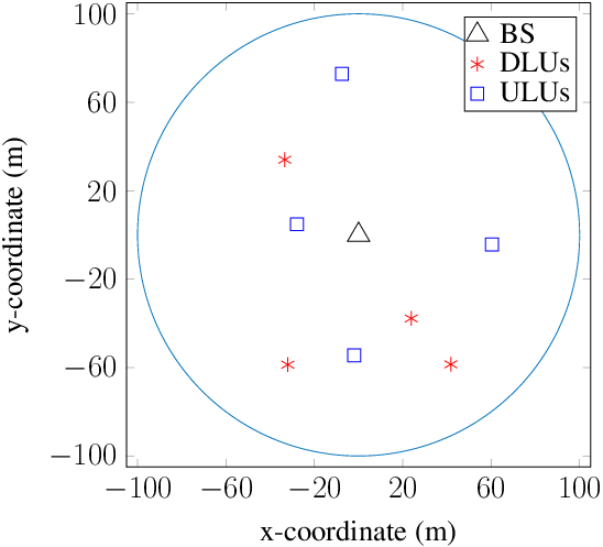

Fig. 4 illustrates the typical convergence behavior of the proposed Algorithms 1 and 2 for the number of groups and different types of power constraints. Both algorithms converge within tens of iterations for all cases. We can see that as increase in the number of groups results in a higher system performance in terms of the SR. In addition, the proposed Algorithm 2 with real power constraints (i.e., (15a) and (16a)) and additional constraints (i.e., (85a) and (86a)) requires 35 iterations, which is the fastest convergence rate when compared to others. Of course, Algorithm 2 using the real power constraints (15a) and (16a) offers better SR compared to that of using the relaxed power constraints (21a) and (22a). Note that the left-hand side (LHS) of (21a) is a sum of power consumptions only, while the LHS of (15a) and (16a) is the total transmit power at the BS. Consequently, by using (21a), the BS and ULUs do not use all allowable power. Thus, the corresponding performance is not optimal. In the following simulation results, we use the power constraints (15a) and (16a) instead of using (21a) and (22a).

In Fig. 5, we depict the effect of the FD residual SI. When the SI is sufficiently canceled dB), the SRs of FD systems are better than those of the HD counterpart by about , , and , corresponding to the proposed FD system with Algorithm 2, Algorithm 1, and the FD system [10], respectively. Generally, the SR of the FD systems is degraded as the residual SI becomes larger dB) and tends to be worse than the HD system for dB. This is probably attributed to the fact that the BS needs to scale down the transmit power in the downlink transmission to avoid a harmful effect on the uplink channel, which results in the SR loss of the FD system. As expected, the FD design with joint optimization of the fraction of time and user grouping assignment in Algorithm 2 offers better SR compared to the fixed design in Algorithm 1 as a result of the optimized transmission. Another interesting observation is that for whatever SI level, the SR of the proposed FD system still outperforms the FD system in [10], and its gain increases when becomes large. The simulation results in Fig. 5 further confirm that the proposed user grouping allows us to exploit the multiuser diversity gain in both channels and also mitigate the effect of the FD residual SI. Due to the advantages of Algorithm 2, from now on, we plot the system performance only with the algorithm.

The SR versus the minimum rate requirement bps/Hz for all users is shown in Fig. 6. This shows that the HD system is fulfilled while the SR of FD design in [10] is degraded dramatically when increases. Notably, the proposed FD design is slightly degraded when becomes higher. In fact, the SR of the system is mostly a contribution of the downlink channel, and thus, the BS must pay more attention to serving ULUs when increases by reducing its transmit power. Recalling the discussion from Fig. 5, the proposed FD design exploits the multiuser diversity gain more efficiently, which in turn improves the user fairness, as shown in Fig. 6. Certainly, the proposed FD system achieves better SR than that of the FD in [10], and the gap between the two is even deeper.

We plot the impact of the number of users on the system performance in Fig. 7. A multiuser system is considered to demonstrate that the proposed FD system can deliver higher SR than conventional FD and HD systems for . The SRs of all designs first increase as and increase up to 8 for a given and then decrease with and because it lacks the degree-of-freedom (DoF) for leveraging multiuser diversity. Of course, the optimal value of and may be different in other settings. For and , the HD system achieves a better SR than the FD system in [10] because of the fact that the BS uses all available antennas () leading to more DoFs available for transmission. Again, the SR of the proposed FD system outperforms that of the others. Thus, the proposed user grouping is a powerful means to combating the DoF bottleneck.
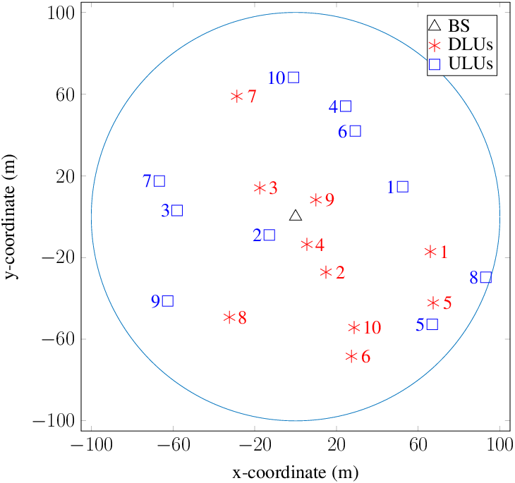
In Fig. 9, we investigate the impact of the number of groups on the system performance for the simulation setup given in Fig. 8. We plot the SR of the proposed FD system versus the minimum rate requirement bps/Hz for = 10. As expected, the SR increases as the number of groups increases, although the gain tends to diminish with . This implies that the larger number of groups would be appropriate for the larger number of users.
Finally, we provide further insight on the proposed FD system by presenting how the users are grouped for the simulation setup given in Fig. 8. There are 20 users in total with 10 DLUs and 10 ULUs for bps/Hz and = 4. The resulting rates in Table II show that the users are divided into different groups. Looking at the , for instance, we can see that its location is very close to the DLUs , , in Fig. 8. Therefore, may cause a large amount of interference to those DLUs. This is the reason why belongs to a group different from such near DLUs, as manifested in Table II. Intuitively, DLUs are served in only one specific group due to reducing the CCI and of course they can be changed in other settings. On the other hand, the FD system in [10] favors the users {, , , } in good channel conditions while barely meeting the rate requirements of the other users. The proposed algorithm is shown to provide better user fairness. Moreover, the proposed FD system yields the SR that is 11.29 bps/Hz higher than the FD system in [10].

| Users | Algorithm 2 () | FD in [10] | |||||
|---|---|---|---|---|---|---|---|
|
|
|
|||||
| DLUs | 1 | 0.500 | 0.000 | 0.000 | 0.500 | 0.500 | |
| 2 | 0.000 | 2.283 | 0.000 | 2.283 | 0.500 | ||
| 3 | 0.000 | 4.042 | 0.000 | 4.042 | 0.500 | ||
| 4 | 0.000 | 0.000 | 1.717 | 1.717 | 0.500 | ||
| 5 | 0.000 | 0.000 | 2.029 | 2.029 | 0.500 | ||
| 6 | 0.687 | 0.000 | 0.000 | 0.687 | 0.500 | ||
| 7 | 0.000 | 0.501 | 0.000 | 0.501 | 0.500 | ||
| 8 | 0.544 | 0.000 | 0.000 | 0.544 | 0.500 | ||
| 9 | 0.000 | 0.000 | 3.154 | 3.154 | 0.500 | ||
| 10 | 1.283 | 0.000 | 0.000 | 1.283 | 0.500 | ||
| ULUs | 1 | 0.695 | 2.407 | 0.570 | 3.672 | 5.116 | |
| 2 | 2.114 | 5.118 | 3.543 | 10.775 | 11.422 | ||
| 3 | 0.668 | 0.714 | 1.295 | 2.677 | 4.490 | ||
| 4 | 0.438 | 0.102 | 0.813 | 1.353 | 0.500 | ||
| 5 | 0.000 | 0.500 | 0.000 | 0.500 | 0.500 | ||
| 6 | 0.000 | 0.248 | 0.252 | 0.500 | 0.500 | ||
| 7 | 0.173 | 0.094 | 1.184 | 1.451 | 0.500 | ||
| 8 | 0.000 | 1.342 | 0.089 | 1.432 | 0.500 | ||
| 9 | 1.083 | 2.899 | 2.197 | 6.179 | 6.201 | ||
| 10 | 0.776 | 1.408 | 1.147 | 3.331 | 2.594 | ||
| Total Sum Rate | |||||||
VI Conclusion
In this paper, we have studied an FD system with joint user grouping, time allocation, beamforming design, and power allocation optimization. To solve the original nonconvex optimization problem, we proposed new iterative algorithms to maximize the total sum rate of the system. The proposed optimization problem captures all important factors in the system performance into low-complexity algorithms. Numerical results with realistic parameters have confirmed that the proposed algorithms are guaranteed to converge to at least the local optima of the original nonconvex design problems. These results have been presented to show a fast convergence rate and to demonstrate the advantages of our proposed algorithms. The sum rate of the proposed FD system has been shown to be remarkably lager than HD if the residual SI is effectively canceled and to always outperform the FD system in [10] with no user grouping in all cases. In addition, the proposed user grouping allows the FD system to exploit the multiuser diversity gain in both directions more efficiently and also to mitigate the effect of the FD residual SI and the CCI.
Appendix: Proof of Proposition 1
Let and denote the objective values of (23a) and (46a), respectively. We have
| (91) |
and
| (92) | |||||
The optimal solutions that are readily seen to return at the -th iteration are also feasible for the considered problem at the -th iteration. Let and be the optimal solutions of (46a) at the -th and at the -th iteration, respectively. It follows that
| (93) | |||||
The inequalities in (93) show that is an improved point to (46a) rather than in the sense of increasing objective value. In addition, the sequence of the objective is bounded above due to the power constraints in (26a) and (27a). By following the same arguments as those in [22, Theorem 1], we can prove that Algorithm 1 converges to a KKT point of (23a). Furthermore, Algorithm 1 will terminate after a finite number of iterations, when it satisfies
where is a given tolerance. Proposition 1 is thus proved.
References
- [1] J. Mietzner, R. Schober, L. Lampe, W. H. Gerstacker, and P. A. Hoeher, “Multiple-antenna techniques for wireless communications -A comprehensive literature survey,” IEEE Commun. Surveys Tutorials, vol. 11, no. 2, pp. 87–105, 2nd Quarter 2009.
- [2] D. Muirhead, M. A. Imran, and K. Arshad, “A survey of the challenges, opportunities and use of multiple antennas in current and future 5G small cell base stations,” IEEE Access, vol. 4, pp. 2952–2964, 2016.
- [3] A. Sabharwal, P. Schniter, D. Guo, D. W. Bliss, S. Rangarajan, and R. Wichman, “In-band full-duplex wireless: Challenges and opportunities,” IEEE J. Select. Areas Commun., vol. 32, no. 9, pp. 1637–1652, Feb. 2014.
- [4] Z. Zhang, X. Chai, K. Long, A. V. Vasilakos, and L. Hanzo, “Full duplex techniques for 5G networks: Self-interference cancellation, protocol design, and relay selection,” IEEE Commun. Magazine, vol. 53, no. 5, pp. 128–137, May 2015.
- [5] “System scenarios and technical requirements for full-duplex concept,” DUPLO project, Deliverable D1.1. [Online]. Available: at http://www.fp7-duplo.eu/index.php/deliverables.
- [6] M. Duarte, C. Dick, and A. Sabharwal, “Experiment-driven characterization of full-duplex wireless systems,” IEEE Trans. Wireless Commun., vol. 11, no. 12, pp. 4296–4307, Dec. 2012.
- [7] E. Everett, A. Sahai, and A. Sabharwal, “Passive self-interference suppression for full-duplex infrastructure nodes,” IEEE Trans. Wireless Commun., vol. 13, no. 2, pp. 680–694, Feb. 2014.
- [8] T. Riihonen, S. Werner, and R. Wichman, “Mitigation of loopback self-interference in full-duplex MIMO relays,” IEEE Trans. Signal Process., vol. 59, no. 12, pp. 5983–5993, Dec. 2011.
- [9] D. Nguyen, L.-N. Tran, P. Pirinen, and M. Latva-aho, “Precoding for full duplex multiuser MIMO systems: Spectral and energy efficiency maximization,” IEEE Trans. Signal Process., vol. 61, no. 16, pp. 4038–4050, Aug. 2013.
- [10] D. Nguyen, L.-N. Tran, P. Pirinen, and M. Latva-aho, “On the spectral efficiency of full-duplex small cell wireless systems,” IEEE Trans. Wireless Commun., vol. 13, no. 9, pp. 4896–4910, Sept. 2014.
- [11] H. H. M. Tam, H. D. Tuan, and D. T. Ngo, “Successive convex quadratic programming for quality-of-service management in full-duplex MU-MIMO multicell networks,” IEEE Trans. Commun., vol. 64, no. 6, pp. 2340–2353, June 2016.
- [12] Y. Li, P. Fan, L. Anatolii, and L. Liu, “On the spectral and energy efficiency of full-duplex small cell wireless systems with massive MIMO,” IEEE Trans. Veh. Technol., to appear, available at http://ieeexplore.ieee.org/stamp/stamp.jsp?arnumber=7486140.
- [13] D. H. N. Nguyen, L. B. Le, and Z. Han, “Optimal uplink and downlink channel assignment in a full-duplex multiuser system,” in Proc. IEEE Inter. Conf. Commun. (ICC 2016), May 2016, pp. 1–6.
- [14] J. M. B. da Silva, G. Fodor, and C. Fischione, “Spectral efficient and fair user pairing for full-duplex communication in cellular networks,” IEEE Trans. Wireless Commun., vol. 15, no. 11, pp. 7578–7593, Nov. 2016.
- [15] M. Ahn, H. B. Kong, H. M. Shin, and I. Lee, “A low complexity user selection algorithm for full-duplex MU-MISO systems,” IEEE Trans. Wireless Commun., vol. 15, no. 11, pp. 7899–7907, Nov. 2016.
- [16] M. Razaviyayn, M. Baligh, A. Callard, and Z. Q. Luo, “Joint user grouping and transceiver design in a MIMO interfering broadcast channel,” IEEE Trans. Signal Process., vol. 62, no. 1, pp. 85–94, Jan. 2014.
- [17] M. Sanjabi, M. Razaviyayn, and Z. Q. Luo, “Optimal joint base station assignment and beamforming for heterogeneous networks,” IEEE Trans. Signal Process., vol. 62, no. 8, pp. 1950–1961, Apr. 2014.
- [18] D. Tse and P. Viswanath, Fundamentals of Wireless Communication. Cambridge Univ. Press, UK, 2005.
- [19] K. Aardal, R. Weismantel, and L. A. Wolsey, “Non-standard approaches to integer programming,” in Discrete Applied Mathematics, pp. 5–74, 2002.
- [20] A. Wiesel, Y. Eldar, and S. Shamai, “Linear precoding via conic optimization for fixed MIMO receivers,” IEEE Trans. Signal Process., vol. 54, no. 1, pp. 161–176, Jan. 2006.
- [21] S. Boyd and L. Vandenberghe, Convex Optimization. Cambridge Univ. Press, UK, 2007.
- [22] B. R. Marks and G. P. Wright, “A general inner approximation algorithm for nonconvex mathematical programs,” Operations Research, vol. 26, no. 4, pp. 681–683, July-Aug. 1978.
- [23] H. Tuy, Convex Analysis and Global Optimization. Kluwer Academic, 2001.
- [24] K. C. Toh, M. J. Todd, and R. H. Tutuncu, “SDPT3-A Matlab software package for semidefinite programming, version 1.3,” Optimization Methods and Softw., vol. 11, pp. 545–581, Jan 1999.
- [25] “I. MOSEK aps,” 2014. [Online]. Available: at http://www.mosek.com.
- [26] A. Ben-Tal and A. Nemirovski, Lectures on Modern Convex Optimization. Philadelphia: MPS-SIAM Series on Optimization, SIAM, 2001.
- [27] 3GPP Technical Specification Group Radio Access Network, Evolved Universal Terrestrial Radio Access (E-UTRA): Further Advancements for E-UTRA Physical Layer Aspects (Release 9), document 3GPP TS 36.814 V9.0.0, 2010.
- [28] D. Bharadia, E. McMilin, and S. Katti, “Full duplex radios,” in Proc. ACM SIGCOMM, 2013.
- [29] J. Lofberg, “YALMIP: A toolbox for modeling and optimization in MATLAB,” in Proc. IEEE Inter. Conf. Robotics and Auto. (IEEE Cat. No.04CH37508), Sept. 2004, pp. 284–289.