Majorana Zero-Modes in a Two-Dimensional $p$-Wave Superconductor

In this section, we derive the projected Hamiltonian describing the two-dimensional $p$-wave topological superconductor used in the main text. A simple four-band model for the valence and conduction bands of the topological insulator Bi₂Se₃ near $\Gamma$ is [30, 31, 50]

where parameters $E_{G},$ $v_{z},$ and $v$ are determined from experimental data. The four bands correspond to the two dominant Wannier orbitals $\{A,B\}$, each with spin $\{\uparrow,\downarrow\}$. The $2\times 2$ Pauli matrices $\sigma_{i}$ and $s_{i}$, with $i=x,y,z,$ act on orbital and spin spaces respectively. We use units where $\hbar=1$, so that all dimensions can be expressed in terms of energies and lengths.

The bands are doubly degenerate with dispersion

The gap between the conduction band and the valence band is thus $2E_{G}$. In order to describe a superconductor, we need to extend the Hilbert space to include hole wavefunctions and a corresponding hole Hamiltonian. Using the convention given in Ref. [50], the full wavefunction now contains eight components,

In this basis, the $8\times 8$ Hamiltonian is simply

where $\epsilon_{F}$ is the Fermi energy, and $\boldsymbol{\tau}$ is a third set of Pauli matrices that couples particles and holes of the same spin and in the same orbital. The particles and holes are now mixed by a triplet, time-reversal-invariant coupling of the form $\Delta=\Delta_{\text{sc}}\sigma_{y}s_{z}\tau_{x}$ that induces a superconducting gap proportional to $\Delta_{\text{sc}}$.

If the energy gap is large, i.e., $2E_{G}\gtrsim\epsilon_{F}-E_{G}$ and $E_{G}\gg\Delta_{\text{sc}}$, only the lower part of the conduction band is occupied and we can neglect the valence band, as the conduction and valence bands are separated by a large energy gap $2E_{G}$. To simplify the result, we first perform a rotation in orbital space by $\pi/2$ about the $y$ axis, so that $\sigma_{y}\rightarrow\sigma_{y},\sigma_{x}\rightarrow\sigma_{z},\sigma_{z}\rightarrow-\sigma_{x}$. In this new representation, the states at the edge of the conduction and valence bands are eigenstates of $\sigma_{z}$, with eigenvalues $\pm 1$. The operators ${\cal P}_{\pm}=({\cal I}\pm\sigma_{z})/2$, where ${\cal I}$ is the identity matrix, thus project the wavefunctions onto the conduction and valence bands respectively. The kinetic energy in Eq. (A1), which is now proportional to $\sigma_{x}$, and the gap, which remains proportional to $\sigma_{y}$, mix the conduction and valence bands. Using perturbation theory, we can expand the Hamiltonian to first order in $\Delta_{\text{sc}}$ and then project onto the conduction band to find the reduced Hamiltonian

Using $\sigma_{z}^{-1}=\sigma_{z},\tau_{z}^{-1}=\tau_{z}$, and adding the chemical potential that was omitted in Eq. (A5), we obtain

where $\bar{\epsilon}_{F}=\epsilon_{F}-E_{G}$.

This Hamiltonian defines a three-dimensional topological superconductor. The Fermi wave-vector and the coherence length along to the $z$-direction are given by

We now analyze a quasi-two-dimensional system of thickness $d$, where $k_{Fz}^{-1}\ll d\lesssim\xi_{z}$. In the absence of superconductivity, the Hamiltonian can be separated as ${\cal H}^{\text{red}}={\cal H}_{\parallel}+{\cal H}_{z}$, where ${\cal H}_{\parallel}$ and ${\cal H}_{z}$ are the in-plane and out-of-plane components of the Hamiltonian, respectively. The electronic states can then be divided into sub-bands, $\epsilon_{n}({\bf k})=\epsilon_{z}^{n}+\epsilon_{\parallel}({\bf k})$. Here, $\epsilon_{z}^{n}$ and $\epsilon_{\parallel}({\bf k})$ are eigenvalues of ${\cal H}_{z}$ and ${\cal H}_{\parallel}$, respectively, and $\mathbf{k}$ is the two-dimensional wave-vector in the $x$-$y$ plane. The separation of levels due to the quantization in the $z$-direction is, approximately,

where $\Delta_{\text{exp}}$ is the value of the measured superconducting gap at the Fermi energy, see Eq. (A6). In order to define a low-energy effective theory for the electronic structure, we study first the lowest energy state for $|{\bf k}|\approx 0$ and energy $|\epsilon|\sim\Delta_{\text{sc}}\ll\delta\epsilon_{z}^{n}$.

For $|{\bf k}|=0$, the Hamiltonian in Eq. (A6) can be split into two $2\times 2$ Hamiltonians, one which mixes electrons and holes with spin up, and another one which mixes electrons and holes with spin down. The two Hamiltonians are related by time-reversal symmetry. For $d\gtrsim\xi_{z}$ the lowest states of these Hamiltonians are localized at the top and bottom surfaces. The decay length of these states is given by the coherence length $\xi_{z}$. When $d\lesssim\xi_{z}$, these states hybridize, and give rise to two Andreev states at energies $\pm\epsilon_{0}\lesssim\Delta_{\text{sc}}$. Thus, the combination of the two $2\times 2$ Hamiltonians gives rise to four low-energy states, $|i\rangle,i=1,\cdots,4$, related by particle-hole and time-reversal symmetries.

A generic wavefunction in this low-energy sector can be written as $\sum_{i}\psi_{i}(\mathbf{r})|i\rangle$, where $\mathbf{r}$ is a two dimensional vector. Using the basis of states $|i\rangle$, we can write an effective Hamiltonian whose states are four-component spinors. Without loss of generality, we can label the two states at energy $+\epsilon_{0}$ as $|e\uparrow\rangle$ and $|e\downarrow\rangle$, and the two spinors with energy $-\epsilon_{0}$ as $|h\uparrow\rangle$ and $|h\downarrow\rangle$. We assume that the matrix elements of the spin Pauli matrices $s_{i}$ and the electron-hole Pauli matrices $\tau_{i}$ ($i=x,y,z$) have the same values in this basis as in the original basis of spins and electron-hole states. Hence, we can write the effective Hamiltonian for the in-plane wavefunction in terms of $x$ and $y$ coordinates as

This Hamiltonian can be split into two independent Hamiltonians related by time-reversal symmetry. These Hamiltonians mix electrons with spin up and holes with spin down, and vice versa.

We make an approximate decomposition into a state with small $|\mathbf{k}|$, and a lowest energy $k_{z}$ state. To good approximation, the Hamiltonian depends only on $k_{z}$,

A standard plane-wave solution to this Hamiltonian has eigenvalues

This spectrum has an energy gap of about $4/\xi_{z}k_{Fz}$ due to superconductivity.

We can solve for the eigenenergies; values of the parameter $\epsilon_{0}$ in Eq. (A9) are shown in Fig. A1 for a realistic choice of parameters. Here we require that the superconducting gap is 0.6 meV. For energy eigenvalues inside the gap, $\epsilon_{0}/\bar{\epsilon}_{F}<2/\xi_{z}k_{Fz},$ we have states that are weakly localized at the top and bottom surfaces, with an exponential decay slower than the thickness of the disc. As illustrated in Fig. A1, there is a wide range of values for $d$ for which we find a state inside or near the gap.

We note that for $k_{Fz}^{-1}=20\penalty\ \mathrm{\AA}$, we have $\xi_{z}=4000\penalty\ \mathrm{\AA}$ (a smaller Fermi wavevector leads to an even larger coherence length for a fixed gap). This shows that our system needs not be atomistically thin, but can have a thickness on the order of a thousand angstroms, similar to the coherence length. Henceforth, without loss of generality, we assume we have chosen a particular thickness $d$ for the disc where no localization at the surfaces occurs. We also absorb $\epsilon_{0}$ into the definition of $\bar{\epsilon}_{F}$. This does not change the value of $\bar{\epsilon}_{F}$ appreciably because $\bar{\epsilon}_{F}$ is much larger than $\epsilon_{0}.$

The two reduced Hamiltonians can be interpreted as describing two metals with quadratic dispersion and superconducting gaps at the Fermi surface with angular dependence $\Delta_{\text{sc}}^{\text{Fermi}}=2v_{F}k_{F}\Delta_{\text{sc}}e^{i\varphi}/E_{G}$, where $\varphi=\arctan(k_{y}/k_{x})$ is the angular coordinate in momentum space, and $k_{F}=\sqrt{2E_{G}\bar{\epsilon}_{F}/v_{F}^{2}}$. In experiments, the more relevant energy scale is the superconducting energy gap measured at the Fermi surface $2\Delta_{\text{exp}}=2|\Delta_{\text{sc}}^{\text{Fermi}}|=4v_{F}k_{F}\Delta_{\text{sc}}/E_{G}.$ The two Hamiltonians are

The two Hamiltonians are related by time inversion. Each Hamiltonian describes a chiral $p$-wave superconductor [14]. The energy dispersion is

Using the convention where

the full Hamiltonian should be written as

where

and ${\cal H}_{-}(\mathbf{k})=-{\cal H}_{+}(-\mathbf{k})$.

In this section, we solve for the edge modes on a disc. As noted above, the low-energy states in the conduction band of the two-dimensional superconductor doped Bi₂Se₃ can be described by two effective $p$-wave Hamiltonians that couple electrons and holes of opposite spins defined by Eqs. (A16) and (A). The $p^{+}$ and $p^{-}$ superconducting branches are related by time-reversal symmetry. Thus, since eigenstates of $\mathcal{H}_{+}$ are also eigenstates of $\mathcal{H}_{-}$, we restrict our attention to $\mathcal{H}_{+}$ on a circle of radius $R$. In polar coordinates, we have $\pm ik_{x}+k_{y}=\pm e^{\pm i\theta}\left(\partial_{r}\mp i\partial_{\theta}/r\right)$, and $k_{x}^{2}+k_{y}^{2}=-\nabla^{2}=-\partial_{r}^{2}-\partial_{r}/r-\partial^{2}_{\theta}/r^{2}$. Using separation of variables, we can write our wavefunction in coordinate space as

To insist that the wavefunction is single-valued, we have that $\ell$ must be an integer. In this case, $\ell$ takes the role of describing our angular momentum quantum number. Let us now show that indeed, $\ell$ can be used as a good quantum number. The angular momentum operator in this case is

where $\mathcal{I}$ is the identity matrix. The spectrum of $L_{z}$ is $L_{z}\Psi_{\ell}=\left(\ell+\frac{1}{2}\right)\Psi_{\ell}$. By using the fact that partial derivatives commute, it immediately follows that $[\mathcal{H}_{+},L_{z}]=0$. Consequently, we can diagonalize both $\mathcal{H}_{+}$ and $L_{z}$ simultaneously, and use $\ell$ as a good quantum number.

Using the form of $\Psi$ in Eq. (A19), we find that the radial wavefunctions satisfy the following eigenvalue problem

To solve for the radial wavefunction, we make an ansatz that the wavefunction components are Bessel functions based on the motivation that eigenfunctions of the Laplacian are Bessel functions

where $a$ and $b$ are constants, $J_{\ell}(x)$ is the Bessel function of the first kind of order $\ell,$ and $k$ is the linear momentum in the radial direction. Substituting this ansatz into Eq. (A21), our problem is reduced to a simple eigenvalue problem

This has unnormalized solutions

where

Having found the eigenstates of our topological superconductor, we can now study the effect of the edge. We impose hard-wall boundary condition whereby we require the wavefunction to vanish at the perimeter of the disc $\Psi_{\ell}(R,\theta)=0$. This condition is equivalent to continuity of the Dirac wavefunction at the boundary where we have Andreev reflections [34]. In order to satisfy this condition, the wavefunction for a particular energy $E$ must be a linear combination of outgoing and reflected waves.

Let us now simplify by using dimensionless variables, where we express lengths in terms of the Fermi momentum $k_{F}=\sqrt{2E_{G}\bar{\epsilon}_{F}}/v_{F}$ as defined in the main text, and all energies in terms of $\bar{\epsilon}_{F}$,

where $\gamma=\frac{4\Delta_{\text{sc}}^{2}}{E_{G}\bar{\epsilon}_{F}}=\frac{\Delta_{\text{exp}}^{2}}{2\bar{\epsilon}_{F}^{2}}\ll 1$ measures the superconducting gap relative to $E_{G}$ and $\bar{\epsilon}_{F}$ and $\mathcal{E}=E/\bar{\epsilon}_{F}$. In terms of these parameters, the full wavefunction is

where $\rho=r/R$ is the fractional radius, and $\lambda=k_{F}R$ is the dimensionless system size. Setting both components of the above equation to zero at $\rho=1$, we obtain the following transcendental equation for the allowed energies

We can numerically solve this transcendental equation for some typical parameter values, given that we stay within the regime of validity for our effective Hamiltonian. To obtain an edge state with energy below the gap, we can consider the limit of a very large disc, as done in [34]. Suppose that $\lambda\gg 1$, then for a very small angle $\theta\ll 1$, the boundary resembles that of the infinite half plane for which we know that the edge state has energy $\mathcal{E}^{\text{edge}}=-\frac{2v_{F}k_{x}\Delta_{\text{sc}}}{E_{G}\bar{\epsilon}_{F}}$, where $k_{x}$ is the linear momentum along the edge [34, 15]. Translating this result to our geometry in the semi-classical limit, we have $|\mathbf{L}|=|\mathbf{r}\times\mathbf{p}|=\ell\approx Rk_{x}.$ Thus, approximately, the energy of the edge state in the semi-classical limit is $\mathcal{E}_{\text{edge}}\approx-\frac{\ell}{\ell_{0}}\delta$, where $\delta=\Delta_{\text{sc}}/\bar{\epsilon}_{F}$ and $\ell_{0}=RE_{G}/2v_{F}$. We can tighten this estimate further using a general argument of particle-hole symmetry; that is, if $\mathcal{H}\Psi=E\Psi$, then $\mathcal{H}(\tau_{x}\mathcal{C}\Psi)=-E(\tau_{x}\mathcal{C}\Psi),$ where $\mathcal{C}$ is the complex-conjugation operator. With this, we see that a state of angular momentum $\ell$ has the opposite energy to a state of angular momentum $-(\ell+1)$. Therefore, we find that the edge energy is

This can be further improved by a more detailed asymptotic analysis. We find

with a numerical indication that the next order has a more complex dependence on $\ell$.

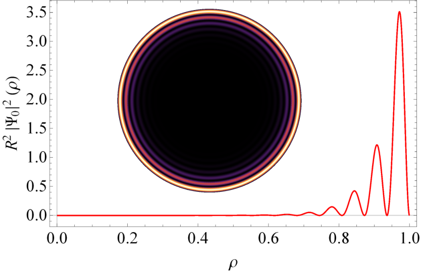
We compare in Fig. A2 the functional form of Eq. (A29) to the lowest energy found from the transcendental equation in Eq. (A28). To leading order in $\lambda^{-1}$, there is good agreement between the numerical result and the approximation in Eq. (A29). This energy spectrum lies inside the superconducting gap, and corresponds to edge states at the perimeter of the disc. One such edge state for $\ell=0$ is shown in Fig. A3. The edge mode we have found is the chiral edge state we have sought from the beginning. From Eq. (A29) we see that each of the Hamiltonians $\mathcal{H}_{\pm}$ describes a single chiral band with unidirectional group velocity—negative for the case described here. This reflects the fact that a single chiral Hamiltonian breaks time-reversal invariance.

To recover time-reversal invariance, we now consider the full Hamiltonian, Eq. (A16), of the two-dimensional topological superconductor. The spectrum of edge modes for $\mathcal{H}_{-}$ consists of the time-reversed states of $\mathcal{H}_{+}$. Suppose a state $\Psi_{+}^{\text{edge}}$ is an eigenstate of $\mathcal{H}_{+}$ of angular momentum $\ell$, then the time-reversed state with angular momentum $-(\ell+1)$ is an eigenstate of $\mathcal{H}_{-}$. Therefore, the edge spectrum of $\mathcal{H}_{-}$ is

This is just the chiral spectrum for modes propagating in the other direction. Taken together, Eqs. A29 and A31 give the full spectrum of the two edge modes for our time-reversal-invariant topological superconductor. The band structure of this system is shown in Fig. A2.

In this section, we consider the effect of a constant in-plane Zeeman field defined by

where $\mathcal{E}_{Z}$ is the energy magnitude of the field, $\mathbf{n}$ is a unit normal along the direction of the field, and $\phi$ is the angle of that field. This Zeeman field couples electrons of opposite spins and holes of opposite spins, both with the same sign. By construction, this addition to the Hamiltonian explicitly breaks time-reversal symmetry. The full Hamiltonian now becomes

where $\mathcal{H}_{0}$ is defined by Eq. (A16). We consider $\mathcal{H}_{Z}$ as a weak perturbation to $\mathcal{H}_{0}$, in comparison to the low-lying edge states with energies below the superconducting gap. That is, we assume $\mathcal{E}_{Z}\ll\delta$. So we can use lowest-order perturbation theory to assess how the energy spectrum of the low-lying edge states is changed. We first write explicitly the full edge wavefunctions. With $C_{+}$ and $C_{-}$ in Eq. (A27) related by the vanishing boundary condition

we can write the wavefunction in the $\mathcal{H}_{+}$ subspace as

where $\mathcal{N}$ is a normalization constant. We can simplify the wavefunction further by noting that

where the last equality follows from inspection of Eq. (A26) that for $\mathcal{E}<\delta$, $\kappa_{\pm}$ is complex, and consequently, $\kappa_{+}^{*}=\kappa_{-}$. Using this, it is clear that the radial part of Eq. (A35) is purely imaginary