Numerical algorithms for mean exit time and escape probability of stochastic systems with asymmetric Lévy motion

Xiao Wang Affiliation: School of Mathematics and Statistics, Henan UniversityKaifeng 475001, Chinaemail xiaoheda06@163.com Jinqiao Duan Affiliation: Department of Applied Mathematics, Illinois Institute of TechnologyChicago, IL 60616, USA email duan@iit.edu(J. Duan), lix@iit.edu(X. Li) Xiaofan Li Note: Corresponding author. Affiliation: Department of Applied Mathematics, Illinois Institute of TechnologyChicago, IL 60616, USA email duan@iit.edu(J. Duan), lix@iit.edu(X. Li) Renming Song Affiliation: Department of Mathematics, University of IllinoisUrbana, IL 61801, USAemail rsong@math.uiuc.edu

Abstract

For non-Gaussian stochastic dynamical systems, mean exit time and escape probability are important deterministic quantities, which can be obtained from integro-differential (nonlocal) equations. We develop an efficient and convergent numerical method for the mean first exit time and escape probability for stochastic systems with an asymmetric Lévy motion, and analyze the properties of the solutions of the nonlocal equations. We also investigate the effects of different system factors on the mean exit time and escape probability, including the skewness parameter, the size of the domain, the drift term and the intensity of Gaussian and non-Gaussian noises. We find that the behavior of the mean exit time and the escape probability has dramatic difference at the boundary of the domain when the index of stability crosses the critical value of one.

Key words: Stochastic dynamical systems Asymmetric Lévy motion Integro-differential equation First exit time Escape probability

1 Introduction

Non-Gaussian stochastic dynamical systems are found in many applications such as economics, telecommunications and physics [19, 12, 13]. As a special non-Gaussian stochastic process, $\alpha$ -stable Lévy process (or often called $\alpha$ -stable Lévy motion) attracts more and more attentions of mathematicians due to the properties which the Gaussian process does not have. For example, the tail of a Gaussian random variable decays exponentially which does not fit well for modeling processes with high variability or some extreme events, such as earthquakes or stock market crashes. However, the stable Lévy motion has a ‘heavy tail’ that decays polynomially and could be useful for these applications. For example, financial asset returns could present heavier tails relative to the normal distribution, and asymmetric $\alpha$ -stable distributions are proper alternatives for modeling them [17]. Others considered the applications in financial risks, physics, and biology [20, 7, 9].

Recently, many researchers begin to pay attention to the stochastic dynamical systems with asymmetric stable Lévy motion due to the demand from applications [2, 30, 7]. For instance, Lambert [14] considers the first passage time and leapovers with an asymmetric stable Lévy motion.

In this present work, we consider the following scalar stochastic differential equation (SDE)

\displaystyle{\rm d}X_{t}=f(X_{t}){\rm d}t+{\rm d}L_{t},

(1.1)

where the initial condition is $X_{0}=x$ , $f$ is a drift term (vector field), and $L_{t}$ is a Lévy process with the generating triplet $(0,d,\epsilon\nu_{\alpha,\beta})$ (when $d$ is taken zero, it is just an asymmetric stable Lévy motion). Here, $\nu_{\alpha,\beta}$ is an asymmetric Lévy jump measure on $\mathbb{R}\setminus\{0\}$ , to be specified in the next section. The well-posedness of SDE driven by Lévy motion is discussed recently. The existence and uniqueness of solutions under the standard Lipschitz and growth conditions driven by Brownian motion and independent Poisson random measure were given, for example, Applebaum [1] . Lü et al.[16] obtained a unique solution for stochastic quasi-linear heat equation driven by anisotropic fractional Lévy noises under Lipschtz and linear conditions. Chen et al.[4] showed the SDE with a large class of Lévy process had a unique strong solution for Hölder continuous drift $f$ . Priola et al.[22] showed the pathwise uniqueness for SDE driven by nondegenerate symmetric $\alpha$ -stable Lévy process. We focus on the macroscopic behaviors, particularly the mean exit time and escape probability, for the SDE (1.1) with an asymmetric stable Lévy motion.

There are numerous works discussing the symmetric $\alpha$ -stable Lévy motion and the corresponding infinitesimal generator, which is a nonlocal operator and is also called the fractional Laplacian operator $(-\triangle)^{\frac{\alpha}{2}}$ . It is equivalent to fractional derivative as follows,

(-\triangle)^{\frac{\alpha}{2}}u(x)=\frac{{}_{-L}D_{x}^{\alpha}u(x)+{}_{x}D_{L}^{\alpha}u(x)}{2\cos{\frac{\pi\alpha}{2}}}\quad\text{ for }\alpha\neq 1,

where ${}_{-L}D_{x}^{\alpha}u(x)$ and ${}_{x}D_{L}^{\alpha}u(x)$ are left and right Riemann-Liouville fractional derivatives [11, 31]. Various numerical methods are developed for the fractional Laplacian and the fractional derivative operators. To name a few, Li et al. [15] considered the spectral approximations to compute the fractional integral and the Caputo derivative. Mao et al. [18] developed an efficient Spectral-Galerkin algorithms to solve fractional partial differential equations(FPDEs). Du et al. [5] considered the general nonlocal integral operator and provide guidance for numerical simulations. Qiao et al. [23] used asymptotic methods to examine escape probabilities analytically. Gao et al. [8] developed a finite difference method to compute mean exit time and escape probability in the one-dimensional case. Our previous work [29] proposed a method to compute the mean exit time and escape probability for two-dimensional stochastic systems with rotationally symmetric $\alpha$ -stable type Lévy motions.

For stochastic systems with the asymmetric Lévy motion, research on macroscopic quantities, such as mean exit time and escape probability, is still at its initial stage. A couple of papers [14, 2] considered the exit problem of the completely asymmetric Lévy motion (corresponding to $\beta=1$ or $-1$ in the jump measure $\nu_{\alpha,\beta}$ ). A few of people have studied the processes for their basic properties. Considering a completely asymmetric Lévy process that has absolutely continuous transition probabilities, Bertoin [3] proved the decay and ergodic properties of the transition probabilities while Lambert [14] established the existence of the Lévy process conditioned to stay in a finite interval. Koren et al. [13] investigated the first passage times and the first passage leapovers of symmetric and completely asymmetric Lévy stable random motions.

The paper is organized as follows. In Section 2, we review the concepts of asymmetric Lévy motion, mean exit time and escape probability, and show the symmetry of solutions to the exit problem. A numerical method and simulation results for mean exit time and escape probability are presented in Section 3 and 4, respectively. Finally, Section 5 presents the conclusion of our paper.

2 Concepts

2.1 Asymmetric Lévy motion

Stable distribution, denoted by $S_{\alpha}(\sigma,\beta,\mu)$ , is a four-parameter family of distributions with $\alpha\in(0,2],\sigma\geq 0,\beta\in[-1,1]$ and $\mu\in{\mathbb{R}}$ . Usually $\alpha$ is called the index of stability (or non-Gaussianity index), $\sigma$ is the scale parameter, $\beta$ is the skewness parameter and $\mu$ is the shift parameter. It is said to be completely asymmetric if $\beta=\pm 1$ [26, 27, 1]. Stable distribution and its profile help us understand the behavior of the process governed by the SDE (1.1), because $L_{1}$ is a random variable with the probability density functions(PDFs) of $S_{\alpha}(1,\beta,0)$ . The corresponding generating triplet is $(K_{\alpha,\beta},0,\nu_{\alpha,\beta})$ , where the constant $K_{\alpha,\beta}$ and the jump measure $\nu_{\alpha,\beta}$ are defined below in (2.7) and (2.4) respectively. Some examples of $S_{\alpha}(1,\beta,0)$ are shown in Figure 1.

Refer to caption — Figure 1: Probability density functions $S_{\alpha}(1,\beta,0)$ of $L_{1}$ for different values of $\alpha$ and $\beta$ .

For the $\alpha$ -stable Lévy motion, we have the corresponding Lévy-Khinchin formula [27, 21, 10]

\displaystyle\mathbb{E}(e^{i\lambda L_{t}})=\begin{cases}\mbox{exp}\{-\sigma^{\alpha}|\lambda|^{\alpha}t(1-i\beta\mbox{sgn}{\lambda}\tan{\frac{\pi\alpha}{2}})+i\mu\lambda t\},\;\mbox{for}\;\alpha\neq 1,\\ \mbox{exp}\{-\sigma|\lambda|t(1+i\beta\frac{2}{\pi}\mbox{sgn}{\lambda}\log{|\lambda|})+i\mu\lambda t\},\quad\mbox{for}\;\alpha=1.\end{cases}

(2.2)

For every $\varphi\in H_{0}^{2}({\mathbb{R}})$ , we can obtain the generator for the solution to the SDE (1.1) with the asymmetric $\alpha$ -stable Lévy motion $L_{t}$ from the above formula (2.2) as [27, 6]

	$\displaystyle\mathscr{L}\varphi(x)=$	$\displaystyle(f(x)+\epsilon K_{\alpha,\beta})\varphi^{\prime}(x)+\frac{d}{2}\varphi^{\prime\prime}(x)$
		$\displaystyle+\epsilon\int_{\mathbb{R}\setminus\{0\}}\left(\varphi(x+y)-\varphi(x)-1_{B}\;y\varphi^{\prime}(x)\right)\nu_{\alpha,\beta}({\rm d}y),$		(2.3)

where the measure $\nu_{\alpha,\beta}$ is given by

\displaystyle\nu_{\alpha,\beta}({\rm d}y)=\frac{C_{1}1_{\{0<y<\infty\}}(y)+C_{2}1_{\{-\infty<y<0\}}(y)}{|y|^{1+\alpha}}({\rm d}y)

(2.4)

with

\displaystyle C_{1}=C_{\alpha}\frac{1+\beta}{2},C_{2}=C_{\alpha}\frac{1-\beta}{2},\quad-1\leq\beta\leq 1,

(2.5)

and

\displaystyle C_{\alpha}=\begin{cases}\frac{\alpha(1-\alpha)}{\Gamma(2-\alpha)\cos{(\frac{\pi\alpha}{2})}}\;,&\text{ $\alpha\neq 1$;}\\ \frac{2}{\pi},\;&\text{ $\alpha=1$.}\end{cases}

(2.6)

In Eq. (2.3) the constants $d$ and $\epsilon$ represent the intensities of Gaussian and Lévy noises respectively.

The constant $K_{\alpha,\beta}$ in (2.3) is given by

\displaystyle K_{\alpha,\beta}=\begin{cases}\frac{C_{1}-C_{2}}{1-\alpha}\;,&\text{ $\alpha\neq 1$;}\\ (\int_{1}^{\infty}\frac{\sin(x)}{x^{2}}{\rm d}x+\int_{0}^{1}\frac{\sin(x)-x}{x^{2}}{\rm d}x)(C_{2}-C_{1}),\;&\text{ $\alpha=1$.}\end{cases}

(2.7)

Furthermore, we note that $\beta=\frac{C_{1}-C_{2}}{C_{1}+C_{2}}$ , and the symmetries $C_{1}(-\beta)=C_{2}(\beta)$ and $K_{\alpha,-\beta}=-K_{\alpha,\beta}$ . We point out that when $\alpha\neq 1$ the stable distribution is strictly $\alpha$ -stable, while it is strictly $\alpha$ -stable when $\alpha=1$ if and only if its Lévy measure is symmetric.

We remark that, for people who are not too familiar with stable distributions, the non-solid curves in Fig. 1(b) and (c) might be counter intuitive. After all, in both figures, the skewness parameter $\beta$ is positive in all these case and thus there is a bigger tendency of jumping to the right, and yet these curves are shifted to left near the origin. This is due to the compensation which produces a linear drift with coefficient $K_{\alpha,\beta}$ given by (2.7). In all these cases, $K_{\alpha,\beta}$ is negative.

2.2 Mean exit time and escape probability

The exit time problem is important in many fields, such as physiscs, finance and economics. The first exit time starting at $x$ from a bounded domain $D$ is defined as $\tau{(\omega)}:=\inf\{t\geq 0,X_{t}(\omega,x)\notin D\}$ , and the mean first exit time (MET) is $u(x)=\mathbb{E}[\tau(\omega)].$

Assume that $f(x)$ satisfies Lipschitz condition and linear growth condition for the existence and uniqueness of solution [1]. Due to the Dynkin’s formula, the MET $u$ satisfies the following nonlocal partial differential equation [6]

\displaystyle\mathscr{L}u(x)

\displaystyle=-1,\quad\text{for}\;x\in D,

(2.8)

subject to the Dirichlet-type exterior condition,

\displaystyle u(x)

\displaystyle=0,\quad\text{for}\;x\in D^{c},

(2.9)

where $\mathscr{L}$ is the generator defined in (2.3) and $D$ is open.

Consider the escape probability of the process $X_{t}$ in the SDE (1.1). The escape probability from $D$ to $E$ is the likelihood that $X_{t}$ with the initial location $X_{0}=x$ , exits from $D$ and first lands in $E$ which belong to $D^{c}$ , denoted as $P_{E}(x)=\mathbb{P}\{X_{\tau}\in E\}$ . The escape probability satisfies the following nonlocal partial differential equation [24, 6]

	$\displaystyle\mathscr{L}\,P_{E}(x)=0,\quad x\in D,$
	$\displaystyle P_{E}\|_{x\in E}=1,\quad P_{E}\|_{x\in D^{c}\setminus E}=0.$		(2.10)

2.3 Symmetry and non-dimensionalization

For the domain $D=(-b,b)$ , the MET $u$ satisfies Eq. (2.8). We replace the $I_{\{|y|<1\}}(y)$ in Eq. (2.8) to $I_{\{|y|<b\}}(y)$ and get [27]

	$\displaystyle\frac{d}{2}u^{\prime\prime}(x)+c(x)u^{\prime}(x)+\varepsilon\int_{{\mathbb{R}}\setminus\{0\}}[u(x+y)-u(x)-I_{\{\|y\|<b\}}(y)\;yu^{\prime}(x)]$		(2.11)
	$\displaystyle\left[\frac{C_{1}1_{\{0<y<\infty\}}+C_{2}1_{\{-\infty<y<0\}}}{\|y\|^{1+\alpha}}\right]\;{\rm d}y=-1,$

where

\displaystyle c(x)=\begin{cases}f(x)+\epsilon K_{\alpha,\beta}+\varepsilon(C_{1}-C_{2})\frac{b^{1-\alpha}-1}{1-\alpha}\;,&\text{ $\alpha\neq 1$;}\\ f(x)+\epsilon K_{\alpha,\beta}+\varepsilon(C_{1}-C_{2})\ln{b},\;&\text{ $\alpha=1$.}\end{cases}

(2.12)

Next, we show the solution to the MET problem has the following symmetry when $f$ is an odd function. However, the numerical method presented in the work does not require $f$ be odd. Because of the application in dynamical systems, we focus on the O-U potential( $f(x)=-x$ ) later.

Proposition 2.1 (Symmetry of Solutions).

If $f(x)$ is an odd function and the domain $D$ is symmetric about the origin ( $D=(-b,b)$ ), then the MET $u$ (or, equivalently, the solution $u$ to Eq. (2.11)) is symmetric about the origin if $\beta$ changes the sign, i.e. $u_{-\beta}(-x)=u_{\beta}(x)$ for all $x\in(-b,b)$ where $u_{\beta}$ and $u_{-\beta}$ denote the solutions corresponding to $\beta$ and $-\beta$ respectively.

Proof.

Since Eq. (2.11) is valid for all $-1\leqslant\beta\leqslant 1$ and $-b\leqslant x\leqslant b$ , $u_{-\beta}(-x)$ satisfies the following equation,

			$\displaystyle\frac{d}{2}u_{-\beta}^{\prime\prime}(-x)+c(-x)u_{-\beta}^{\prime}(-x)$
	$\displaystyle+$		$\displaystyle\varepsilon\int_{{\mathbb{R}}\setminus\{0\}}[u_{-\beta}(-x+y)-u_{-\beta}(-x)-I_{\{\|y\|<b\}}(y)\;yu_{-\beta}^{\prime}(-x)]\nu_{\alpha,-\beta}({\rm d}y)=-1.$

Define $\bar{u}(x)=u_{-\beta}(-x)$ . We can see $\bar{u}^{\prime}(x)=-u_{-\beta}^{\prime}(-x)$ . Taking $y^{\prime}=-y$ , we have

			$\displaystyle\int_{{\mathbb{R}}\setminus\{0\}}[u_{-\beta}(-x+y)-u_{-\beta}(-x)-I_{\{\|y\|<b\}}(y)\;yu_{-\beta}^{\prime}(-x)]\nu_{\alpha,-\beta}({\rm d}y)$
		$\displaystyle=$	$\displaystyle\int_{{\mathbb{R}}\setminus\{0\}}[\bar{u}(x-y)-\bar{u}(x)+I_{\{\|y\|<b\}}(y)\;y\bar{u}^{\prime}(x)]\left[\frac{C_{2}1_{\{0<y<\infty\}}+C_{1}1_{\{-\infty<y<0\}}}{\|y\|^{1+\alpha}}\right]\;{\rm d}y$
		$\displaystyle=$	$\displaystyle\int_{{\mathbb{R}}\setminus\{0\}}[\bar{u}(x+y^{\prime})-\bar{u}(x)-I_{\{\|y^{\prime}\|<b\}}(y^{\prime})\;y^{\prime}\bar{u}^{\prime}(x)]\left[\frac{C_{1}1_{\{0<y^{\prime}<\infty\}}+C_{2}1_{\{-\infty<y^{\prime}<0\}}}{\|y^{\prime}\|^{1+\alpha}}\right]\;{\rm d}y^{\prime}.$

When $f(-x)=-f(x)$ , we have

\displaystyle c(-x)=\begin{cases}-f(x)+\epsilon K_{\alpha,\beta}+\varepsilon C_{\alpha}\beta\frac{b^{1-\alpha}-1}{1-\alpha}\;,&\text{ $\alpha\neq 1$;}\\ -f(x)+\epsilon K_{\alpha,\beta}+\varepsilon C_{\alpha}\beta\ln{b},\;&\text{ $\alpha=1$.}\end{cases}

Thus $c_{-\beta}(-x)=-c_{\beta}(x)$ if $f$ is an odd function, where $c_{\beta}$ and $c_{-\beta}$ denote the function $c$ corresponding to $\beta$ and $-\beta$ respectively.

Using

\frac{d}{2}u_{-\beta}^{\prime\prime}(-x)+c_{-\beta}(-x)u_{-\beta}^{\prime}(-x)=\frac{d}{2}\bar{u}^{\prime\prime}(x)+c_{\beta}(x)\bar{u}^{\prime}(x),

we get,

	$\displaystyle\frac{d}{2}\bar{u}^{\prime\prime}(x)+c(x)\bar{u}^{\prime}(x)+\varepsilon\int_{{\mathbb{R}}\setminus\{0\}}[\bar{u}(x+y^{\prime})-\bar{u}(x)-I_{\{\|y^{\prime}\|<b\}}(y^{\prime})\;y^{\prime}\bar{u}^{\prime}(x)]$
	$\displaystyle\left[\frac{C_{1}1_{\{0<y^{\prime}<\infty\}}+C_{2}1_{\{-\infty<y^{\prime}<0\}}}{\|y^{\prime}\|^{1+\alpha}}\right]\;{\rm d}y^{\prime}=-1.$

Thus, we have shown $\bar{u}(x)$ satisfies the same Eq. (2.11) if $f(-x)=-f(x)$ . Due to uniqueness of the solution, we have $u_{-\beta}(-x)=u_{\beta}(x)$ . $\Box$ ∎

To keep the computational domain fixed as $[-1,1]$ , we perform the change of variable

s=x/b,\quad\text{ and }v(s):=u(bs).

(2.13)

Then, $\displaystyle{\frac{{\rm d}u}{{\rm d}x}=\frac{1}{b}\frac{{\rm d}v}{{\rm d}s},\;\frac{{\rm d}^{2}u}{{\rm d}x^{2}}=\frac{1}{b^{2}}\frac{{\rm d}^{2}v}{{\rm d}s^{2}}}$ . Let $y=br$ , we have

			$\displaystyle\int_{{\mathbb{R}}\setminus\{0\}}[u(x+y)-u(x)-I_{\{\|y\|<b\}}(y)\;yu^{\prime}(x)]\left[\frac{C_{1}1_{\{0<y<\infty\}}+C_{2}1_{\{-\infty<y<0\}}}{\|y\|^{1+\alpha}}\right]\;{\rm d}y$
		$\displaystyle=$	$\displaystyle b^{-\alpha}\int_{{\mathbb{R}}\setminus\{0\}}[v(s+r)-v(s)-I_{\{\|r\|<1\}}(r)\;rv^{\prime}(s)]\left[\frac{C_{1}1_{\{0<r<\infty\}}+C_{2}1_{\{-\infty<r<0\}}}{\|r\|^{1+\alpha}}\right]{\rm d}r$

Finally, the equation for the MET (2.11) becomes

	$\displaystyle\frac{d}{2b^{2}}\frac{{\rm d}^{2}v}{{\rm d}s^{2}}+\frac{c(bs)}{b}\frac{{\rm d}v}{{\rm d}s}$	(2.14)
$\displaystyle+$	$\displaystyle\varepsilon b^{-\alpha}\int_{{\mathbb{R}}\setminus\{0\}}[v(s+r)-v(s)-I_{\{\|r\|<1\}}(r)\;rv^{\prime}(s)]\left[\frac{C_{1}1_{\{0<r<\infty\}}+C_{2}1_{\{-\infty<r<0\}}}{\|r\|^{1+\alpha}}\right]{\rm d}r$
$\displaystyle=$	$\displaystyle-1.$

3 Numerical methods

In this section, we describe the numerical methods for solving the MET $v(s)$ in Eq. (2.14) on the fixed computational domain $s\in(-1,1)$ . The solution for the MET $u$ in the original equations (2.8) and (2.9) for the symmetric domain $D=(-b,b)$ is obtained from $u(x)\equiv v(x/b)$ .

3.1 Reformulation

Before we present our numerical schemes, we first reformulate the integral in (2.14), denoted by

\displaystyle I:=\int_{{\mathbb{R}}\setminus\{0\}}[v(s+r)-v(s)-I_{\{|r|<1\}}(r)\;rv^{\prime}(s)]\frac{C_{1}1_{\{0<r<\infty\}}(r)+C_{2}1_{\{-\infty<r<0\}}(r)}{|r|^{1+\alpha}}\;{\rm d}r.

(3.15)

We decompose $I=C_{1}I_{1}+C_{2}I_{2}$ , where

	$\displaystyle I_{1}$	$\displaystyle=$	$\displaystyle\int_{{\mathbb{R}}^{+}}\frac{v(s+r)-v(s)-I_{\{\|r\|<1\}}(r)\;rv^{\prime}(s)}{\|r\|^{1+\alpha}}\;{\rm d}r,$		(3.16)
	$\displaystyle I_{2}$	$\displaystyle=$	$\displaystyle\int_{{\mathbb{R}}^{-}}\frac{v(s+r)-v(s)-I_{\{\|r\|<1\}}(r)\;rv^{\prime}(s)}{\|r\|^{1+\alpha}}\;{\rm d}r.$		(3.17)

Using the condition (2.9) exterior to the domain $D$ , i.e., $v(s)$ vanishes when $|s|\geq 1$ , we obtain

\displaystyle I_{1}=-\frac{v(s)}{\alpha}(1-s)^{-\alpha}-v^{\prime}(s)g(s)+\int_{0}^{1-s}\frac{v(s+r)-v(s)-rv^{\prime}(s)}{r^{1+\alpha}}{\rm d}r,

(3.18)

for $s>0$ ;

	$\displaystyle I_{1}$	$\displaystyle=$	$\displaystyle-\frac{v(s)}{\alpha}(1-s)^{-\alpha}+\int_{1}^{1-s}\frac{v(s+r)-v(s)}{r^{1+\alpha}}{\rm d}r$		(3.19)
			$\displaystyle+\int_{0}^{1}\frac{v(s+r)-v(s)-rv^{\prime}(s)}{r^{1+\alpha}}{\rm d}r,$		(3.19)

for $s<0$ , where

\displaystyle g(s)=\begin{cases}\frac{1-(1-|s|)^{1-\alpha}}{1-\alpha}\;,&\text{ $\alpha\neq 1$;}\\ -\ln(1-|s|),\;&\text{ $\alpha=1$.}\end{cases}

(3.20)

Similarly,

	$\displaystyle I_{2}$	$\displaystyle=$	$\displaystyle\int_{1}^{1+s}\frac{v(s-y)-v(s)}{y^{1+\alpha}}\;{\rm d}y-\frac{v(s)}{\alpha}(1+s)^{-\alpha}$		(3.21)
			$\displaystyle+\int_{0}^{1}\frac{v(s-y)-v(s)+yv^{\prime}(s)}{y^{1+\alpha}}\;{\rm d}y,$		(3.21)

for $s>0$ ;

\displaystyle I_{2}=-\frac{v(s)}{\alpha}(1+s)^{-\alpha}+v^{\prime}(s)g(s)+\int_{0}^{1+s}\frac{v(s-y)-v(s)+yv^{\prime}(s)}{y^{1+\alpha}}\;{\rm d}y,

(3.22)

for $s<0$ .

Now, combining the above results (3.18)–(3.22), we rewrite (2.14) as following

$\displaystyle\frac{d}{2b^{2}}v^{\prime\prime}(s)$	$\displaystyle+$	$\displaystyle\left(\frac{c(bs)}{b}-\varepsilon b^{-\alpha}C_{1}g(s)\right)v^{\prime}(s)-\varepsilon b^{-\alpha}\frac{v(s)}{\alpha}\left[C_{1}(1-s)^{-\alpha}+C_{2}(1+s)^{-\alpha}\right]$	(3.23)
	$\displaystyle+$	$\displaystyle\varepsilon b^{-\alpha}C_{1}\int_{0}^{1-s}\frac{v(s+r)-v(s)-rv^{\prime}(s)}{r^{1+\alpha}}{\rm d}r+\varepsilon b^{-\alpha}C_{2}\int_{1}^{1+s}\frac{v(s-y)-v(s)}{y^{1+\alpha}}\;{\rm d}y$
	$\displaystyle+$	$\displaystyle\varepsilon b^{-\alpha}C_{2}\int_{0}^{1}\frac{v(s-y)-v(s)+yv^{\prime}(s)}{y^{1+\alpha}}\;{\rm d}y=-1,$

for $s\geq 0$ , while

$\displaystyle\frac{d}{2b^{2}}v^{\prime\prime}(s)$	$\displaystyle+$	$\displaystyle\left(\frac{c(bs)}{b}+\varepsilon b^{-\alpha}C_{2}g(s)\right)v^{\prime}(s)-\varepsilon b^{-\alpha}\frac{v(s)}{\alpha}\left[C_{1}(1-s)^{-\alpha}+C_{2}(1+s)^{-\alpha}\right]$	(3.24)
	$\displaystyle+$	$\displaystyle\varepsilon b^{-\alpha}C_{1}\int_{0}^{1}\frac{v(s+r)-v(s)-rv^{\prime}(s)}{r^{1+\alpha}}{\rm d}r+\varepsilon b^{-\alpha}C_{1}\int_{1}^{1-s}\frac{v(s+r)-v(s)}{r^{1+\alpha}}\;{\rm d}r$
	$\displaystyle+$	$\displaystyle\varepsilon b^{-\alpha}C_{2}\int_{0}^{1+s}\frac{v(s-y)-v(s)+yv^{\prime}(s)}{y^{1+\alpha}}\;{\rm d}y=-1,$

for $s<0$ .

For completeness, we provide the equations for finding the escape probability in Eq. (2.10). They are different than those for the MET due to the difference in the exterior condition. To be specific, we take $D=(-b,b)$ and $E=[b,\infty)$ , then the Eq. (2.10) becomes

$\displaystyle\frac{d}{2b^{2}}v^{\prime\prime}(s)$	$\displaystyle+$	$\displaystyle\left(\frac{c(bs)}{b}-\varepsilon b^{-\alpha}C_{1}g(s)\right)v^{\prime}(s)-\varepsilon b^{-\alpha}\frac{v(s)}{\alpha}\left[C_{1}(1-s)^{-\alpha}+C_{2}(1+s)^{-\alpha}\right]$	(3.25)
	$\displaystyle+$	$\displaystyle\varepsilon b^{-\alpha}C_{1}\int_{0}^{1-s}\frac{v(s+t)-v(s)-tv^{\prime}(s)}{t^{1+\alpha}}{\rm d}t+\varepsilon b^{-\alpha}C_{2}\int_{1}^{1+s}\frac{v(s-y)-v(s)}{y^{1+\alpha}}\;{\rm d}y$
	$\displaystyle+$	$\displaystyle\varepsilon b^{-\alpha}C_{2}\int_{0}^{1}\frac{v(s-y)-v(s)+yv^{\prime}(s)}{y^{1+\alpha}}\;{\rm d}y=-\frac{\varepsilon b^{-\alpha}C_{1}}{\alpha}(1-s)^{-\alpha},$

for $s\geq 0$ , and

$\displaystyle\frac{d}{2b^{2}}v^{\prime\prime}(s)$	$\displaystyle+$	$\displaystyle\left(\frac{c(bs)}{b}+\varepsilon b^{-\alpha}C_{2}g(s)\right)v^{\prime}(s)-\varepsilon b^{-\alpha}\frac{v(s)}{\alpha}\left[C_{1}(1-s)^{-\alpha}+C_{2}(1+s)^{-\alpha}\right]$	(3.26)
	$\displaystyle+$	$\displaystyle\varepsilon b^{-\alpha}C_{1}\int_{0}^{1}\frac{v(s+t)-v(s)-tv^{\prime}(s)}{t^{1+\alpha}}{\rm d}t+\varepsilon b^{-\alpha}C_{1}\int_{1}^{1-s}\frac{v(s+t)-v(s)}{t^{1+\alpha}}\;{\rm d}t$
	$\displaystyle+$	$\displaystyle\varepsilon b^{-\alpha}C_{2}\int_{0}^{1+s}\frac{v(s-y)-v(s)+yv^{\prime}(s)}{y^{1+\alpha}}\;{\rm d}y=-\frac{\varepsilon b^{-\alpha}C_{1}}{\alpha}(1-s)^{-\alpha},$

for $s<0$ .

3.2 Discretization

We are ready to describe our discretization based on the formulation in the equations (3.23) and (3.24). We divide the computational domain $[-1,1]$ by $2J$ subintervals: $s_{j}=jh,-J\leq j\leq J$ with each subinterval having the size $h=1/J$ . Denote the numerical solution to the unknown MET $v$ by the vector $\mathbf{V}=V_{-J:J}$ , where the component $V_{j}$ approximates $v_{j}\equiv v(s_{j})$ for $-J\leq j\leq J$ . Note that $V_{-J}=V_{J}=0$ from the exterior condition (2.9).

The singular integrals in Eqs. (3.23) and (3.24) need special quadrature rules. Following the quadrature error analysis of Sidi and Israeli [28], we have the following leading-order error for the ”punch-hole” trapezoidal rule for the weakly singular integrals in (3.23)

			$\displaystyle C_{1}\int_{0}^{1-s}\frac{v(s+r)-v(s)-rv^{\prime}(s)}{r^{1+\alpha}}{\rm d}r+C_{2}\int_{0}^{1}\frac{v(s-r)-v(s)+rv^{\prime}(s)}{r^{1+\alpha}}{\rm d}r$		(3.27)
		$\displaystyle=$	$\displaystyle h\sum\limits_{j=1}^{J_{1-s}}\!{{}^{\prime}}G_{1}(r_{j})+h\sum\limits_{k=1}^{J}\!{{}^{\prime}}G_{2}(r_{k})+C_{p}.$		(3.27)

where $G_{1}(r)=\dfrac{v(s+r)-v(s)-rv^{\prime}(s)}{r^{1+\alpha}}$ , $G_{2}(r)=\dfrac{v(s-r)-v(s)+rv^{\prime}(s)}{r^{1+\alpha}}$ and the leading-order errors are

	$\displaystyle C_{p}$	$\displaystyle=$	$\displaystyle-C_{\alpha}\zeta(\alpha-1)\frac{v^{\prime\prime}(s)}{2}h^{2-\alpha}-\beta C_{\alpha}\zeta(\alpha-2)\frac{v^{{}^{\prime\prime\prime}}(s)}{6}h^{3-\alpha}$		(3.28)
			$\displaystyle-[C_{1}G_{1}^{\prime}(1-s)+C_{2}G_{2}^{\prime}(1)]\frac{B_{2}}{2}h^{2}+\mathcal{O}(h^{4-\alpha}).$		(3.28)

We denote $\displaystyle{\sum\limits_{k=1}^{J}\!{{}^{\prime}}}$ as the summation where the term with the upper limit $k=J$ is multiplied by $1/2$ and $J_{1-s}$ is the index corresponding to $1-s$ . $\zeta$ is the Riemann zeta function.

Define

C_{h}=\frac{d}{2b^{2}}-\frac{\varepsilon b^{-\alpha}C_{\alpha}\zeta(\alpha-1)}{2}h^{2-\alpha}.

(3.29)

Using central differencing for the derivatives and modifying the ”punched-hole” trapezoidal rule with the leading order term $O(h^{2-\alpha})$ in (3.28), we get the $j$ -th equation discretizing the right-hand side(RHS) of (3.23)

$\displaystyle L_{j,:}\mathbf{V}:=$	$\displaystyle C_{h}\frac{V_{j+1}-2V_{j}+V_{j-1}}{h^{2}}+\left(\frac{c(bs_{j})}{b}-\varepsilon b^{-\alpha}C_{1}g(s_{j})\right)\frac{V_{j+1}-V_{j-1}}{2h}$
	$\displaystyle-\varepsilon b^{-\alpha}\frac{V_{j}}{\alpha}\left[C_{1}(1-s_{j})^{-\alpha}+C_{2}(1+s_{j})^{-\alpha}\right]$
	$\displaystyle+\varepsilon b^{-\alpha}C_{1}h\sum_{k=j+1}^{J}\!\!{{}^{\prime}}\frac{V_{k}-V_{j}-(s_{k}-s_{j})\frac{V_{j+1}-V_{j-1}}{2h}}{(s_{k}-s_{j})^{\alpha+1}}+\varepsilon b^{-\alpha}C_{2}h\sum_{k=-J}^{-J+j}\;\;\!\!\!\!\frac{V_{k}-V_{j}}{(s_{j}-s_{k})^{1+\alpha}}$
	$\displaystyle+\varepsilon b^{-\alpha}C_{2}h\sum_{k=-J+j}^{j-1}\!\!\!\!{{}^{\prime\prime}}\frac{V_{k}-V_{j}-(s_{k}-s_{j})\frac{V_{j+1}-V_{j-1}}{2h}}{(s_{j}-s_{k})^{\alpha+1}}$	(3.30)

for $0\leq j\leq J-1$ where the summation symbol $\sum$ means the terms of both end indices are multiplied by $\frac{1}{2}$ , $\sum{{}^{\prime\prime}}$ means that only the term of the bottom index is multiplied by $\frac{1}{2}$ . Similarly,

$\displaystyle L_{j,:}\mathbf{V}:=$	$\displaystyle C_{h}\frac{V_{j+1}-2V_{j}+V_{j-1}}{h^{2}}+\left(\frac{c(bs_{j})}{b}+\varepsilon b^{-\alpha}C_{2}g(s_{j})\right)\frac{V_{j+1}-V_{j-1}}{2h}$
	$\displaystyle-\varepsilon b^{-\alpha}\frac{V_{j}}{\alpha}\left[C_{1}(1-s_{j})^{-\alpha}+C_{2}(1+s_{j})^{-\alpha}\right]$
	$\displaystyle+\varepsilon b^{-\alpha}C_{1}h\sum_{k=j+1}^{J+j}\!\!\!{{}^{\prime}}\frac{V_{k}-V_{j}-(s_{k}-s_{j})\frac{V_{j+1}-V_{j-1}}{2h}}{(s_{k}-s_{j})^{\alpha+1}}+\varepsilon b^{-\alpha}C_{1}h\sum_{k=J+j}^{J}\;\;\!\!\!\!\frac{V_{k}-V_{j}}{(s_{k}-s_{j})^{1+\alpha}}$
	$\displaystyle+\varepsilon b^{-\alpha}C_{2}h\sum_{k=-J}^{j-1}\!\!\!{{}^{\prime\prime}}\frac{V_{k}-V_{j}-(s_{k}-s_{j})\frac{V_{j+1}-V_{j-1}}{2h}}{(s_{j}-s_{k})^{\alpha+1}}$	(3.31)

for $-J+1\leq j\leq-1$ .

We can write the discretized equations (3.30) and (3.31) simply as $L\;V_{-J+1:J-1}=-\vec{1}$ , where $L$ is the $(2J-1)$ by $(2J-1)$ coefficient matrix, $\vec{1}$ is the vector of ones with dimension $2J-1$ . The dense system of linear equations is solved by the Krylov-subspace iterative method GMRES[25]. We point out that, for $0<\alpha\leq 1$ , we use one-sided finite difference formula for derivatives of $u$ at the grid points that are closest to the end points $s=\pm 1$ , because our results show that the solutions could be discontinuous at the end points in this case.

4 Numerical results

4.1 Validation

Since we are not aware of any explicit exact solution for $\beta\neq 0$ , we let $u(x)=(1-x^{2})_{+}$ , i.e. $u(x)=1-x^{2}$ for $x\in(-1,1)$ and $u(x)=0$ otherwise, together with $d=0,f\equiv 0,\varepsilon=1$ and the domain $D=(-1,1)$ . We compute $\mathscr{L}u$ where the operator $\mathscr{L}$ is defined in (2.3) or equivalently the left-hand side(LHS) of Eq. (2.11) and obtain

	$\displaystyle\mathscr{L}(1-x^{2})_{+}$	$\displaystyle=$	$\displaystyle C_{1}\left[-\frac{(1-x)^{2-\alpha}}{2-\alpha}-\frac{2x((1-x)^{1-\alpha}-1)}{1-\alpha}-\frac{(1+x)(1-x)^{1-\alpha}}{\alpha}\right]$		(4.32)
			$\displaystyle+C_{2}\left[-\frac{(1+x)^{2-\alpha}}{2-\alpha}-\frac{2x(1-(1+x)^{1-\alpha})}{1-\alpha}-\frac{(1-x)(1+x)^{1-\alpha}}{\alpha}\right],$		(4.32)

for $\alpha\neq 1$ ;

\displaystyle\mathscr{L}(1-x^{2})_{+}

\displaystyle=

\displaystyle-2(C_{1}+C_{2})-2x[C_{1}\ln(1-x)-C_{2}\ln(1+x)],

(4.33)

for $\alpha=1$ .

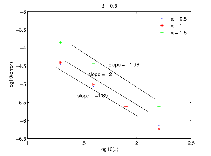
Replacing the RHS $-\mathbf{1}$ of the MET equation (2.8) by $\mathscr{L}(1+x^{2})_{+}$ given in (4.32) and (4.33), we have created a known solution $u(x)=(1-x^{2})_{+}$ . We compare the numerical solutions using our discretizations (3.30) and (3.31) (with the new RHS) against the analytical expression $u(x)=(1-x^{2})_{+}$ for different resolutions $J=20,40,80,160$ . Figure 2 shows that the numerical order of convergence based on the computed errors is close to two for all three values of $\alpha=0.5,1,1.5$ tested at the fixed point $x=-0.5$ . The convergence order is two, expected from the error analysis of our numerical method. In the verification, we have chosen $\beta=0.5,d=0,f\equiv 0,\varepsilon=1$ .

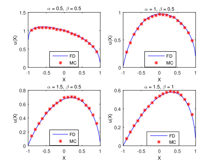
As a second verification, we compare our numerical solutions to the MET problem (2.8) and (2.9) with those obtained from solving the SDE (1.1) directly using Monte Carlo method. Both MET solutions are shown in Fig. 3 for $\beta=0.5$ or $1$ and $\alpha=0.5,1,1.5$ with $f\equiv 0,d=0$ and the domain $D=(-1,1)$ . To obtian the Monte Carlo solutions, we have taken $10,000$ sample paths and the time step size $\Delta t=0.001$ for each starting point $x$ within $D$ . The results in Fig. 3 show that the numerical solutions obtained from two different methods agree well. This numerical experiment demonstrates that our numerical method for computing the macroscopic quantities such as the MET is much more computational efficient than the Monte Carlo method, because our numerical error decreases quickly as the number of subintervals $J$ increases but the Monte Carlo solution converges slowly as the number of sample paths increases as expected. For comparing the computational costs of the two methods, we show the CPU time in Table 1 for the Monte Carlo method for the case we know the analytic solution for the MET: $\alpha=1.5,\beta=0,f\equiv 0,d=0,\epsilon=1$ . Table 1 shows that, in order to achieve the two-significant-digit accuracy in MET, one needs more than $8000$ sample paths and the CPU time for the Monte Carlo simulations is about $890$ seconds for one starting point $x=0$ while our method needs only $1.3$ seconds for $40$ starting positions and the error is less than $1.4\times 10^{-3}$ .

Table 1: The CPU times and the errors in the Monte Carlo simulation with

\alpha=1.5,\beta=0,f\equiv 0,d=0,\epsilon=1,x=0

sample paths	1000	2000	4000	8000
time(s)	95.9	163	320.6	891.8
Error( $10^{-2}$ )	4.12	1.64	1.03	0.81

To estimate the convergence orders for computing the MET, we take the numerical solution for the high resolution $J=1280$ as the ”true” solution. Figure 4 shows the errors of the solutions at $x=-0.5$ as $J$ increases from $10$ to $160$ by doubling, for different values of $\alpha=0.5,1,1.5$ , $\beta=0.5$ , $f\equiv 0$ , $d=0$ and $D=(-1,1)$ . According to the results, we find that our numerical method can only reach first-order accuracy and the numerical error for $\alpha=1.5$ is smaller than those in the cases of $\alpha=0.5,1$ . Unlike the previous solution $(1-x^{2})_{+}$ , the MET solution is known to have divergent derivatives at the boundary points. [8] Consequently, the error analysis in (3.28) does not apply as the derivatives of the solution are unbounded.

4.2 Mean exit time

For processes that are affected by asymmetric Lévy noise, little is known about the effects of the different factors in the Lévy noise on the MET. In this section, we examine the effects of the index of stability $\alpha$ , the skewness parameter $\beta$ , the size of the domain $(-b,b)$ , the drift $f$ , the intensity of Gaussian part $d$ and non-Gauassian part $\varepsilon$ of the noise. For odd drift functions $f(x)$ , as shown in Proposition 2.1, the solutions are symmetric when $\beta$ changes sign, i.e. $u_{-\beta}(-x)=u_{\beta}(x)$ . Thus, we will only present the results for $\beta\geq 0$ .

4.2.1 Effects of the skewness parameter $\beta$ and the index of stability $\alpha$

Figure 5 shows that the MET solutions for different values of $\beta=0,0.5,1$ for each of $\alpha=0.5,1$ and $1.5$ . In all cases shown, the domain is $D=(-1,1)$ and there is no drift $f\equiv 0$ and no Gaussian part $d=0$ . When $\beta=0$ , the MET $u$ is known, given by $\displaystyle{u(x)=\frac{\sqrt{\pi}}{2^{\alpha}\Gamma(1+\alpha/2)\Gamma((1+\alpha)/2)}(1-x^{2})^{\alpha/2}}$ , symmetric about $x=0$ just like the PDF $S_{\alpha}(1,0,0)$ displayed in Fig. 1. When $\beta\neq 0$ , the MET is not symmetric about $x=0$ even when the domain is symmetric. Furthermore, the larger $\beta$ is, the more asymmetric MET is. There are significant differences on the MET due to the effect of $\beta$ for different values of $\alpha$ . For $\alpha=0.5$ and $\beta=0.5$ or $1$ , we find that the METs $u(x)$ are discontinuous at the left boundary $x=-1$ , implying that the MET is nonzero once the starting point is insider the domain. The MET is smaller for larger value of $\beta$ if the starting point $x$ is positive, while the MET is much larger for bigger $\beta$ when the starting point is close to the left boundary. In contrast, the behavior changes for $\alpha=1$ or $1.5$ , as shown in Fig. 5(b) and (c): the MET is mostly smaller for larger value of $\beta$ for most of the starting points except when the starting point is close to the right boundary. These behaviors can be explained by examining the corresponding PDFs shown in Fig. 1. For example, the PDFs $S_{0.5}(1,\beta,0)$ in Fig. 1(a) show that it has almost zero probability moving to the left for $\beta=1$ , while the PDFs of $S_{1.5}(1,\beta,0)$ in Fig. 1(c) indicate that the stochastic process has larger probability moving to its immeadiate left when $\beta$ is larger.

To show the effect of index of stability $\alpha$ directly, Fig. 6 plots the METs for the fixed skew parameter $\beta=0.5$ but two different values of $\alpha=0.5$ and $1.5$ in one graph. For all starting point $x$ , the MET is smaller, skewed toward to the right and a continuous function of $x$ when $\alpha=1.5$ , while that of $\alpha=0.5$ is skewed toward the left and discontinuous at the left boundary. Compared with the PDFs of $S_{\alpha}(1,0.5,0)$ in Fig.1(b), the process for $\alpha=0.5$ has much smaller chance to move to the left, thus it takes longer time to exit the domain for the initial starting position in the left part of the domain.

4.2.2 Effect of domain size

Next, we increase the domain size to $D=(-4,4)$ and keep the other factors the same as in Fig. 5, i.e. $d=0,\varepsilon=1$ and $f\equiv 0$ for $\alpha=0.5,1,1.5$ . Comparing the results corresponding to the different domain sizes (the smaller size in Fig. 5 and the larger size in Fig. 7), we find that behaviors of the MET for different values of $\beta$ are similar for $\alpha=0.5$ and $\alpha=1.5$ . However, the profiles of the METs for $\alpha=1$ are dramatically different when the domain $D$ changes from $(-1,1)$ to $(-4,4)$ . For the larger domain, the process starting from the most of the left-half of the domain takes longer time to exit the domain when $\beta$ increases, while the opposite is true for the smaller domain. For the same value of $\beta$ , the shapes of the MET skewed toward the left for $D=(-4,4)$ instead of toward to the right for $D=(-1,1)$ .

4.2.3 Effect of noises

Now, let’s consider the effect of the intensities of the Gaussian noise, $d$ , and the non-Gaussian noise, $\varepsilon$ . Figure 8 shows the METs for different values of $d=0,0.1,1$ with the domain $D=(-1,1)$ , $\varepsilon=1,f\equiv 0$ and $\beta=0.5$ . The role of the Gaussian noises play on MET is obvious: when the noise is stronger, the MET is shorter for any $\alpha$ , similar to the results for the symmetric Lévy cases shown in [8]. If we add any amount of Gaussian noise (even for the low intensity $d=0.1$ ), the MET becomes continuous at the left end point when $\alpha=0.5$ . As the intensity of Gaussian increases, the MET is more symmetrical about the center of the domain $x=0$ .

Figure 9 shows the effect of the intensity of the non-Gaussian noise. From the METs for $\varepsilon=0.5,1$ with domain $D=(-1,1)$ , $\beta=0.5$ , $f\equiv 0$ and $\alpha=0.5$ and $\alpha=1.5$ , the MET gets smaller when $\varepsilon$ increases and the shape profile of the MET does not change much as we $\varepsilon$ changes.

4.2.4 Effect of drift term $f$

Last, we examine the effect of the O-U potential, i.e., having the drift term $f(x)=-x$ on the MET. Figure 10 shows the METs with the drift $f(x)=-x$ and without the drift $f\equiv 0$ for the case of pure non-Gaussian noise ( $d=0$ and $\varepsilon=1$ ). In the presence of the O-U potential, the MET increases as expected. For $\alpha=0.5$ , the MET $u(x)$ becomes discontinuous at both the boundary points of the domain, $x=1,-1$ when the O-U potential is added to the system. In contrast, the MET stays continuous for $\alpha=1.5$ when the drift term is present. Again, our numerical results demonstrate that the regularity of the solution appears to be dependent on whether $\alpha$ is greater than 1 or less than 1. It would be interesting research topic to investigate it theorectically.

4.3 Escape probability

First, we validate our equations (3.25) and (3.26) and the numerical implementation by comparing with analytical result for the special case of $f\equiv 0$ , $d=0$ , $\varepsilon=1$ and $\beta=0$ [8]

\displaystyle P_{E}(x)=\frac{(2b)^{1-\alpha}\Gamma(\alpha)}{[\Gamma(\frac{\alpha}{2})]^{2}}\int_{-b}^{x}(b^{2}-y^{2})^{\frac{\alpha}{2}-1}{\rm d}y.

(4.34)

Figure 11(a) and (b) show our numerical results match the analytical solution well for different domains, which verifies that our equations and the computer programs are correct.

Figure 11(c) and (d) tell us the effect of the skewness parameter $\beta$ on the escape probability of a process starting from the domain $D=(-1,1)$ , exiting the domain and landing first to the right $E=(1,\infty)$ . Here, we consider the pure jump Lévy process: $d=0,f\equiv 0$ and $\varepsilon=1$ . The results show that, when $\alpha=0.5$ , the escape probability is a sensitive function of $\beta$ and increases dramatically as $\beta$ changes from $-0.5$ to $0$ then to $0.5$ . In the contrast, when $\alpha=1.5$ , the process has less chance to escape the domain $D$ and first land in $E$ . The results are consistent with the plots of the probability density functions $S_{0.5}(1,\beta,0)$ and $S_{1.5}(1,\beta,0)$ shown in Fig. 1(a,c) and those of METs in Fig. 5. Here we note that, when $\alpha=0.5$ , the escape probability seems to be discontinuous at the left boundary point of the domain for $\beta=0.5$ and at the right boundary point for $\beta=-0.5$ . However, the probability is a continuous function of the initial position $x$ when $\alpha=1.5$ , agreeing with the results of MET presented earlier in the section.

Next, we consider the effect of the intensity of the Gaussian noise and the drift term on the escape probability in the case of asymmetric Lévy noise with $\beta=0.5$ . For $\alpha=0.5$ , Fig. 12(a) shows that, with any amount of the Gaussian noise, the escape probability becomes a smoother function eliminating any discontinuities at the boundary and it has larger effect for negative starting position $x$ than that for positive $x$ . The impact of the Gaussian noise is relatively small for $\alpha=1.5$ as shown in Fig. 12(b). Figure 13 shows that the difference in the drift term $f$ has a great influence on the escape probability. Recall that the drift term $f(x)=-x$ drives the process toward the globally stable point $x=0$ . Comparing with zero drift $f\equiv 0$ , we find that the probability with the drift term is smaller for the starting position $x>-0.3$ , while the escape probability with the drift is larger than that without the drift for the starting position $x<-0.5$ . Similar to the results of MET, the presence of the O-U potential $f(x)=-x$ causes that the escape probability be discontinuous at both end points of the domain.

5 Conclusions

For asymmetric Lévy motions, there are important applications in many fields, such as physics, mathematical finance and insurance risks. In addition, it attracts the attention of mathematicians because it is closely related to the nonlocal partial differential equations. In this work, an effective and convergent numerical algorithm has been developed for solving the mean first exit time and escape probability for one-dimensional stochastic systems with asymmetric Lévy motion. The convergence of the numerical method is verified numerically and the pointwise convergence order is closed to first-order. The numerical analysis predicts that the method is of second-order accuracy for smooth solutions. However, the numerical solutions have divergent derivatives or are discountinous at the boundary and therefore the convergence order suffers.

We also consider the influence of different parameters of the system on the mean exit time and the escape probability. For certain deterministic drift and symmetric domains, we find that the MET has a symmetry with respect to the skew parameter $\beta$ . Thus we focus on the case of $\beta>0$ and have seen that the profile of the MET becomes more asymmetric as $\beta$ is larger. From our numerical results, we find that, for $0<\alpha<1$ , the MET and the escape probability appear to be discontinous at the boundary of the domain but they are continuous for $\alpha>1$ . This interesting behavior of the solution worths further theoretical investigation.

6 Acknowledgements

The research is partially supported by the grants China Scholarship Council (X.W.), NSF-DMS #1620449 (J.D. and X.L.), and Simons Foundation #429343 (R.S.).

References

[1] D. Applebaum. Lévy Processes and Stochastic Calculus. Cambridge University Press, Cambridge, U.K., 2nd edition, 2009.
[2] J. Bertoin. On the first exit time of a completely asymmetric stable process from a finite interval. B. Lond. Math. Soc, 28(5):514–520, 1995.
[3] J. Bertoin. Exponential decay and ergodicity of completely asymmetric Lévy processes in a finite interval. Ann. Appl. Probab, 7(1):156–169, 1997.
[4] Z. Chen, R. Song, and X. Zhang. Stochastic flows for Lévy process with Hölder drifts. arXiv:1501.04758, 2015.
[5] Q. Du, M. Gunzburger, R. B. Lehoucq, and K. Zhou. Analysis and approximation of nonlocal diffusion problems with volume constraints. SIAM Review, 54(4):667–696, 2012.
[6] J. Duan. An Introduction to Stochastic Dynamics. Cambridge University Press, 2014.
[7] B. Dybiec, E. Gudowska-Nowak, and P. Hänggi. Lévy-Browmian motion on finite intervals: Mean first passage time analysis. Phys. Rev. E, 73:046104, 2006.
[8] T. Gao, J. Duan, X. Li, and R. Song. Mean exit time and escape probability for dynamical systems driven by Lévy noise. SIAM J. Sci. Comput., 36(3):A887–A906, 2014.
[9] M. Hao, J. Duan, R. Song, and W. Xu. Asymmetric non-Gaussian effects in a tumor growth model with immunization. Appl. Math. Model., 38:4428–4444, 2014.
[10] C. Hein, P. Imkeller, and I. Pavlyukevich. Limit theorems for p-variations of solutions of sdes driven by additive stable Lévy noise and model selection for paleo-climatic data. Interdiscip. Math. Sci., 8:137–150, 2009.
[11] Y. Huang and A. Oberman. Numerical methods for the fractional Laplacian: A finite difference-quadrature approach. SIAM J. Numer. Anal., 52(6):3056–3084, 2014.
[12] C. Kluppelberg. A continuous-time GARCH process driven by a Lévy process: stationarity and second-order behavior. J. Appl. Prob., 41(3):601–622, 2004.
[13] T. Koren, A. Chechkin, and J. Klafter. On the first passage time and leapover properties of Lévy mmotion. Physica A, 379:10–22, 2007.
[14] A. Lambert. Completely asymmetric Lévy processes confined in a finite interval. Ann. I. H. Poincare-Pr., 36(2):251 – 274, 2000.
[15] C. Li, F. Zeng, and F. Liu. Spectral approximations to the fractional integral and derivative. Fract. Calc. Appl. Anal., 15(3):383–406, 2012.
[16] X. Lü and W. Dai. Stochastic partial differential equations driven by fractional Lévy noises. arXiv:1410.09992v1, 2014.
[17] Y. S. Kim M. L. Bianchi, S. T. Rachev and F. J. Fabozzi. Tempered stable distributions and processes in finance: numerical analysis. Springer Milan, 2010.
[18] Z. Mao and J. Shen. Efficient spectral-Galerkin method for fractional partial differential equations with variable coefficients. J. Comput. Phys, 307, 2016.
[19] D. Middleton. Non-Gaussian noise models in signal processing for telecommunications: new methods an results for class A and class B noise models. IEEE T. Inform. Theory, 45(4):1129–1149, 1999.
[20] B. Podobnik, A. Valentincic, D. Horvatic, and H. Stabley. Asymmetric lévy flight in financial ratios. Proc. Natl. Acad. Sci. U.S.A., 108(11):17883¨C17888, 2011.
[21] J. Poirot and P. Tankov. Monte Carlo option pricing for tempered stable (CGMY) processes. Asia-Pac. Financ. Markets, 13:327–344, 2006.
[22] E. Priola. Pathwise uniqueness for singular SDEs driven by stable processes. Osaka J. Math., 49(2):421–447, 2012.
[23] H. Qiao and J. Duan. Asymptotic methods for stochastic dynamical systems with small non-Gasusian Lévy noise. Stoch. Dynam., 15, 2015.
[24] H. Qiao, X. Kan, and J. Duan. Escape probability for stochastic dynamical systems with jumps. In F. Viens, J. Feng, Y. Hu, and E. Nualart, editors, Malliavin Calculus and Stochastic Analysis, volume 34, pages 195–216, 2013.
[25] Y. Saad and M.H. Schultz. A generalized minimal residual algorithm for solving nonsymmetric linear systems. SIAM J. Sci. Stat. Comput., 7:856–869, 1986.
[26] G. Samorodnitsky and M. S. Taqqu. Stable Non-Gaussian Random Process. Chapman & Hall/CRC, 1994.
[27] K. I. Sato. Lévy Processes and Infinitely Divisible Distributions. Cambridge University Press, 1999.
[28] A. Sidi and M. Israeli. Quadrature methods for periodic singular and weakly singular fredholm integral equtaions. J. Sci. Comput., 3(2):201–231, 1998.
[29] X. Wang, J. Duan, X. Li, and Y. Luan. Numerical methods for the mean exit time and escape probability of two-dimensional stochastic dynamical systems with non-Gaussian noises. Appl. Math. Comput., 258(0):282 – 295, 2015.
[30] Y. Xu, J. Feng, J. Li, and H. Zhang. Lévy noise induced switch in the gene transcriptional regulatory system. Chaos, pages 1–11, 2013.
[31] Q. Yang, F. Liu, and I. Turner. Numerical methods for fractional partial differential equations with riesz space fractional derivatives. Appl. Math. Model., 34(1):200 – 218, 2010.

			$\displaystyle\int_{{\mathbb{R}}\setminus\{0\}}[u_{-\beta}(-x+y)-u_{-\beta}(-x)-I_{\{\|y\|<b\}}(y)\;yu_{-\beta}^{\prime}(-x)]\nu_{\alpha,-\beta}({\rm d}y)$
		$\displaystyle=$	$\displaystyle\int_{{\mathbb{R}}\setminus\{0\}}[\bar{u}(x-y)-\bar{u}(x)+I_{\{\|y\|<b\}}(y)\;y\bar{u}^{\prime}(x)]\left[\frac{C_{2}1_{\{0<y<\infty\}}+C_{1}1_{\{-\infty<y<0\}}}{\|y\|^{1+\alpha}}\right]\;{\rm d}y$
		$\displaystyle=$	$\displaystyle\int_{{\mathbb{R}}\setminus\{0\}}[\bar{u}(x+y^{\prime})-\bar{u}(x)-I_{\{\|y^{\prime}\|<b\}}(y^{\prime})\;y^{\prime}\bar{u}^{\prime}(x)]\left[\frac{C_{1}1_{\{0<y^{\prime}<\infty\}}+C_{2}1_{\{-\infty<y^{\prime}<0\}}}{\|y^{\prime}\|^{1+\alpha}}\right]\;{\rm d}y^{\prime}.$

Numerical algorithms for mean exit time and escape probability of stochastic systems with asymmetric Lévy motion

Abstract

1 Introduction

2 Concepts

2.1 Asymmetric Lévy motion

2.2 Mean exit time and escape probability

2.3 Symmetry and non-dimensionalization

Proposition 2.1 (Symmetry of Solutions).

Proof.

3 Numerical methods

3.1 Reformulation

3.2 Discretization

4 Numerical results

4.1 Validation

4.2 Mean exit time

4.2.1 Effects of the skewness parameter β\beta and the index of stability α\alpha

4.2.2 Effect of domain size

4.2.3 Effect of noises

4.2.4 Effect of drift term ff

4.3 Escape probability

5 Conclusions

6 Acknowledgements

References

4.2.1 Effects of the skewness parameter $\beta$ and the index of stability $\alpha$

4.2.4 Effect of drift term $f$