Dominance Move: A Measure of Comparing Solution Sets in Multiobjective Optimization
Abstract: One of the most common approaches for multiobjective optimization is to generate a solution set that well approximates the whole Pareto-optimal frontier to facilitate the later decision-making process. However, how to evaluate and compare the quality of different solution sets remains challenging. Existing measures typically require additional problem knowledge and information, such as a reference point or a substituted set of the Pareto-optimal frontier. In this paper, we propose a quality measure, called dominance move (DoM), to compare solution sets generated by multiobjective optimizers. Given two solution sets, DoM measures the minimum sum of move distances for one set to weakly Pareto dominate the other set. DoM can be seen as a natural reflection of the difference between two solutions, capturing all aspects of solution sets’ quality, being compliant with Pareto dominance, and does not need any additional problem knowledge and parameters. We present an exact method to calculate the DoM in the biobjective case. We show the necessary condition of constructing the optimal partition for a solution set’s minimum move, and accordingly propose an efficient algorithm to recursively calculate the DoM. Finally, DoM is evaluated on several groups of artificial and real test cases as well as by a comparison with two well-established quality measures.
Keywords: multiple criteria, quality measure, metaheuristics
1 Introduction
In multiobjective optimization, it is often desirable for search algorithms to provide the decision maker (DM) with a representative subset of the whole Pareto-optimal (efficient) frontier. This largely avoids overload from both the computational and decision-making perspectives [1, 2, 3, 4]. Over the past several decades, a variety of search techniques (called multiobjective optimizers here) have emerged ranging from exact methods to heuristics or metaheuristics [5, 6, 7, 8], aiming at finding a “good” representation of the Pareto-optimal frontier. However, the meaning of “good” is ambiguous [9]. There is no clear definition in the operations research and optimization community of what a good representation of the Pareto-optimal frontier should be. This naturally leads to a question — how to evaluate and compare the quality of solution sets obtained by different multiobjective optimizers.
Quality evaluation of solution sets in the context of multiobjective optimization has gained wide attention in both the operations research and computational intelligence areas [10, 11, 12, 13, 9]. [10] considered the analytical evaluation of the solution quality of multiobjective heuristics, and defined approximation errors as the value penalty incurred by approximating a Pareto-optimal solution with its heuristic alternative. [14] proposed three metrics, coverage error, uniformity level and cardinality, to evaluate the coverage of a solution set to the Pareto-optimal frontier, the uniformity among solutions in the set and the number of solutions in the set, respectively. To evaluate a solution set’ quality in terms of both convergence and diversity, [15] measured the volume of the objective space enclosed by the set and a reference point. This is the well-known hypervolume metric. [16] considered the convergence of a solution set to the Pareto-optimal frontier and defined generational distance (GD) by calculating the average distance from all solutions in the set to the optimal frontier. Later, GD was modified in reverse by considering the distance from the optimal frontier (represented by a reference set) to the solution set, called inverted generational distance (IGD) [17]. This measure can reflect both convergence and diversity of a solution set. [18] introduced the integrated preference functional (IPF) to measure the quality of a solution set for biobjective optimization problems. In their work, the form of the decision maker’s value function was represented as a convex combination of objectives, and thus only supported points contribute to the IPF result. Later, [19] presented an extension of the IPF for general -objective optimization problems. Recently, [20] considered the weighted Tchebycheff function for the calculation of the IPF measure, thus counting all nondominated points (both supported and unsupported) of a solution set. On the other hand, [12] carried out theoretical study of quality measures. They analysed theoretical limitations of unary quality measures (i.e., the measure that assigns one solution set a numerical value that reflects a certain quality aspect), and stated the strengths of binary quality measures (i.e., the measure that directly uses a numerical value to describe how much better one solution set is than another).
Despite the activity of the design and analysis of quality evaluation techniques, evaluating solution sets encounter various difficulties in practical applications [21, 22, 20]. Some measures evaluate only one aspect of a solution set’s quality, such as GD. Many measures do not comply with the Pareto dominance relation of two solution sets [23]. This happens a lot in those measures which solely evaluate the diversity of a solution set [24]. In addition, the Pareto-optimal frontier (or its substituted set) of a given problem is often required to compare solution sets, such as in the coverage error, GD, IGD, and Daniels’ approximation errors measure. This, however, is commonly unavailable in practice. Moreover, some quality measures require additional problem knowledge in the evaluation of solution sets, for example, the reference point in the hypervolume metric and the ideal point in the Tchebycheff-based IPF. This may affect the evaluation results, especially when comparing several solution sets with different spatial locations [25]. Finally, parameter setting is an important issue in those parameter-dependent quality measures. In such measures, the accuracy of evaluation results depends largely on a proper choice of the parameter(s); also, the sensitiveness is often affected by the cardinality of a solution set and the dimension of its solution vectors.
In this paper, we propose a new quality measure, called dominance move (DoM), to compare solution sets obtained by multiobjective optimizers. DoM measures the minimum sum of move distances needed to make a set (weakly) Pareto dominate another set. It is able to capture all aspects of solution sets’ quality, i.e., the closeness to the Pareto-optimal frontier, the extensity of the solution set covering, the uniformity among solutions in the set, and the number of nondominated solutions in the set. Moreover, DoM is Pareto compliant and does not need any additional problem knowledge and parameters. Most importantly, the proposed measure is of highly intuitive — it can be seen as a natural reflection of the differences between solution sets.
We present an exact calculation method for the DoM measure in the biobjective case. We show the necessary condition of constructing the optimal partition for a solution set’s minimum move, and accordingly propose an efficient algorithm (with the computational complexity where is the cardinality of the set) to calculate the DoM result.
The rest of this paper is structured as follows. In §2, we give the main notations and terminology used and introduce some related work. Section 3 is devoted to the description of the proposed DoM. We present an exact method to calculate the DoM measure in §4. Section 5 evaluates DoM, including several artificial examples to develop the reader’s intuition, a comparison study with popular quality measures, and two practical examples on combinatorial and continuous optimization problems. Finally, concluding remarks are provided in §6.
2 Preliminaries and Related Work
In this section, first we briefly introduce several definitions that are used in the comparison between solutions and accordingly between solution sets. We then review some quality measures in the literature.
2.1 Terminology
Without lost of generality, we consider a minimization problem with objective functions , . The objective functions map a point in the decision space to an objective vector in the objective space . In view of that in most case only objective vectors are considered in quality evaluation, we only define the comparison relation based on objective vectors. In addition, for reasons of simplicity we refer to an objective vector also as a solution (despite it being originally called in ) and the outcome of a multiobjective optimizer as a solution set.
Let two solutions . Solution is said to weakly dominate (denoted as ) if and only if for . If there exists at least one objective on which , we say that dominates (denoted as ). A solution is called Pareto optimal (efficient) if there is no other that dominates . The set of all Pareto optimal solutions of a multiobjective optimization problem is called its Pareto-optimal frontier.
The relation between solutions can be naturally extended to solution sets [12]. Let two solution sets . Solution set is said to weakly dominate (denoted as ) if every solution is weakly dominated by at least one solution . If for every solution there exists at least one solution that dominates , we say that dominates (denoted as ). We can see that the weak dominance relation between two sets does not rule out their equality, while the dominance relation does completely. There thus exists another situation that weakly dominates but does not equal . That is, every solution in is weakly dominated by one solution in but there is at least one solution in that is not weakly dominated by any solution in (i.e., ). This relation represents the most general and weakest form of superiority between two solution sets and was defined as being better (denoted as ) in [12]. Put it simply, means that is at least as good as , while is not as good as .
2.2 Related Work
With the development of effective search techniques in multiobjective optimization, the issue of quality evaluation has become increasingly important. Over the past several decades, a large number of quality measures have been emerging not only in the operations research [26, 27] and evolutionary computation fields [28, 29, 21], but also in other fields such as mechanical design [30, 31] and software engineering [32].
As the most general form of preference between solution sets in multiobjective optimization, the Pareto dominance relation has naturally been considered in solution sets’ quality comparison. However, in most cases this comparison is not feasible in practice. On the one hand, solution sets obtained by multiobjective optimizers are typically non-dominated to each other. On the other hand, people may be interested in more precise statements that quantify the difference between solution sets.
An alternative is to consider the dominance relation between solutions from different sets (rather than between sets). For example, [33] compared two solution sets by the number of solutions in one set that are not dominated by any solution in the other set. [14] counted the number of nondominated solutions in the obtained set. However, this comparison cannot provide any information of solution sets’ distribution (e.g., the coverage of solution sets over the Pareto-optimal frontier). In addition, solutions between the sets become increasingly incomparable as the number of objectives in optimization problems grows.
[14] also considered the distribution of a subset of the Pareto-optimal solutions, introducing two quality measures, coverage error and uniformity level. The former measures the coverage of the set to the optimal frontier, and the latter quantifies the distance between neighboring points in the set. These measures, however, only work on the Pareto-optimal solutions and thus are infeasible for solution sets obtained by heuristics. Similarly, some popular quality measures in evolutionary multiobjective optimization, such as GD [16], IGD [17] and their variants [34, 35, 36], require a reference set that well represents the Pareto-optimal frontier of the problem in their evaluation process. However, it is difficult to specify such a reference set without the knowledge of the Pareto optimal frontier. Different reference sets can easily lead to inconsistent evaluation results between the solution sets [37].
[18] introduced a quality measure based on the integrated preference functional (IPF), without the requirement of the knowledge of the Pareto-optimal frontier. This measure used partial information on the decision maker’s value function and was designed for biobjective optimization problems. Later, [19] extended this IPF measure, enabling it feasible for general -objective optimization problems. However, since the the form of the decision maker’s value function was represented as a convex combination of objectives, only supported points in a solution set contribute to the IPF result. To address this issue, [20] considered the weighted Tchebycheff function as the value function in IPF, which makes the evaluation result include the information of unsupported points. This modification introduces an additional parameter, the ideal point (for the calculation of the Tchebycheff function), which may affect the evaluation result to some extent.
As a well-known measure for approximation algorithms in operations research and theory [38, 39, 40, 41] as well as evolutionary multiobjective optimization [42, 43], the -approximation can naturally be used to quantitatively compare solution sets. [12] presented an -approximation based measure (called indicator) with two versions, additive indicator and multiplicative indicator. Here, we consider the additive indicator and similar results can be found in the multiplicative version. For two solution sets and , the additive indicator is the minimum value that can be added to each solution in such that they become weakly dominated by at least one solution in . Formally, the additive indicator is calculated as
| (1) |
where denotes the objective value of solution in the th objective and is the number of objectives.
 |
 |
| (a) Solution set | (b) Solution set |
As pointed out by [12], the indicator has some desirable features, such as no need of a reference set, complying with the Pareto dominance relation, and representing natural extension to the evaluation of approximation schemes in operations research and theory. However, one weakness of the indicator is that its evaluation result is only related to one particular solution in either solution set. This could lead to an inaccurate evaluation of quality comparison between solution sets. Figure 1 gives an example that the indicator fails to distinguish between solution sets ( and ). As can be seen from the figure, has more solutions and a better coverage over the Pareto-optimal frontier than , but the two sets have the same comparison result ().
In addition, the indicator only considers one particular objective in comparing the difference between two solutions (i.e., the objective on which one solution performs worst relative to another solution). This ignores the difference on other objectives and naturally leads to an information loss. This information loss becomes more severe as the number of optimization problems’ objective increases. Consider two 10-objective solutions, and . Solution performs better on nine objectives and solution better only on the last objective, but they have same comparison result ().
 |
 |
| (a) With reference point | (b) With reference point |
The hypervolume (HV) metric [15] is one of the most popular quality measures in multiobjective optimization. It calculates the volume of the space enclosed by a solution set and a reference point, and a large value is preferable. The HV of a solution set can be described as the Lebesgue measure of the union hypercubes defined by and the reference point :
| (2) |
where ( for all ).
The HV indicator has good theoretical properties [12] and can give a comprehensive evaluation of a solution set in terms of both convergence and diversity. While the computational complexity of calculating HV increases exponentially with the number of objectives, the Monte Carlo sampling method can provide a good balance between accuracy and running time [44, 45]. However, the HV indicator is sensitive to the choice of the reference point. How to choose a proper reference point is not trivial and different reference points can lead to inconsistent evaluation results [23]. Take two solution sets ( and ) in Figure 2 as an example. When the reference point is set to (Figure 2(a)), . When the reference point is (Figure 2(b)), .
3 The Proposed Measure
Dominance move (DoM) is a measure of comparing two sets of multi-dimensional points (i.e., vectors). It considers the move of points in one set to make this set weakly dominate the other set. DoM can be defined as follows.
Definition 1.
Let be a set of points and be a set of points . The dominance move of to (denoted as ) is the minimum total distance of moving points of such that any point in is weakly dominated by at least one point in . That is, we move to positions 11 1 If keeps still, we can regard it as . (thus constituting ) such that 1) weakly dominates and 2) the total of the move from to is minimum.
Mathematically, DoM can be expressed as
| (3) |
| (4) |
where , , denotes the value of solution in the th objective, and is the number of objectives.
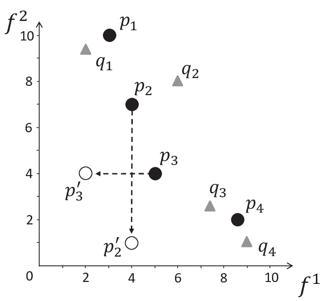
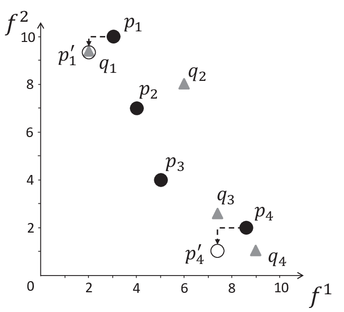
Apparently, to make , any point either stays still or moves to a “better” position (i.e., ). There are numerous ways to make this move. For example, we could move only one point of to make it cover (weakly dominate) all points in ; we could also move some points of to make them together cover all points in ; or we could directly consider the minimum move of ’s points to each point of . Figure 3 gives three examples of this move. In Figure 3(a), moves to the position to cover all four points of . In Figure 3(b), and move to and to cover and , respectively. In Figure 3(c), and move to and to cover and , respectively, in view of that is already covered by one point of .
 |
 |
 |
| (a) Total move of is | (b) Total move of is | (c) Total move of is |
Out of numerous possibilities of the above move, the dominance move corresponds to the one that has the minimum distance. This minimum distance reflects how far one solution set () needs to move to cover another solution set (). In other words, it indicates performance inferiority of to (i.e., the advantage of over ). It is clear that is always larger than or equal to . A small value indicates that performs well relative to . This implies the quality in both convergence and diversity. A small means that for each point of (whatever its location), there exists at least one point of that only needs a little move at most to cover it. Take Figure 3 as an example, where the dominance move corresponds to the case of Figure 3(c). As can be seen, has a good coverage over since only a little move of its points is needed to (weakly) dominate any point of . In addition, if then .
It is worth noting that the well-known indicator also measures the minimum value added to one solution set to make it be weakly dominated by another set. However, it only considers one particular solution in either solution set. This inevitably leads to information loss of the comparison between the two sets. For the example in Figure 3, the indicator () would only measure the advantage of over , regardless of the difference between the remaining solutions of the two sets. A comparative test will be carried out later (Section 5.2) to demonstrate the difference between the proposed DoM and the indicator (as well as other quality measures). In the following, we present several properties of DoM which can help further understand its behavior.
Proposition 1.
Let solution sets and points . Then the following facts are true:
(a) .
(b) (i.e., , see Section 2.1) .
(c) and .
(d) Let and . If , then . Also, if or , then .
(e) If , then and .
(f) and .
Proof.
Proof. Facts (a)–(d) follow directly from the definition of the dominance move.
(e) By the definition of , for any point , there exists one point moving to to weakly dominate in . Since , for point there exists one point which weakly dominates . This means that the value of any objective of point is either equal to or smaller than that of point . Therefore, the move distance from to is equal to or smaller than that from to . Given this and , we can construct a move for to weakly dominate whose total distance is equal to or smaller than . In addition, by the definition of the dominance move, this distance is greater than or equal to . Thus .
The second inequality is proven analogously.
(f) Let be the new position to which moves in . Then . By Fact (e) above, follows. Let be the position to which moves in . Now, we can obtain a path from to and then from to (for to weakly dominate ), whose move distance is equal to or smaller than . Likewise, by the dominance move definition, this distance is greater than or equal to . Thus .
The second inequality is proven analogously. ∎
Fact (b) implies a desirable property of the proposed measure in comparing two solution sets: whenever one solution set is better than another set , then . Fact (e) implies the relation of two solution sets when they are individually compared with a third set. That is, if , then will not be (weakly) dominated by ; if , then will not be (weakly) dominated by .
When considering the move of to cover , any will be associated with a point (i.e., moving to somewhere to weakly dominate it). This is like a partition in the sense that the set is partitioned by points of into some groups22 2 In principle, one point of could be put into more than one group. However, this will naturally lead to a longer distance for to move. So here for brevity we only consider one point of being in one group. (subsets) such that the union of these groups is and each group corresponds to only one point of . For example, in Figure 3(a), all points of are put into one group corresponding to . In Figure 3(b), () and () can be seen to be put into two groups corresponding to and , respectively. In Figure 3(c), (), () and () can be seen into three groups corresponding to , and , respectively.
After a partition is created, for one group (denoted as ), its corresponding point needs to move to somewhere to weakly dominate all points in . The minimum distance of this move is equal to the distance from to the ideal point33 3 The ideal point of a set of points is constructed by the best value of each objective for all points in the set. of and (denoted as ). Formally, it can be expressed as
| (5) |
where , denotes the objective value of point in the th objective, and is the number of objectives.
In fact, can also be seen as the dominance move distance of one point () to a set (); i.e., when , . Additionally, when (i.e., ), means the dominance move of point to point , namely, . Note that in the calculation of the dominance distance (Equations (4) and (5)), the move of the points is based on the Manhattan distance ( norm). In principle, other distance metrics, such as Euclidean distance, could also be used. We here consider the Manhattan distance in views of its desirable properties. On the basis of the measure of the Manhattan distance, when adding one point to an existing group associated with , the additional move can be calculated by a direct comparison between and . This indicates that we do not need to consider the order of points of entering a group. In other words, for a group , a point can successively “access” (i.e., move to somewhere to cover) the points of in any order, and the total move distance is always the same (namely, the distance of the move from to directly).
The following proposition gives the connection with respect to the dominance move when adding a set of points into an existing group .
Proposition 2.
Let and be two solution sets, and . Then the following equality holds for any point :
| (6) |
where denotes the ideal point of set .
Proof.
Proof. By Equation (5), we have
where denotes the objective value of point in the th objective, and is the number of objectives. ∎
Corollary 1.
The above results have presented properties of the dominance move of one point of to the groups which is partitioned into. Next, we redefine the dominance move of to from the perspective of the partitioning.
Definition 2.
Let solution sets . We call to be a partition of to if , where and . Then the dominance move of to corresponds to the partition satisfying that is minimum. We call this partition an optimal partition of to .
Note that there can be more than one partition satisfying that is minimum. So, we may have several optimal partitions of to . From the above definition, the proposed measure is transformed into a problem of finding an optimal partition of to . This partitioning problem has an important property below.
Theorem 1.
Let be a partition of one set to another set . Let be the set of ’s points of one or several groups in . Now if we can find a partition of to with a smaller dominance move than the original group(s) in , then we can construct a smaller partition of to than .
Proof.
Proof. Let the original partition of to in be , and the new smaller partition of to be . Then and . Let be the original groups associated with in . Now we have that
where the last inequality is obtained by Corollary 1. This means that the points of the groups in can be repartitioned by with a smaller dominance move (since ). This will lead to a new partition of to with a smaller dominance move as long as we keep the other groups in the original unchanged. ∎
This theorem indicates that if merging or splitting some groups can lead to a smaller partition of them, then these groups do not exist in any optimal partition. This further results in several properties of the optimal partitioning.
Corollary 2.
Let be an optimal partition of a solution set to another set , and ( associated with ) be one of the groups obtained by this partition. Then the following facts are true:
(a) If (i.e., ), then .
(b) Considering the optimal partitioning of to , keeping with corresponds to an optimal partition of them.
(c) When , let be two points in . In there may exist some points “between” and (i.e., being weakly dominated by ). Then categorizing such points into corresponds to an optimal partition of to .
Proof.
Proof. Facts (a) and (b) follow directly from Theorem 1 (by contradiction).
(c) Let a point between and be in another group (associated with ) of . By Proposition 1(c), . Since is weakly dominated by , ( being the position for to move to cover ). It follows that . Therefore, . Since is already an optimal partition, by Theorem 1, and transferring from to is also an optimal partition of to . ∎
Fact (a) presents the determinacy of the groups’ associated point in an optimal partition when their cardinality is one. Fact (b) shows that the optimal substructure holds in this optimal partitioning, and Fact (c) provides a sufficient condition for points to enter a group after given two points belonging to this group in an optimal partition.
4 Calculating DoM in the Biobjective Case
In this section, we present a method to calculate the DoM measure in the biobjective case. Before introducing the calculation procedure, for convenience we define a term with respect to points’ relationship in a set based on the dominance move.
Definition 3.
Let be a set of points, and . We call a point () the inward neighbor of in (denoted as ) if has the smallest dominance move distance to ; that is, .
Consider two sets of two-dimensional points, and . The dominance move of to can be calculated by four steps below. Step 1 removes the points that do not affect . Step 2 is the first attempt of constructing an optimal partition of to . Step 3 tests whether it is an optimal partition or not. If not, Step 4 recursively merges points of to make all points of eventually associated with one point in .
Step 1. Remove the dominated points in both and , respectively, and remove the points of that are dominated by at least one point in .
It is clear that these points have no effect on the result of (Fact (d) of Proposition 1). So now in the union set of and , there is only one possibility of two points subject to the dominance relation: a point from being dominated by a point from .
Step 2. Denote . First we regard each point of in as a group. Then for each point of , find its inward neighbor in ; that is, , find a point such that . If the point , then merge into the group of . For the case that the point , if and are already in one group, do nothing; else merge the two groups of and into one group.
Now we can see that each point of and its inward neighbor belong to one group.
Step 3. If there exists no point such that (i.e., two points are the inward neighbor of each other) in any group, then the procedure ends; these groups construct an optimal partition of to (which will be presented in Theorem 2 below). Otherwise, the procedure continues.
Now, we show that Step 2 constructs an optimal partition of to provided that satisfying that in any group. To prove this, we first present that it is a partition of to (i.e., in each group there is one and only one point belonging to ).
Lemma 1.
Let and be two sets of nondominated points in the biobjective case. Place each point of and its inward neighbor in into the same group by Step 2. The resulting groups construct a partition of to provided that in any group.
Proof.
Proof. First, we can see from Step 2 that in any group there is no more than one point of . Now we only need to present that there is at least one point of in each group. Apparently, if there is no point of in one group, some points in this group will form a directed circle whose edges are the dominance move of their inward neighbor to themselves (since the number of the points is equivalent to that of the edges). The case that can be seen as the circle having only two vertexes. Next, we prove (by contradiction) that in any group there exists no such a circle having more than two vertexes.
Assume that there exists one group, in which some points form a directed circle. Let these points be (where ), and also suppose that they are sorted with their first objective, i.e., . Since they are nondominated to each other, we have that for the second objective. It follows that the inward neighbor of is . This implies that is the inward neighbor of since these points form a directed circle. However, by , we have that . Hence, is not the inward neighbor of , a contradiction. ∎
Now we present that this partition is an optimal partition.
Theorem 2.
The partition of to formed by grouping each point of and its inward neighbor in is an optimal partition of to .
Proof.
Proof. (By contradiction) Assume that the partition formed by grouping each point of and its inward neighbor is not an optimal partition. Then we can find an optimal partition in which there exists at least one point and its inward neighbor not being in the same group. Let in belong to the group (associated with ) and its inward neighbor ( or ) belong to the group (associated with ). Next, according to the relation of points and (whether weakly dominates or not), we consider two situations separately.
For the first situation that , by Proposition 6 and (the definition of the inward neighbor), we have
Since , it follows that . By this and Fact (f) of Proposition 1, the above inequality can be expressed as
If , then (Lemma 1). We thus have that , a contradiction with being an optimal partition (Theorem 1). If , add into both sides of the above inequality. By Proposition 6 and Fact (f) of Proposition 1, we have
A contradiction follows immediately from Theorem 1, thus completing the proof for the situation that .
Now let us consider the second situation that . Obviously, (otherwise is the inner neighbor of ). Without loss of generality, let be below (i.e., be smaller than on the second objective). Since is the inner neighbor of , the advantage of over on the first objective will be greater than . On the other hand, according to the position of the points of relative to , we divide them into three subsets , , and (), where consists of the points above and below . By Proposition 6, we have
Since both and are below and is the inner neighbor of , the advantage of over the ideal point of and on the first objective is still greater than , namely . Considering , since is above , and is above and nondominated with and , it follows that . Substituting these in the above equality, we have
If , then and a contradiction directly follows from . If , add into both sides of the inequality. By Proposition 6 and Fact (f) of Proposition 1, we have
A contradiction (by Theorem 1). This completes the proof of the second situation. ∎
From the proof of the above claim, we further have
Corollary 3.
In all possible optimal partitions of to in the biobjective case, any point of and its inward neighbor in are in the same group.
Step 4. For any group that has a circle (i.e., two points being the inward neighbor of each other), replace these two points by their ideal point. This leads to a new (denoted as ). Then find the inward neighbor of such an ideal point in and group them. Go to Step 3.
This step updates the groups which have no point belonging to . This update will not affect the inner neighbor of the points of .
Proposition 3.
Let and be two sets of nondominated points in the biobjective case, and a pair of points be the inward neighbor of each other in . Let be the ideal point of , and . Then, replacing with will keep the inner neighbor of any other points of unchanged. That is, for (), if or , then ; if (), then .
Proof.
Proof. To prove this, we only need to present that for any point (), . This implies that if the inner neighbor of is neither nor , replacing and with will not change its inner neighbor; if the inner neighbor of is or , will be its inner neighbor. Since and are nondominated in the two-dimensional space and they are the inner neighbor of each other, there is no point between them. That is, some points of are above them and the others below them. Without loss of generality, let be above . Thus for any point above , we have that . Likewise, for any point below , . Hence, for any point , . This completes the proof of the claim. ∎
The above claim indicates that directly grouping and its inner neighbor will form a set of groups satisfying that any point of and its inner neighbor in being in the same group. Next, we give the connection of the optimal partitioning of to and the optimal partitioning of to .
Theorem 3.
If is an optimal partition of to , then will be an optimal partition of to , and also .
Proof.
Proof. We denote as the sum of the dominance move distances of the partition . Since is an optimal partition of to , . Denote in as the ideal point of and in . Apparently, splitting into and in leads to a partition of to . Now we present is an optimal partition of to .
Assume that is an optimal partition of to , namely . By Corollary 3, and are in one group, denoted as (associated with ), in . Replacing and with their ideal point leads to a partition of to (). Since is an optimal partition of to , . On the other hand, since is the ideal point of and , by Equation (5), we have that . It follows that . Likewise, . Therefore,
This means that is an optimal partition of to , and also . ∎
This theorem, coupled with Theorem 2, ensures that by recursively removing the circle in newly-generated groups (in order to make them associated with one point of ), the final formed partition corresponds to an optimal partition of to .
Next, we consider the computational complexity of the procedure. For simplicity, let both and have the same cardinality (i.e., ). According to [46], removing the dominated points for the biobjective case (Step 1) requires comparisons. In the biobjective case, the inner neighbor of the points of should be in the range determined by their left and right neighbors in . Therefore, it only needs to check a constant number of points (three on average) to find the inner neighbor of one point of . So the operations of Step 2 require comparisons. Since at most () circles are generated, the recursion of Steps 3 and 4 happens at most () times. Likewise, finding the inner neighbor of a newly-generated ideal point requires a constant number of comparisons (also no need to update the inner neighbor of other points of according to Proposition 3). Thus, the operations in Steps 3 and 4 require comparisons. To summarize, the overall computational complexity of the procedure is .
To illustrate the proposed method, Figure 4 gives an example of calculating the DoM measure stepwise. The considered sets and respectively have five points, shown in Figure 4(a). By Step 1, has been removed (Figure 4(b)) since it is dominated by one point of . Then, Step 2 finds the inner neighbor of the points to (which is and , respectively) and groups them together. This is shown in Figure 4(c). Since and form a directed circle, replace them by their ideal point (Figure 4(d)). And then find the inner neighbor of : . This however leads to another circle of and . Remove this circle by replacing and by their ideal point (Figure 4(e)). And find the inner neighbor of : . Now the three points are in one group. This results in a partition of to that the points are associated with . Therefore, the dominance move is the distance from to ( moving to to dominate ), which is shown in Figure 4(f).
 |
 |
 |
| (a) | (b) | (c) |
 |
 |
 |
| (d) | (e) | (f) |
Finally, it is necessary to note that calculating the DoM measure for more than two objectives may become an intractable task. The method proposed here cannot apply to such cases directly. The property that points and their inner neighbor are always in the same group in an optimal partition (Theorem 2 and Corollary 3) does not hold in general. For example, let and be two sets of tri-dimensional points: and . The inner neighbor of points , and is , and , respectively. This forms a partition of to with the dominance move distance being . However, if we directly move to the position to dominate all the three points of , we can obtain a smaller move distance (), which is in fact an optimal partition of to .
5 Experimental Studies
In this section, we evaluate the proposed DoM measure. First, several groups of artificial test cases are introduced to test the effectiveness of DoM in reflecting a variety of quality aspects. Then, a comparison of DoM with two well-established quality measures, HV and the indicator, is made. Finally, DoM is examined further on two realistic problem instances, one combinatorial and the other continuous.
5.1 Artificial Examples
In general, the quality of solution sets in multiobjective optimization includes three aspects: convergence, diversity, and cardinality. Convergence measures the closeness of a solution set to the Pareto-optimal frontier, diversity quantifies the distribution of a solution set over the optimal frontier, and cardinality counts the number of (non-dominated) points in a solution set. Diversity can be further divided into two sub-aspects [14]: uniformity and extensity. The former considers the distance between points in a solution set and the latter measures the range of a solution set covering. A comprehensive quality measure is expected to be capable of capturing all these aspects.
In this section, we consider four groups of test cases to evaluate DoM in convergence, uniformity, coverage and cardinality, respectively. We construct these test cases in such a way that it is evident which solution set is better than the other in one specific aspect of solution quality. That is, in each test case the difference of the two sets lies in only one aspect; in the other three aspects they perform equally.
 |
 |
| (a) | (b) |
Consider convergence first. Pareto dominance is a central criterion in reflecting the convergence of solution sets. As we know, DoM complies with the Pareto dominance criterion. For two solution sets and , if (weakly) dominates , (Fact (b) of Proposition 1). If dominates some points of and does not dominate any point of , the DoM measure is likely to prefer to (i.e., ). Figure 5(a) is such an example, where some points of are dominated by points in and the two sets have same quality in the uniformity, extensity and cardinality aspects. As seen, the dominance move of to is less than that of to (0.50 vs 0.68).
Now one may ask what if two solution sets are nondominated completely to each other. Figure 5(b) is an example to illustrate this situation. In this example, we first generate a well-distributed set , and then generate through moving to the upper left a little. Specifically, for a point , the corresponding point is generated by and , where denotes the objective value of point in the th objective. By this, any point in the two sets is nondominated, but may be seen to have a better convergence than (in view of the way generating ), which is consistent with the DoM result (). This indicates that the DoM measure prefers the set with better convergence, even when the two sets are incomparable in terms of the dominance relation of their points.
 |
 |
| (a) | (b) |
The solution sets in Figure 6 are used to test DoM in terms of distribution uniformity. Each pair of sets have the same convergence (set being shifted by 0.2 on both objectives in the figure for a better observation), extensity, and cardinality. Set in each pair is distributed uniformly. Set in Figure 6(a) is distributed randomly in the range of set , and in Figure 6(b) the distance between neighboring points in set increases gradually from bottom to top. As can be seen in the figure, the evaluation results of DoM indicate its preference for a set of uniformly-distributed points.
 |
 |
| (a) | (b) |
The two examples in Figure 7 test DoM in evaluating the distribution extensity of solution sets. In both examples, set is a well-distributed set, with the range of on both and objectives. In Figure 7(a), set is generated by shrinking a little, resulting in its range being on both objectives. In Figure 7(b), set is distributed uniformly in the range of the five bottom right points of , and thus its range is . As shown, DoM is able to accurately reflect the extensity of solution sets — a set with better extensity has a smaller dominance move to its competitor.
 |
 |
| (a) | (b) |
Figure 8 verifies the DoM measure in evaluating the cardinality of solution sets. In Figure 8(a), the two sets perform equally in terms of convergence, uniformity and extensity, but set has one more point than , thus being preferred by DoM (). Figure 8(b) is an interesting case, where set is generated by adding two new points to which is a set of uniformly-distributed points. This causes that has a worse uniformity than . However, provides more information to the decision maker than , and should be considered better. In fact, weakly dominates but does not. The DoM result can reflect this information: .
5.2 Comparison with Other Quality Measures
In this section, we compare DoM with two popular quality measures in multiobjective optimization, the indicator and HV. As described in Section 2.2, these two measures have some desirable features and both aim to provide a comprehensive evaluation of solution sets’ quality.
In this comparison, we consider the solution set examples from Figures 1 and 2 in Section 2.2, where the indicator and HV fail to accurately compare the sets, respectively. This allows us to see if the proposed measure is able to provide a reliable result on the examples where its peers struggle.
Table 1 shows evaluation results of the three measures. For the example in Figure 1, set has a better distribution and more points than set , but the indicator cannot distinguish between them (). In contrast, the HV and DoM measures can accurately reflect the difference of the two sets, with having a better evaluation result always.
| Two sets | Hypervolume | indicator | DoM |
|---|---|---|---|
| vs in Figure 1 | 52 vs 47 | 1.0 vs 1.0 | 1.0 vs 4.0 |
| vs in Figure 2 | 48 vs 49 | 2.0 vs 2.0 | 2.0 vs 4.0 |
For the example in Figure 2, two points in set are dominated by set . Clearly, provides more information than and is likely to be preferred by the decision maker. However, the HV evaluation result on these two sets depends on the choice of the reference point. If the reference point is set to , set will be preferred by HV to . When the two sets are compared using the indicator, the evaluation results are identical (). This is because the indicator only considers the difference on one particular objective of one particular point of either solution set. In contrast, DoM can reflect the advantage of to , with the dominance move of to being less than that of to (). This indicates that the proposed DoM measure works on some examples on which its peers do not.
5.3 Real Examples
In this section, we further evaluate the DoM measure by considering two pairs of solution sets (obtained by metaheuristics) on well-established combinatorial and continuous optimization problems, multiobjective 0–1 knapsack problem [15, 47] and ZDT [48]. The metaheuristics used here are two of the most popular algorithms in the evolutionary multiobjective optimization area, NSGA-II [49] and MOEA/D [50].
Each solution set was obtained by a single run of an algorithm. In the two algorithms, the population size was set to 100, and the termination criterion was 100,000 evaluations for the knapsack problem and 30,000 evaluations for ZDT3. A crossover probability and a mutation probability (where is the number of decision variables) were used. For the knapsack problem, operators for crossover and mutation were the uniform crossover and bit-flip mutation. For continuous problems, operators for crossover and mutation were SBX crossover and polynomial mutation [6] with both distribution indexes set to 20.
 |
 |
| (a) | (b) |
 |
 |
| (a) | (b) |
Figure 9 shows two solution sets obtained by NSGA-II and MOEA/D on the biobjective 0–1 knapsack problem. The Pareto-optimal frontier of the problem was also plotted for reference. As can be seen from the figure, the two sets have similar quality in convergence, but the set obtained by MOEA/D has clearly better diversity. This is consistent with the evaluation result of DoM that the set obtained by MOEA/D is preferred a lot ().
The ZDT problem has a discontinuous Pareto-optimal frontier, to which both algorithms are able to converge, as shown in Figure 10. However, in contrast to the solution set of NSGA-II which has a good coverage over the whole Pareto-optimal frontier, more solutions of MOEA/D concentrate in the lower right part of the optimal frontier. DoM can reflect this quality difference, and it indicates a preference for the set of NSGA-II over the set of MOEA/D, as expected.
6 Conclusions
This paper proposes a quality measure, dominance move (DoM), to compare a pair of solution sets in multiobjective optimization. DoM measures the required minimum move for one set to weakly Pareto dominate the other. The proposed measure is intuitive, and it is a natural reflection of the difference between two solution sets in the context of multiobjective optimization. DoM can be of high practicability given its desirable properties, such as a comprehensive coverage of solution set quality, compliance with Pareto dominance, and no need of any problem knowledge and parameters.
Systematic experiments have been conducted to evaluate DoM in terms of the convergence, uniformity, extensity, and cardinality of solution sets on four groups of artificial test cases. A comparison with two popular quality measures has been made to demonstrate the strength of DoM. Real test cases have been considered by testing DoM on two pairs of solution sets (obtained by metaheuristics) on combinatorial and continuous optimization instances. The evaluation results have confirmed the effectiveness of the proposed measure.
An efficient method to calculate the DoM in the biobjective case has been presented. However, this method may not be extended directly to the case with more objectives. An important property in the biobjective case is that solutions and their inner neighbor are always in the same group in an optimal partition. This does not hold in general in a higher-dimensional case. Therefore, how to efficiently calculate the DoM in the case with three or more objectives remains to be explored.
References
- [1] S. Sayın and P. Kouvelis, “The multiobjective discrete optimization problem: A weighted min-max two-stage optimization approach and a bicriteria algorithm,” Management Science, vol. 51, no. 10, pp. 1572–1581, 2005.
- [2] J. Wallenius, J. S. Dyer, P. C. Fishburn, R. E. Steuer, S. Zionts, and K. Deb, “Multiple criteria decision making, multiattribute utility theory: Recent accomplishments and what lies ahead,” Management science, vol. 54, no. 7, pp. 1336–1349, 2008.
- [3] M. Masin and Y. Bukchin, “Diversity maximization approach for multiobjective optimization,” Operations Research, vol. 56, no. 2, pp. 411–424, 2008.
- [4] E. Karasakal and M. Köksalan, “Generating a representative subset of the nondominated frontier in multiple criteria decision making,” Operations research, vol. 57, no. 1, pp. 187–199, 2009.
- [5] K. Miettinen, Nonlinear Multiobjective Optimization. Boston: Kluwer Academic Publishers, 1999.
- [6] K. Deb, Multi-Objective Optimization Using Evolutionary Algorithms. New York: John Wiley, 2001.
- [7] M. Ehrgott, Multicriteria optimization. Springer Science & Business Media, 2006.
- [8] C. A. C. Coello, D. A. V. Veldhuizen, and G. B. Lamont, Evolutionary Algorithms for Solving Multi-Objective Problems, 2nd ed. Heidelberg: Springer, 2007.
- [9] S. L. Faulkenberg and M. M. Wiecek, “On the quality of discrete representations in multiple objective programming,” Optimization and Engineering, vol. 11, no. 3, pp. 423–440, 2010.
- [10] R. L. Daniels, “Analytical evaluation of multi-criteria heuristics,” Management Science, vol. 38, no. 4, pp. 501–513, 1992.
- [11] M. P. Hansen and A. Jaszkiewicz, “Evaluating the quality of approximations to the nondominated set,” Institute of Mathematical Modeling, Technical University of Denmark, IMM-REP-1998-7, 1998.
- [12] E. Zitzler, L. Thiele, M. Laumanns, C. M. Fonseca, and V. G. da Fonseca, “Performance assessment of multiobjective optimizers: An analysis and review,” IEEE Transactions on Evolutionary Computation, vol. 7, no. 2, pp. 117–132, 2003.
- [13] J. Knowles, L. Thiele, and E. Zitzler, “A tutorial on the performance assessment of stochastic multiobjective optimizers,” Computer Engineering and Networks Laboratory (TIK), ETH Zurich, Switzerland, Tech. Rep. No. 214, 2006.
- [14] S. Sayın, “Measuring the quality of discrete representations of efficient sets in multiple objective mathematical programming,” Mathematical Programming, vol. 87, no. 3, pp. 543–560, 2000.
- [15] E. Zitzler and L. Thiele, “Multiobjective evolutionary algorithms: A comparative case study and the strength Pareto approach,” IEEE Transactions on Evolutionary Computation, vol. 3, no. 4, pp. 257–271, 1999.
- [16] D. A. Van Veldhuizen and G. B. Lamont, “Evolutionary computation and convergence to a Pareto front,” in Late Breaking Papers at the Genetic Programming Conference, 1998, pp. 221–228.
- [17] P. A. N. Bosman and D. Thierens, “The balance between proximity and diversity in multiobjective evolutionary algorithms,” IEEE Transactions on Evolutionary Computation, vol. 7, no. 2, pp. 174–188, 2003.
- [18] W. M. Carlyle, J. W. Fowler, E. S. Gel, and B. Kim, “Quantitative comparison of approximate solution sets for bi-criteria optimization problems,” Decision Sciences, vol. 34, no. 1, pp. 63–82, 2003.
- [19] B. Kim, E. S. Gel, J. W. Fowler, W. M. Carlyle, and J. Wallenius, “Evaluation of nondominated solution sets for k-objective optimization problems: An exact method and approximations,” European journal of operational research, vol. 173, no. 2, pp. 565–582, 2006.
- [20] B. Bozkurt, J. W. Fowler, E. S. Gel, B. Kim, M. Köksalan, and J. Wallenius, “Quantitative comparison of approximate solution sets for multicriteria optimization problems with weighted Tchebycheff preference function,” Operations research, vol. 58, no. 3, pp. 650–659, 2010.
- [21] E. Zitzler, J. Knowles, and L. Thiele, “Quality assessment of Pareto set approximations,” in Multiobjective Optimization, J. Branke, K. Deb, K. Miettinen, and R. Slowinski, Eds. Springer Berlin / Heidelberg, 2008, vol. 5252, pp. 373–404.
- [22] G. Lizárraga-Lizárraga, “On the evaluation of the quality of non-dominated sets,” Ph.D. dissertation, Center for Research in Mathematics A.C., Computer Science Area, Guanajuato, Mexico, 2009.
- [23] J. D. Knowles and D. W. Corne, “On metrics for comparing nondominated sets,” in Proc. Congress Evolutionary Computation, vol. 1, 2002, pp. 711–716.
- [24] M. Li, S. Yang, and X. Liu, “Diversity comparison of Pareto front approximations in many-objective optimization,” IEEE Transactions on Cybernetics, vol. 44, no. 12, pp. 2568–2584, 2014.
- [25] G. Lizárraga, A. Hernández, and S. Botello, “A set of test cases for performance measures in multiobjective optimization,” in Mexican International Conference on Artificial Intelligence, 2008, pp. 429–439.
- [26] C. Vira and Y. Y. Haimes, Multiobjective decision making: theory and methodology. North-Holland, 1983, no. 8.
- [27] Y. Y. Haimes and R. E. Steuer, Eds., Research and Practice in Multiple Criteria Decision Making. Springer, 2000, vol. 487.
- [28] C. Fonseca and P. Fleming, “On the performance assessment and comparison of stochastic multiobjective optimizers,” in Parallel Problem Solving from Nature �� PPSN IV. Springer Berlin / Heidelberg, 1996, vol. 1141, pp. 584–593.
- [29] T. Okabe, Y. Jin, and B. Sendhoff, “A critical survey of performance indices for multi-objective optimisation,” in Proc. Congress Evolutionary Computation (CEC 2003), vol. 2, 2003, pp. 878–885.
- [30] J. Wu and S. Azarm, “Metrics for quality assessment of a multiobjective design optimization solution set,” Transactions of the ASME, Journal of Mechanical Design, vol. 123, pp. 18–25, 2001.
- [31] A. Farhang-Mehr and S. Azarm, “An information-theoretic metric for assessing multi-objective optimization solution set quality,” Transactions of the ASME, Journal of Mechanical Design, vol. 125, no. 4, pp. 655–663, 2003.
- [32] S. Wang, S. Ali, T. Yue, Y. Li, and M. Liaaen, “A practical guide to select quality indicators for assessing Pareto-based search algorithms in search-based software engineering,” in Proceedings of the 38th International Conference on Software Engineering. ACM, 2016, pp. 631–642.
- [33] E. Zitzler and L. Thiele, “Multiobjective optimization using evolutionary algorithms �� a comparative case study,” in Parallel Problem Solving from Nature – PPSN V. Springer Berlin / Heidelberg, 1998, pp. 292–301.
- [34] O. Schutze, X. Esquivel, A. Lara, and C. A. Coello Coello, “Using the averaged hausdorff distance as a performance measure in evolutionary multiobjective optimization,” IEEE Transactions on Evolutionary Computation, vol. 16, no. 4, pp. 504–522, 2012.
- [35] H. Ishibuchi, H. Masuda, Y. Tanigaki, and Y. Nojima, “Modified distance calculation in generational distance and inverted generational distance,” in Evolutionary Multi-Criterion Optimization, 2015, pp. 110–125.
- [36] H. Ishibuchi, H. Masuda, and Y. Nojima, “A study on performance evaluation ability of a modified inverted generational distance indicator,” in Proceedings of the 2015 on Genetic and Evolutionary Computation Conference. ACM, 2015, pp. 695–702.
- [37] M. Li, S. Yang, and X. Liu, “A performance comparison indicator for Pareto front approximations in many-objective optimization,” in Proceedings of the 2015 on Genetic and Evolutionary Computation Conference. ACM, 2015, pp. 703–710.
- [38] S. Helbig and D. Pateva, “On several concepts for -efficiency,” Operations Research Spektrum, vol. 16, no. 3, pp. 179–186, 1994.
- [39] C. H. Papadimitriou and M. Yannakakis, “On the approximability of trade-offs and optimal access of web sources,” in Proceedings of the 41st Annual Symposium on Foundations of Computer Science (FOCS), 2000, pp. 86–92.
- [40] T. Erlebach, H. Kellerer, and U. Pferschy, “Approximating multiobjective knapsack problems,” Management Science, vol. 48, no. 12, pp. 1603–1612, 2002.
- [41] D. Vaz, L. Paquete, C. M. Fonseca, K. Klamroth, and M. Stiglmayr, “Representation of the non-dominated set in biobjective discrete optimization,” Computers & Operations Research, vol. 63, pp. 172–186, 2015.
- [42] M. Laumanns, L. Thiele, K. Deb, and E. Zitzler, “Combining convergence and diversity in evolutionary multiobjective optimization,” Evolutionary Computation, vol. 10, no. 3, pp. 263–282, Sep. 2002.
- [43] K. Bringmann, T. Friedrich, and P. Klitzke, “Efficient computation of two-dimensional solution sets maximizing the epsilon-indicator,” in 2015 IEEE Congress on Evolutionary Computation (CEC), 2015, pp. 970–977.
- [44] J. Bader and E. Zitzler, “HypE: An algorithm for fast hypervolume-based many-objective optimization,” Evolutionary Computation, vol. 19, no. 1, pp. 45–76, 2011.
- [45] K. Bringmann, T. Friedrich, C. Igel, and T. Voß, “Speeding up many-objective optimization by Monte Carlo approximations,” Artificial Intelligence, vol. 204, pp. 22–29, 2013.
- [46] J. L. Bentley, H.-T. Kung, M. Schkolnick, and C. D. Thompson, “On the average number of maxima in a set of vectors and applications,” Journal of the ACM, vol. 25, no. 4, pp. 536–543, 1978.
- [47] S. Phelps and M. Köksalan, “An interactive evolutionary metaheuristic for multiobjective combinatorial optimization,” Management Science, vol. 49, no. 12, pp. 1726–1738, 2003.
- [48] E. Zitzler, K. Deb, and L. Thiele, “Comparison of multiobjective evolutionary algorithms: Empirical results,” Evolutionary Computation, vol. 8, no. 2, pp. 173–195, Jun. 2000.
- [49] K. Deb, A. Pratap, S. Agarwal, and T. Meyarivan, “A fast and elitist multiobjective genetic algorithm: NSGA-II,” IEEE Transactions on Evolutionary Computation, vol. 6, no. 2, pp. 182–197, 2002.
- [50] Q. Zhang and H. Li, “MOEA/D: A multiobjective evolutionary algorithm based on decomposition,” IEEE Transactions on Evolutionary Computation, vol. 11, no. 6, pp. 712–731, 2007.