Optimal Synthesis of Overconstrained 6R Linkages by Curve Evolution
Abstract
The paper presents an optimal synthesis of overconstrained linkages, based on the factorization of rational curves (representing one parametric motions) contained in Study’s quadric. The group of Euclidean displacements is embedded in a affine space where a metric between motions based on the homogeneous mass distribution of the end effector is used to evolve the curves such that they are fitted to a set of target poses. The metric will measure the distance (in Euclidean sense) between the two resulting vectors of the feature points displaced by the two motions. The evolution is driven by the normal velocity of the curve projected in the direction of the target points. In the end we present an example for the optimal synthesis of an overconstrained linkage by choosing a set of target poses and explaining in steps how this approach is implemented.
1 Introduction
A linkage is a mechanism which generates a complex motion. The synthesis of a linkage means determining its geometric structure such that it generates a predetermined motion or trajectory and satisfies some structural restrictions. Fulfilling the previous requirements puts a lot of limitations on the linkage. This gave rise to optimal synthesis which aims at approximating these requirements. Some of the optimization techniques used in optimal synthesis of linkages are: interior-point methods [13], Gauss constraint methods [11] , genetic algorithms [3] and evolution [12].
The paper also takes an evolutionary approach to synthesis. The novelty consists in using the factorization of motion polynomials [4] synthesis process. We demonstrate that it is particularly well-suited for evolution techniques because it allows to construct (overconstrained) linkages directly from a given approximated rational motion.
The factorization of motion polynomials is a process that generates a linkage which performs a one parametric motion (the functions of the joint angles share the same parameter). This motion must be defined by a rational curve in the kinematic image space. The motion curve is constructed by starting from a set of target points in this space that resemble the poses needed to be achieved by the linkage. Using curve evolution methods [1], the initial motion curve will converge and approximate the specified poses.
For the evolution process to work for such curves the group of Euclidean displacements is embedded in -dimensional affine space . A metric between two motions is used by equipping the end effector of the linkage with a homogeneous mass distribution or a set of “feature points” whose barycenter is the tool center point (TCP) [8]. The metric will measure the distance (in Euclidean sense) between the two resulting vectors of the feature points displaced by the two motions.
The paper is structured as follows Section 2 explains the Euclidean metric in the affine space and offers a quick glimpse into motion factorization and overconstrained linkage construction, Section 3 presents the evolutionary design of the motion curve. Section 4 follows up with an example and in Section 5 some conclusions are drawn.
2 Preliminaries
The group of special Euclidean displacements represents rigid body displacements and is used to map a point to a new position in Euclidean three-dimensional space:
| (1) |
The matrix is a special orthogonal matrix representing an element of the rotation group and the vector is a translation vector. Because displacements incorporate multiple distance concepts defining a metric between them can be problematic. In the past the concept was addressed for example by [10] but due to the nature of motion design used in this paper we have chosen the method proven in motion design by [6]. This approach embeds in a -dimensional affine space by mapping the entries of and to a -dimensional vector. In an object oriented metric the gripper is given by a set of “feature points” and the Euclidean metric is defined by the inner product for any , . The corresponding squared distance is . It is well-known [8] that this metric only depends on the barycenter and the inertia tensor of the set of feature points and is capable of representing more general mass distributions in a computationally simple way.
Motion factorization is a method developed by Hegedüs, Schicho and Schröcker in [4] and can be used to synthesize linkages with one degree of freedom joints whose end link motion is defined by a rational curve on Study’s quadric. By combining multiple factorizations overconstrained linkages can be constructed as was demonstrated in [4].
For further understanding of the synthesis process a quick introduction to the kinematic image space and Study’s quadric is necessary. Study’s kinematic mapping maps the group to a quadric in seven dimensional projective space with the equation called Study’s quadric and denoted by . A more detailed explanation is given by Husty and Schröcker in [9]. The points of are represented by the skew ring of dual quaternions , denoted as with the multiplication properties:
The conjugate of a dual quaternion is given by replacing , and with , , and , respectively. A dual quaternion on is characterized by .
The motion factorization algorithm of [4] starts with a rational curve of degree on given by the polynomial where and . Generically (only generic cases are relevant for evolution based synthesis), it can be factored as . The linear factors are computed by polynomial division over the dual quaternions using the quadratic irreducible factors of one at a time in the following manner: By polynomial division, polynomials , are attained with and . In [4] it was proven that the unique dual quaternion zero of gives the rightmost factor in a possible factorization of . To obtain the remaining linear factors, another quadratic factor is chosen and the process is repeated with instead of .
Each of the linear factors represent a revolute displacement around an axis and by consecutive multiplication to the right they form a linkage whose leftmost factor is the fixed joint and the rightmost factor is the distal joint. There are, in general, different possibilitys for the selection order of the ’s. This leads to the synthesis of different open chains that perform the same motion. As it was shown in [4] an overconstrained linkage can be constructed by combining multiple kinematic chains to form a closed structure.
3 Curve evolution on Study’s quadric
Curve evolution is a widely used procedure in image processing and design and of late is also used in motion generation [7]. Our evolutionary approach is based on curve fitting to a set of data points driven by the normal velocity of the curve in the direction of the target points [2]. By mapping the desired poses to is obtained the set of target points which need to be approximated by a rational curve also contained in , that is, satisfying . The validity of this condition is ensured throughout the evolution process by writing in factorized form where each linear factor represents a rotation about an axis in space. The linear factors are defined in (2) where the Plücker coordinates of the revolute axes are :
| (2) |
By fluctuating the shape parameters (coefficients of ) in time a family of curves is obtained such that the target points are optimally approximated. The moving velocity of a curve point is given by the amount of change in time of the shape parameters :
| (3) |
We are interested in moving the points on which are closest to the target points. These points are computed as the foot-normals between the and using the Euclidean structure given by the inner product defined in Section 2:
| (4) |
| (5) |
Note that the involved computations essentially boils down to finding the zeros of a univariate polynomials because the motion is given by a polynomial . This is one of the advantages inherent to our approach.
The foot-points are computed using relations (4) and (5) and so the ideal velocity vector of the foot-points should be . Comparing coefficients of both vectors in an orthonormal basis (with respect to the given scalar product) and using (3) results in an overconstrained system of linear equations for that can be solved in least square sense. The new shape parameters of the curve are computed as: where is a scaling parameter used such that the curve doesn’t overshoot. In time as the distance between the curve and the target points decreases, the system will converge to a local minimum.
4 Numeric Example
For the example, a set of target poses is chosen as shown in Table 1. Without loss of generality, the first pose is the identity. A cubic curve is chosen to approximate the target poses. We limit ourselves to polynomials of degree three because the end goal of the example is to construct a R overconstrained linkage. More explicitly, the linear factor is of the shape
| (6) |
and similar for and , resulting in a total of shape parameters. The special shape of (6) is crucial. It ensures validity of the Study condition for each factor and hence also for throughout the whole evolution process. The linear factors are normalized to avoid numeric fluctuation of without any geometric change.
| TP | Study Parameters |
|---|---|
| 1 | 1 |
| 2 | |
| 3 | |
| 4 | |
| 5 | |
| 6 | |
| 7 | |
| 8 | |
| 9 | |
| 10 | |
| 11 |
A suitable initial guess for the shape parameter can found by interpolating four poses [5] or, as we did in our example, by assigning random values to the shape parameters. Several attempts might be necessary in order to ensure good convergence. Once the evolution runs smoothly little effect on the local minimum has been observed. In the first iterations, the scaling factor needs to be small enough in order to compensate for large amount of changes in the shape parameters. For the evolution to have a good flow, we found to be a good choice. With this initial setup we arrive at the computation of the foot points on as described in the previous section. From relation (4) we obtain an equation of degree at most . Its zeros are found numerically and we can use (5) to find the parameter value of the closest point. Here, we also impose some constraints on the foot point computation in order to ensure that the poses are visited in successive order. To achieve this, after a provisional curve is evolved, two target points are chosen which are approximated best. Next interval constraints are applied to the remaining foot points such that their respective parameter values are in successive order. If the computed values of foot points do not fit the constraint interval, the boundary point with the minimal distance is chosen.
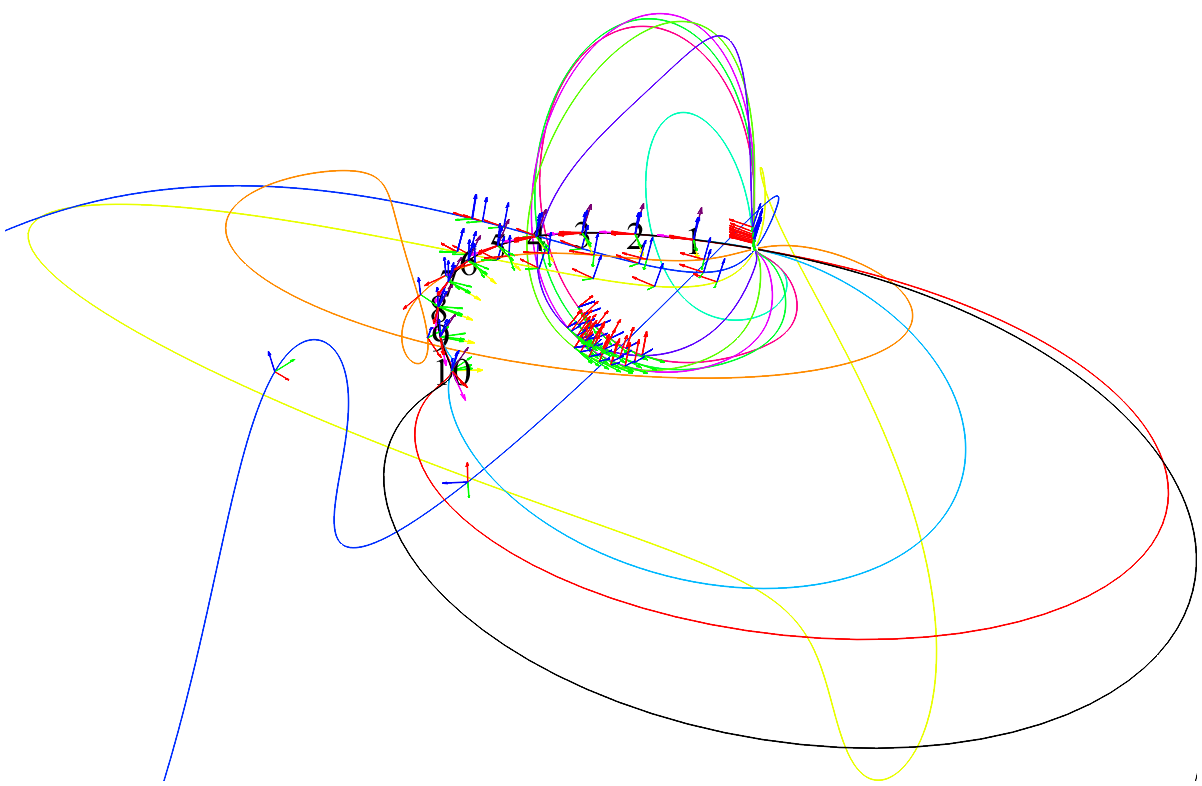
The evolution rule consists of comparing coordinates of the curve velocity (3) with respect to some orthonormal basis of with the coordinates of the difference vector from foot point to target point. This produces an overconstrained system which is solved in least square sense. Hence the shape parameters approximately change with the corresponding amount and the process is repeated again starting with the foot point computation. The final results are presented in Table 2 with a three decimal digit precision. The evolution process itself is visualized in Figure 1. The target poses are labelled from 1 to 10, the angles and distances to the respective target poses are given in Table 3. It can be seen that the distances are quite good while the orientation seems to be hard to match. The reasons for this are under investigation. We conjecture an inappropriate distribution of feature points.

| TP s | TP1 | TP2 | TP3 | TP4 | TP5 | TP6 | TP7 | TP8 | TP9 | TP10 |
|---|---|---|---|---|---|---|---|---|---|---|
| t |
After the motion curve is obtained we can start the synthesis of the overconstrained 6R linkage using motion factorization [4] as explained in Section 2. First the quadratic factors are computed by multiplying the curve with it’s quaternion conjugate:
| (7) |
By selecting the first quadratic factor from (7) polynomial division (a variant of Euclid’s algorithm taking into account the non-commutativity of quaternion multiplication) is used to divide and single out the remainder
| (8) | ||||
The constant term in the rightmost factor is computed as a unique root of this linear remainder polynomial:
| (9) |
After the first root is computed , is divided by and the process is iterated with the quotient and with one of the remaining quadratic factors from (7). After the second root is computed the quotient will be the last linear factor. All the possible combinations in which the quadratic factor can be chosen will produce six different open 3R kinematic chains. Suitable combinations [4] then give overconstrained 6R linkages. Four examples are depicted in Figure 2


5 Conclusions
We used properties of the factorized representation of rational motions to set-up an evolution process for optimal design of corresponding linkages. The evolution gives an open kinematic chain that, if desired, can be combined with other chains obtained from different factorizations to produce overconstrained linkages. From a mechanical point of view, overconstrained linkages are robust, need minimal control elements and they are ideal for repetitive motions in an interval. In Section 4 we illustrated this process for an overconstrained 6R linkage. So far, position matching is good while matching orientations should be improved.
The construction relies on the factorized representation which helps to ensure validity of the Study condition throughout the evolution and automatically relates the rational motion to kinematic chains. Moreover, rationality allows efficient and stable computation of footpoints which is a crucial part in any evolution based mechanism synthesis.
The research was supported by the Austrian Science Fund (FWF): P 26607 (Algebraic Methods in Kinematics: Motion Factorisation and Bond Theory).
References
- [1] Aigner M., Šír Z. and Jüttler B.: Evolution-based least-squares fitting using Pythagorean hodograph spline curves. Computer Aided Geometric Design, 24:6 310–322 (2007)
- [2] Aigner M. and Jüttler B.: Hybrid curve fitting. Computing 79:2 237–247 (2007)
- [3] Cabrera, J. A. Simon, A. and Prado, M.: Optimal synthesis pf mechanisms with genetic algorithms. Mechanism and Machine Theory, 37:10 1165–1177 (2002)
- [4] Hegedüs G., Schicho J., and Schröcker H.-P.: Factorization of rational curves in the Study quadric and revolute linkages. Mechanism and Machine Theory, 69(2), 142–152 (2013)
- [5] Hegedüs G., Schicho J., and Schröcker H.-P.: Four-Pose Synthesis of Angle-Symmetric 6R Linkages. Journal of Mechanisms and Robotics 7:4 50–57 (2015)
- [6] Hofer M., Pottmann H.: Energy-Minimizing Splines in Manifolds. Transactions on Graphics 23:3, Proceedings of ACM SIGGRAPH 2004 284-293 (2004)
- [7] Hofer M., Pottmann H., and Ravani B.,: From curve design algorithms to the design of rigid body motions. The Visual Computer 20:5 279–297 (2004)
- [8] Hofer M., Pottmann H. and Ravani B.: Geometric design of motions constrained by a contacting surface pair. Computer Aided Geometric Design, 20:8 523–-547 (2003)
- [9] Husty M. L., Schröcker, H.-P.: Algebraic Geometry and Kinematics. In book: Nonlinear Computational Geometry, pp 85-107 (2009)
- [10] Larochelle P.M., Murray A.P. and Angeles J.: SVD and PD based projection metrics on SE(n). In: On Advances in Robot Kinematics, ed. by Lenarčič, J. and Galetti, C. Dordrecht, Boston and London: Kluwer Academic Publishers, pp. 13-22 (2004)
- [11] Paradis M. J. and Willmert K. D.: Optimal Mechanism Design Using the Gauss Constrained Method. J. Mech., Trans., and Automation, 105(2), 187–196 (1983)
- [12] Schröcker, H.-P. Jüttler, B. and Aigner M.: Evolving Four-Bars for Optimal Synthesis. In: Proceedings of EUCOMES 08, The Second European Conference on Mechanism Science, pp. 109-116 (2009)
- [13] Zhang, X. Zhou, J. and Ye, Y.: Optimal mechanism design using interior-point methods. Mechanism and Machine Theory, 31:1, 83–98 (2000)