Entrainment induced by waves at a density interface impinged by a turbulent jet
Abstract
Using water/salty-water laboratory experiments, we investigate the mechanism of erosion by a turbulent jet impinging on a density interface, for moderate Reynolds and Froude numbers. Contrary to previous models involving baroclinic instabilities, we show that the entrainment is driven by interfacial gravity waves, which break and induce mixing. The waves are generated by the turbulent fluctuations of the jet and are amplified by a mechanism of wave-induced stress. Based on the physical observations, we introduce a scaling model which varies continuously from the to the power law from small to large Froude numbers, in agreement with some of the previous laboratory data.
keywords
1 Introduction
Turbulent mixing in stratified flows is found in many geophysical and industrial situations and relies on a complex process where the kinetic energy is irreversibly converted into potential energy (Fernando, 1991; Fernando & Hunt, 1996). The present paper considers the case of a sharp density interface impinged by a turbulent round jet. The turbulent jet of light fluid (water) of density impinges on a volume of denser fluid (salty water) of density , such that the outflow of the jet is orientated in the gravity direction and orthogonal to the density interface. The jet is driven by an upstream pump. The salty water is progressively mixed with the fresh water until the gradients of density disappear. In this process, two mechanisms can be identified: the entrainment and the mixing. The entrainment corresponds to the advection at the interface of dense fluid patches into the lighter fluid, where the flow is turbulent. The mixing consists in the thinning of the fluid patches by the turbulence until the spatial scale reaches the molecular diffusion scale, where both fluids are irreversibly mixed. The turbulent entrainment is quantified by the entrainment rate (Baines, 1975)
| (1) |
where refers to the volumetric flux entrained across the interface and and correspond to the vertical velocity and the width of the jet at the interface. Baines (1975) suggested that for a turbulent flow, the entrainment rate depends only on the interfacial Froude number, where the Froude number is with the reduced gravity acceleration. The Froude number characterizes the competition between the inertial force, which perturbs the interface, versus the restoring buoyancy force. Since Baines (1975), the entrainment flux has been commonly expressed as a power-law function of with and .
The significant scatter in measurements of the entrainment rate has been summarized by a recent review of Shrinivas & Hunt (2014) for jet, plumes and fountains. They report the entrainment rates of different studies (Baines, 1975; Kumagai, 1984; Baines et al., 1993; Lin & Linden, 2005) and show that at low Froude number, two distinct trends are observed. The measurements of Linden (1973), Baines et al. (1993) and Lin & Linden (2005) for fountains and Baines (1975) for plumes follow approximatively the scaling law for . The measurements of Kumagai (1984) for a plume display a distinct branch with larger entrainment rates. Kumagai (1984) originally characterized the scaling law by but Shrinivas & Hunt (2014) propose the scaling law . Cotel et al. (1997) have also studied the entrainment rate for an impinging jet. They observed two different behaviours: a linear scaling with for , which decays to a constant for . A universal law for the entrainment rate as a function of the solely Froude number seems to be ruled out by the previous experimental investigations, which suggest that other parameters must be taken into account.
Breidenthal (1992) and Cotel & Breidenthal (1996) proposed to characterize the regimes with the Reynolds numbers , where is the kinematic viscosity, in addition to the Froude number. Baines (1975) showed that the entrainment rate does not depend on the Reynolds number providing the flow is turbulent. However, Shy (1995) observed that the properties of the flows inside the impinged region change drastically when the Reynolds number is increased. For moderate Reynolds number (), the density interface in the impinged region remains sharp with a small mixed layer thickness but above , the thickness of the density gradient increases by a factor : it is the so-called mixing transition. Shy (1995) interpreted this transition as a strong enhancement of baroclinic turbulence inside the dome. Cotel et al. (1997) verified the presence of this transition, but the authors confirmed the experiments of Baines (1975) by showing that remains independent of the Reynolds number for . The problem of how the phenomenology differs at the transition without modifying is still open.
Describing the turbulent flow as a superposition of vortices, the models of erosion are commonly based on the mixing capacity of vortices, determined by their Froude number , with radius and velocity (Linden, 1973; Shy, 1995; Cotel et al., 1997; Cotel & Breidenthal, 1996). Only the vortices with are expected to contribute significantly to the entrainment in the impinging region. The classical model of engulfment of Linden (1973) states that the eddies rebounding on the interface engulf the dense fluid before being advected by the mean flow outside the dome. Linden (1973) proposes a law based on scaling arguments and kinetic and potential energy balance. Shy (1995) and Cotel et al. (1997) report the presence of persistent baroclinic vortices localised around the periphery of the dome. The baroclinic vortices are generated by the incident small scales vortices advected by the turbulent jet. From these qualitative observations, Shrinivas & Hunt (2014) suggest a mechanism of entrainment based on a stationary circulation driven by like-sign vortices forced by baroclinic effects. For the low Froude number regime, it leads to a scaling in unconfined geometries. In confined geometries, Shrinivas & Hunt (2015) suggest that the presence of large scale oscillations of the interface leads to a correction , so that the entrainment rate becomes , with a constant vanishing in the unconfined limit. They show that the confinement effect may explain the scatter of the data observed in their graphics, i.e. the existence of two branches at low Froude number.
The model of Shrinivas & Hunt (2015) attempts to rationalise the different entrainment laws but it relies on the presence of vortices driven by baroclinic forces, even if no experimental study has demonstrated quantitatively their existence. The presence of the mixing transition suggests that the strength of the baroclinic vortices inside the dome depends on the Reynolds number of the turbulent jet. Turbulence in jets with large Reynolds numbers () is expected to be developed and to display small scales structures, more efficient to generate baroclinic (Shy, 1995), whereas jets with moderate Reynolds numbers () remain dominated by large scale structures (Dimotakis, 2000). These points raise two questions: can the vortices of a turbulent jet drive baroclinic eddies for Reynolds numbers below the mixing transition? What is the mechanism of entrainment at moderate Reynolds numbers if the baroclinic vortices are absent? These questions will be addressed here.
In the present paper, we aim at determining the mechanism of entrainment of a non-buoyant jet impinging a sharp density interface via velocity and density measurements for Reynolds numbers below the mixing transition. Our experimental set-up is presented in section 2 and 3. Our study holds for moderate , i.e. , corresponding to a relatively small deformation of the interface, and for moderate Reynolds numbers (). Our measurements support a mechanism where the entrainment is driven by interfacial gravity-waves as shown in section 4. The waves are generated by incident vortices and amplified during their propagation outside the impinged region. This amplification leads to wave breaking associated with local mixing. Based on our measurements and on this mechanism, we introduce in section 5 a model describing the continuous change of the scaling law for turbulent entrainment from small to large Froude number.
2 Experimental set-up
2.1 Set-up and measurements
The set-up is sketched in figure 1(a). The tank is rectangular with a square section of width cm and height H cm. The tank is filled with one layer of light fluid of density and height cm above a layer of denser fluid of density and height cm (figure 1). The densities are controlled by a density meter DMA 35 from Anton Paar. The upper part of the tank is filled with water, plus some ethanol for the experiments indexed by M, M and M in table 1. The lower part of the tank is filled with a saline solution of density . The solution of ethanol in the light fluid allows us to match the optical index of the saline solution below. The viscosity of the mixture water plus ethanol is a non-linear function of the percentage of ethanol. The index matching is performed for density jump . The measurements are performed with an initial density , which is associated with a kinematic viscosity of at K (Khattab et al., 2012). The initial viscosity is larger than the viscosity of the water but the mixing will progressively decrease this difference during the run. All the fluids are freshly prepared for each run and filtered (20 microns filter). The velocity of injection at the round nozzle of radius cm is fixed for each experiment. The pump for the injection is located in one of the upper corner of the tank: the experiments are thus performed with a constant volume. Our measurements shows that the pumping system does not modify significantly the symmetries and properties of the mean velocity field.
(a) (b)

| Run | ||||||||
|---|---|---|---|---|---|---|---|---|
| T1 | 1.15 | |||||||
| M1 | 1.03 | 0.031 | 41.8 | |||||
| M2 | 1.15 | 0.031 | 46.6 | |||||
| M3 | 1.15 | 0.028 | 49.1 |
Two different experimental investigations are performed: the first one for the description of the turbulent jet without density variation, and the second one for the investigation of the mixing mechanism. The runs are respectively indexed by “T“ and “M“(table 1). The physical properties of the waves (section 4.2) and the features of the breaking (section 4.5) are determined from the measurements of the density field, run indexed by M2. The excitation (section 4.3) and the amplification (section 4.4) of the waves are mostly characterized by the velocity measurements in runs indexed M1 and M3. We have checked that the runs display the same features, like the signature of the wave period in the measurements of density M2 (figure 9) and in the measurements of velocity M1 (figure 11(a)). The measurements start four minutes after the beginning of the erosion. We performed both velocity and density measurements using a digital camera (FASTCAM Mini, Photron) with a spatial resolution of pixels.
The velocity field is measured in the experiments T1, M1 and M3, using the particle image velocimetry (PIV) process (Meunier & Leweke, 2003). The flow is seeded with tracer particles () and it is illuminated by a laser sheet crossing the vertical plane of the jet. The dimensions of the interrogation windows are cm2. The acquisition rate is performed at fps and frames are acquired. The PIV algorithm is based on a first pixels and a second pixels interrogation regions, and the resulting velocity field is a vector field. The convergence of the mean field is insured for an ensemble of frames larger than snapshots. During the PIV measurements, the interface between the fluids is detected independently via a small amount of rhodamine in the dense fluid. In the experiment M2, the density is measured by a planar laser-induced fluorescence technique (PLIF) with the same laser and camera set-up. The saline solution is mixed with rhodamine B. This rhodamine has an absorption spectrum between 460 and 590 nm and its emission spectrum is 550-680 nm, well separated from the laser light. A high-pass filter (TIFFEN Filer, orange 21) is mounted on the camera with a cut off frequency of 550nm. The calibration has been performed with uniform fields of density. The dye concentration has been adjusted to have a linear relation between dye concentration and intensity. From this calibration process, we have calculated the measured spatial intensity distribution, called also flat-field, which takes into account the biased of intensity due to the lighting inhomogeneity or the camera response. The density of rhodamine is then calculated from the intensity field corrected by the flat-field. Here, we are only interested in iso-density contours defining the interface. We define the interface height as the curve of iso-density .
The initial distance between the end of the nozzle and the interface is cm (runs , see table 1) , i.e. times the diameter of the nozzle in order to obtain a developed turbulent jet (List, 1982). To describe the flow, we use the frame in the plane of symmetry of the jet (figure 1(b)) with the cartesian coordinate system . The -axis is aligned with the radial direction and the -axis corresponds to the axis of symmetry of the jet. The origin is located at the nozzle outlet. Due to the axisymmetry of the configuration, we assume that the time-averaged quantity of the azimuthal component of the velocity fields, here in the direction, and the derivative of the average quantities with respect to , are equal to zero. The measurements performed in the vicinity of the impinged region are expressed as a function of the radial distance and the distance from the interface , where is the time average distance from the nozzle to the interface along the axis of the jet.
2.2 Interfacial dimensionless parameters
In table 1, we report the Froude numbers and the Reynolds numbers associated with the jet for each run: and . The Reynolds number is expected to be constant in the far field of the jet (List, 1982). The Reynolds numbers are between and , which implies that our experiments are below the mixing transition (Shy, 1995), where the mixing layer thickness is small. We investigate the properties of the solely turbulent jet configuration in the next section. From the Froude numbers , we calculate a relevant Froude number at the interface by interpolating the typical length and velocity at the interface. We use the classical law of evolution of the width of the jet and the axial velocity component with a distance from the nozzle (Fischer et al., 1979)
| (2) |
with the spreading rate, the velocity decay constant and the virtual origin of the jet reported in table 2. We use the top-hat definition for the typical length and velocity . The top-hat definition for a gaussian profile allows us to define and with the position of the interface. The recent numerical experiment of Ezhova et al. (2016) supports the use of equations (2) showing that the axial velocity component (Fig.6(a)) is modified only in the near field of the interface. The Froude number at the interface
| (3) |
writes as a function of the position of the interface
| (4) |
Thus the Froude number decreases like . Our study is performed during a limited duration after the initial transient and, it is reasonable to consider that the Froude number has not varied significantly since the beginning of the experiment.
| [cm] | ||||||
|---|---|---|---|---|---|---|
| T1 | ||||||
| Hussein et al. (1994) |
3 Kinematics of the jet
3.1 Jet without stratification
(a) (b)


We first study the jet in the absence of stratification for a Reynolds number (T1 in table 1) in order to validate the use of equation (2). The measurements are performed for between and . The local radius of the jet divided by the diameter is reported as a function of in figure 2(a). The radius corresponds to the ordinate where the average vertical velocity corresponds to the half of the axial velocity, i.e. , for a given . The radius increases linearly and the fitted parameters (equation (2)) are reported in table 2. The ratio (figure 2(b)) increases also linearly and the corresponding parameter is reported in table 2. The coefficient is fitted by taking as a function of with obtained from the data of figure 2(a). The measured coefficients are compared to the results of Hussein et al. (1994) for , based on the radius of the nozzle. Our measurements are in good agreement, regarding and , which are related to the physics of the mixing by the turbulent jet: this validates the use of Taylor entrainment constant. The virtual origin is different but it depends strongly on the range of fitting , as demonstrated by Wygnanski & Fiedler (1969).
3.2 Jet with stratification
We now focus on the velocity field of a jet impinging on a sharp density interface. The results presented here correspond to the run M1 (table 1). The vertical component of the time-averaged velocity field and its streamlines are reported on figure 3. The operator corresponds to the time-averaged quantities calculated on a duration s corresponding approximatively to advection time scales . The white curve represents the time-averaged location of the interface determined by the presence of fluorescent rhodamine. The vertical axis at corresponds to the jet axis and the height is associated with the bottom of the time-averaged interface (black dashed line).
We have reported in table 1, the depth and the radius of the time-averaged dome generated by the impact of the jet on the stratified interface for M1, M2 and M3. The radius is the radial distance between the center of the dome (almost parabolic) and the end of the dome, where the interface becomes flat. The depth corresponds to the difference of altitude between these two extremities. For M1, the dome is characterized by a radius cm and a depth cm. The abscissa and the height will be rescaled respectively by and in the rest of the paper. The radius of the jet at the interface , equal to cm, corresponds approximately to the width of the jet entering in the dome and it is approximatively two times smaller than the radius of the dome.

(a) (b)


A remarkable property of the flow inside the dome is the convergence of the streamlines leaving the dome close to the interface. This contraction corresponds to a local acceleration of the flow. To study the flow field inside the dome, we introduce the velocity component , which is tangential to the mean interface given by the function . For each abscissa , we calculate the angle of inclination of the interface given by and we define the velocity by . The profiles of are reported in figure 4(b) for different abscissae shown in figure 4(a)(from left to right) starting at cm () and finishing at cm (). They are plotted as a function of the ordinate following the normal to the interface (dashed lines in figure 4(a)) with the interface at . The curves correspond to the polynomial interpolation of the profiles. The profiles confirm that the flow accelerates along the interface.
A balance between potential energy and kinetic energy explains the acceleration characterized by . When the jet impacts the interface, the kinetic energy is converted partially into potential energy. When the flow leaves the dome, a part of the potential energy is reconverted into kinetic energy. We have calculated the kinetic energy as a function of the height along the interface (figure 5(a)). The kinetic energy increases initially linearly with the height until , which corresponds to the abscissae . The time-averaged interface follows the streamline of the time-averaged flow passing close to the stagnation point at . Shrinivas & Hunt (2014) (equation (3.9)) suggest that despite the presence of turbulence, the Bernoulli equation can be applied along the streamline following the interface. By assuming a pressure balance at the interface and a vanishing velocity below the interface, they obtain . However, our measurements show that the kinetic energy follows : only six percent of the potential energy is transferred into kinetic energy. The application of the Bernoulli equation breaks because the velocity does not vanish rapidly below the interface (figure 4(b)) and it considers neither the process of entrainment nor the turbulent fluctuations, which must consume an important part of the potential energy. Outside the dome, the streamlines are directed upward and reconnect the jet flow drawing a large recirculation cell. This recirculation is the combination of the ballistic reflection of the jet and the lateral entrainment of the jet.
(a) (b)


4 Investigation of the mechanism of erosion
4.1 General description
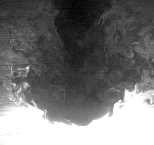
We first draw a global picture of the mechanism of erosion before demonstrating each element in the following paragraphs. When the jet impinges on the dense fluid, the interface is convoluted by the turbulent fluctuations of the jet. These perturbations are generated by eddies coming from the jet. These vortices excite interfacial gravity waves propagating outward the impinged region (figures 6). During the propagation, the height of the waves increases until they breakdown close to the border of the dome. This process is illustrated on the three successive pictures of the interface of figure 6(b), with waves propagating from left to right. The amplification of the waves is caused by an energy transfer from the mean flow via a mechanism, which could be similar to the one described by Miles (1960) in shear flows. The breaking of the waves induces a strong mixing due to the wrapping of filaments. The heavy fluid is then transported in the bulk flow where the turbulence of the jet mixes both fluids (figure 6(a)). We claim that the transport and the mixing of the dense fluid by these waves is the main source of erosion at low Froude number and moderate Reynolds numbers. The following sections detail successively the former points.
(a) (b)

4.2 Wave properties
In this section, we characterize the properties of the perturbations near the interface. We observe that the interface remains sharp in the impinged region, as expected for (Shy, 1995) with a small diffusion layer . The height of corresponds to few percent of the dome depth, i.e. few millimeters. The stratification in this layer could support internal gravity waves with typical frequency with the associated density gradient. The frequency of internal gravity waves would be Hz for mm. As we will see further, the typical frequency of the waves propagating inside the dome varies in the range Hz, a frequency range corresponding to interfacial gravity waves. Hence, the dynamics of the perturbation inside the dome is controlled by interfacial gravity wave rather than internal gravity wave.
The spatio-temporal properties of the waves is studied by using the information contained in the dynamics of the interface. The perturbation of the interface is illustrated by an instantaneous relative density field from the measurement M2 (figure 7). The relative density is defined by varying between and , with the effective density given by the LIF measurements. The interface position defined by (black curve) corresponds to the iso-density line . The time-averaged height is represented by a black dotted curve following a quadratic law in the impinged region.

From the height , we introduce the height perturbation and we perform a two-dimensional spectrum of the spatio-temporal evolution of . It consists in projecting the spatio-temporal field inside the dome, i.e , on the 2D Fourier space . We restrict the spatial domain to the dome region, where the waves are generated and amplified. We report in figure 8, the two-dimensional power-spectrum with frequencies below Hz and wavenumbers smaller or equal to , with (run M2, table 1). This bandwidth contains percent of the total energy. The temporal dynamic of the height is mostly modulated by two time-spectral components: slow standing modes and interfacial gravity waves. The slow mode is characterized by frequencies in the range with a peak in the mode with wavelength . The waves are characterized by wavenumbers between and , i.e wavelengths between and , and frequencies in the range , i.e a typical period with s. The energy in the waves is approximatively two times larger than the energy in the slow modes. The precise characterization of the wavelength is difficult because the wavelength is comparable with the length of propagation. The dispersion relation of interfacial waves for irrotationnal flow gives a period of , a value comparable to the measured one. The difference may be explained by the presence of an inclined interface of propagation or by the Doppler shift associated with a mean non-uniform flow.
By using a bandpass filter containing the frequency range Hz, we are able to extract the propagation of the interfacial waves. The spatio-temporal diagram of the bandpass filtered is reported on figure 9(a), with the abscissae rescaled by and the time by the period of the waves . The amplitude of the waves is divided by the depth of the dome . The spatio-temporal diagram displays wave patterns with a half-wavelength comparable to the dome radius. The wave dynamic is complex but we observe that most of the waves propagates outward the dome, as illustrated by the figure 9(b). From the bandpass filtered elevation , we perform a lagrangian tracking of the waves, which consists in following the wave envelop. We report some trajectories on figure 10(a) and calculate the phase velocity . The velocities being not constant, we calculate the probability density function of for all the trajectories (insert of figure 10(a)). The distribution exhibits a maximum at , which will be taken as the reference phase velocity at the interface. The grey dashed curve on figure 10(a) corresponds to a trajectory with .

(a) (b)


We also calculate the root mean square amplitude of the wave
| (5) |
with the height perturbation without the slow modes component suppressed by a high-pass filter and the duration of the measurement. We report (upper dotted curve, called total) as a function of on the figure 10(b). The dashed curve (called fundamental) corresponds to the amplitude of the waves in the frequency range Hz (by using a band-pass filter) and the heavy curve corresponds to the amplitude with higher frequencies. Despite the fact that the typical length scale of the waves is comparable with the distance of propagation, we distinguish different behaviors of the amplitude of the wave during the propagation. We have reported the three regions of interest: the region I, where the waves are generated and amplified; the region II, where the waves break, and the region III out of the dome. The amplitude of the fundamental frequency increases in the region I (), suddenly drops in the region II, and then decreases monotonically out of the dome . In the breaking region, the amplitude of the modes with large frequencies decreases just after those of the fundamentals. The shift of the amplitude drop is a consequence of the wave breaking, where the density patches are wrapped and thinned (figure 6(b)).
(a) (b)


4.3 Wave generation
We now focus on the waves excitation mechanism, with two possible candidates: the instability of the interface and the interface excitation by turbulent fluctuations. First, we investigate the stability of the interface and we demonstrate that the shear at the interface is not strong enough to trigger Kelvin-Helmholtz and Holmboe instabilities.
The stability of the interface is related to the local Richardson number given by with the shear defined by at and the frequency of interfacial gravity waves. It compares the destabilizing effect of the shear to the stabilizing buoyant effects. The perturbations being interfacial gravity waves, the Richardson number is defined by (Chandrasekhar, 1961). It is worth noting that by using the frequency of internal gravity waves instead of the one of interfacial waves, the Richardson number becomes one order of magnitude larger that the one defined here.
The shear is calculated from the mean velocity field and corresponds to the tangential velocity gradient at the interface (figure 4(b)). We have shown that the interface merges with a streamline of the average flow passing close to the stagnation point (figure 3). The mean velocity field along the interface satisfies the relation for , which implies that by considering the continuity of the mean material line. The average velocity field and the mean position of the interface may be considered in quasi-equilibrium, supporting the stability analysis of the interface from the mean fields.
The local Richardson number is reported on the figure 5(b). It varies between and in the vicinity of the head of the dome, i.e. or . It turns out that the interface should not be destabilized in this region by a classical Kelvin-Helmholtz instability operating for (Miles, 1961; Chandrasekhar, 1961)(see also the numerical simulations by Woodward et al. (2014) on a closely related problem). We point out that the presence of a curved interface and an accelerating flow, i.e , may change the criteria of stability. Nonetheless these effects are only significant on the sides of the dome, where the waves are already excited and amplified.
Moreover, the length scale of the instability is not compatible with the one of the Kelvin-Helmholtz instability. For a sharp velocity jump, the smallest unstable wave number is given by (Chandrasekhar, 1961)
| (6) |
with the velocity jump at the interface and the Atwood number. From figure 4(b), the largest velocity jump is typically cm/s inside the dome. The numerical application gives m -1 corresponding to a wavelength smaller than cm. The Kelvin-Helmholtz instability could only trigger perturbations at scales times smaller than the one observed. Reciprocally, the velocity jump should be at least times larger to account for the observed wavelength. During the erosion process, decreases (Kumagai, 1984): if the interface is initially stable for the Kelvin-Helmholtz instabilities, it remains so during the erosion process.
An other alternative to the Kelvin-Helmholtz instability is the Holmboe instability (Holmboe, 1962). This instability can operate for large Richardson numbers and Alexakis (2009) showed that it may appear for (far from the of the K-H instability). However, the Richardson number is larger than for in the dome. The mode associated with the Holmboe instability is also characterized by symmetric cusps at large Richardson number (Strang & Fernando, 2001). This pattern has not been observed in our experiment. We conclude that neither the Kelvin-Helmholtz instability nor the Holmboe instability generate perturbations on the interface.
(a) (b)


The source of waves is ensured by the turbulent fluctuations of the jet. Having identified the region and the frequency range of the waves in section 4.2, we look for their signature in the turbulent jet. In order to demonstrate that the perturbations come from the jet, we focus on the fluctuations of the vertical velocity fluctuation along the axis , represented by the dashed curve on figure 11(b). We calculate the bandpass filtered component of in the frequency range Hz. The associated spatio-temporal diagram is reported on the figure 11(a) with and rescaled by the period of the wave and the depth of the dome . We clearly identify perturbations propagating from the jet to the dome. It is worth noting that these fluctuations appear far from the dome at and seem to be incoherent before. This region is far from the transitional distance close to the nozzle of the jet (), where coherent structures may be generated in the early development of the jet (Yule, 1978). Thus, it is possible that a coherent process, based on the interplay between the jet and the interface, may filter or select the perturbations far from the interface. The bandpass filtered fluctuation of vorticity field, calculated from a coarse-grained velocity field, is reported on figure 11(b) for a given time . The fluctuations are associated with large scale vortices, which propagate toward the interface. The diameter of the vortices close to the dome is varying around cm. At the entrance of the dome, the typical vertical velocity is (figure 3). So a typical period of excitation corresponds to the advection of two vortices of opposite sign and the associated time scale of forcing is s, a value very close to the wave-period .
From the fluctuation , we can estimate a Richardson number for the observed eddies. The maximum amplitude of reaches typical value given by cm/s. The Richardson number of these eddies is defined by (Cotel & Breidenthal, 1996) and corresponds to . An energy balance between the kinetic energy of the vortex and the potential energy associated with the penetration depth gives (Linden, 1973). From the measured Richardson number, the penetration depth is of order . Thus the convolution of the interface is expected to be too small if we consider the classical model of the vortex impact. It has been recently demonstrated in the context of internal-gravity waves excited by turbulent plume that waves can be forced by the bulk pressure-field of the turbulence (Lecoanet et al., 2015). This approach could be fruitful to explain the wave excitation for eddies with low Richardson numbers.
4.4 Wave amplification
The observed growth of the perturbations along the interface (figure 10(b)) may be explained by a mechanism of wave amplification. Furthermore, the axisymmetry of the configuration leads a priori to a decrease of the energy of the perturbations, due to the radial spreading of the energy. Thus, the amplification must at least counterbalance the energy spreading due to the axisymmetry. As shown in the previous section, the amplification mechanism could not be explained by the Kelvin-Helmholtz and Holmboe instabilities. It is interesting to note that our configuration shows some similarities with the problem of the generation of ocean-waves by turbulent wind (Janssen, 2004). The ocean-waves are generated by turbulent pressure fluctuations with a sheared mean flow. Like in our configuration, the Kelvin-Helmholtz is not the best candidate to explain the generation of ocean-waves (Janssen, 2004). Focussing initially on an ideal configuration of a shear flow with a density jump (Miles, 1957), Miles (1960) showed that the presence of a shear flow may lead to an enhancement of the energy transfer to the waves in turbulent shear flows. This scenario is based on the presence of a critical layer (Miles, 1957) at the height where the phase velocity of the waves matches the velocity . It is usually called the Miles instability. The Miles instability permits the transfer of energy from the mean flow to the wave if at the critical height , the second derivative of is negative. This instability is characterized by waves induced stress, where the Reynolds stresses of the velocity fields are non-zero. A physical interpretation of the instability is given by Lighthill (1962). This mechanism is similar to the critical layer encountered in shear flow without inflection point (Drazin & Reid, 2004), but it differs from the critical layer found in stratified flows, where the internal gravity wave gives its energy to the mean flow, even if the amplitude of the wave may increase due to the wave-action conservation (Sutherland, 2010). Our measurements show that the mechanism of amplification operating in the dome shares some features with the Miles instability. Despite the difference in geometry between the framework of the Miles instability and our configuration, we use the theoretical result of the Miles instability, in the absence of theoretical prediction adapted to our case.
(a) (b)


First, we look for the region of resonance where the typical phase velocity and the tangential velocity are equal. In figure 12(a), the velocity is divided by the phase velocity for the half plane of symmetry of the jet given by . The white curve is the mean interface . The closed dashed curve represents the contour where : inside this region, the wave may propagate slower than the flow. The enclosed region appears for and ceases for . If the Miles instability is present, an increase of the disturbance energy must be seen through the action of the Reynolds stress (Lin, 1954; Drazin & Reid, 2004). The energy transfer between the mean flow and the waves is given by the production term , with the large scale shear and the Reynolds stress . The Miles instability must be associated with a positive production term in the region where . The production term is calculated for the run M (see table 1) and it is reported on figure 13. We observe that the production term is positive for larger than and it becomes negative for in between and , depending on the height. The transition between positive and negative production occurs in the region where for (dashed curve figure 12(a)), suggesting the presence of a critical layer. The production term is non-zero above the interface, as expected from the Miles instability. The sign of the shear remaining constant for each side of the dome ( for and for ), the variation of is associated with a change of sign of the Reynolds stress . It is a classical property of the critical layer (Miles, 1957; Drazin & Reid, 2004). The relative phase between and varies abruptly across the critical layer where , leading to a change of the sign of the production term (Lin, 1954). The sign of is also correlated to the variation of the height of the waves (figure 10(a)). The height of the wave increases when is positive and it decreases when becomes negative. From the production term and the kinetic energy of the wave , an estimation of the energy transfer rate of the wave is possible with . We report the maxima (heavy black line) and the minima (dashed black line) of the dimensionless energy transfer rate for all heights in the dome as a function of on figure 14. The positive energy transfer rate reaches the values at and the damping rate reaches the values for . We clearly observe that the waves are amplified, with , in the central region and they are significantly damped outside, with The grey lines correspond to the abscissa where the waves may propagate slower than the mean flow. Once again, the transition between amplification process and damping process occurs in the region where the waves cross the critical layer.
The calculation of the growth rate of the Miles instability is complex and an explicit formula exists only for idealized configurations (Miles, 1957; Morland & Saffman, 1993; Drazin & Reid, 2004). The growth rate depends on properties of the mean flow at the critical layer and its calculation requires the knowledge of the amplitude of the initial neutral perturbation. It is out of reach of the present study and we will only focus on the sign of the growth rate in order to confirm the presence of the instability. The grow rate is given at leading order in (Miles, 1957; Drazin & Reid, 2004; Young & Wolfe, 2014)
| (7) |
with the ratio of the streamfunction at the critical layer, which is especially difficult to estimate. Considering wave-amplification, the growth rate may be interpreted as a energy transfer rate from the mean flow to the waves (Miles, 1960). The criteria of instability requires that the second derivative of must be negative. In figure 4(b), the profiles of are concave, which suggests that is negative. We verify this properties for the profile at (fifth profile starting from the left of figure 4), where for equal to and cm. The first derivative and the second derivative are reported on figure 12(b). The derivative remains negative in the region where the wave can be in resonance with the mean flow. The derivative is positive for cm. The sign of the ratio being negative, the mechanism of the Miles instability may amplify the wave. Our result shows that the amplification mechanism shares features with the Miles instability, suggesting the presence of a critical layer, that amplifies the waves generated by the eddies from the jet.

We have shown in the previous section that the waves are generated by the eddies of the jet and not by an instability. It could seem contradictory to the present section, which aims to demonstrate the presence of an instability. However, both mechanisms are complementary: the turbulence excites the waves and the instability amplifies them. It is a scenario similar to the ocean-wave generation mechanism. The opposite scenario may be addressed, i.e the waves are triggered by the instability and amplified by the turbulence. However, it is not very likely that the Miles instability may trigger a wave on a distance comparable to the half-wavelength. For the last point, Phillips (1957) has considered the wave-amplification by a resonance between the turbulent pressure field and the waves. By taking into account the presence of a critical layer, Miles (1960) has shown that this process is strongly enhanced by the Miles instability. Thus, once the wave is triggered, the energy transfer from the mean flow should be significantly larger than the energy coming from the turbulent fluctuations.

4.5 Wave breaking
We now focus on the wave breaking occurring in the region . In this area, different elements may explain the wave breaking. First, we have shown that when the phase velocity becomes larger than the mean velocity, the negative Reynolds stress damps the wave due to the critical layer. Then, the profile of becomes much steeper for (figure 4(b)). The associated local Richardson numbers (insert in figure 5(b)) are of order unity in this region, which may lead to a destabilization of the wave by a shear-instability. Finally, the steepness of the wave, which is defined by the product of the wavenumber with the height , becomes close to the critical steepness of the wave (Babanin, 2011). We consider the maximum average height of the wave (dotted curve indexed by total, figure 10(a)), which reaches the values with cm, i.e cm, for the run M (table 1). The maximum steepness based on the smallest wavenumber , where (run M2, see tab.1), is , a value in the range of wave-breaking criteria for ocean-waves (Babanin, 2011). The damping, the shear and the large steepness of the wave may lead to the wave breaking. It is difficult to disentangle the different effects, which can of course interplay between each others (Banner & Song, 2002).
After the breaking region just above the interface (figure 7(a) for cm and cm), we observe an area of mixed fluid with a relative density varying between and . It shows that the breaking has already induced mixing. Indeed, wave-breaking is believed to be the main mechanism of mixing at low Froude number (Fernando, 1991; Fernando & Hunt, 1996). The mixed fluid is then transported upstream, following the streamlines of the mean flow (figure 3). Figure 6(a) shows that the mixing continues at the frontier of the jet, where the turbulent intensity is expected to be important (List, 1982). Due to the lateral entrainment of the jet (section 3.2), a part of the mixed fluid is directly injected inside the turbulent jet.
4.6 Remark on the length and time scales
We have studied the different properties of the generation, the amplification and the breaking of the waves in the previous sections. These different mechanisms take place on a distance, i.e. the width of the dome, comparable to the wavelength of the wave. In the framework of the Miles instability, the long-wavelength perturbations are the most unstable (Miles, 1957; Morland & Saffman, 1993; Drazin & Reid, 2004). This mechanism could explain the observed large wavelengths in our confined geometry. From the lagragian point of view, the waves are generated and destroyed on time scales comparable to their period of oscillation. Figure 14 confirms that the evaluated energy transfer rate between the waves and the mean flow is close to the frequency of the wave. Unlike classical studies of waves propagation, the times and length scales are not well decoupled, which is a limitation of the local study of the stability of the interface.
Our study shows that the wavelength, the frequency and the growth-rate of the waves are determined by the forcing and the amplification mechanisms. In section 4.4, we have shown that both mechanisms are not independent: the perturbations propagating toward the dome oscillate at the wave frequency. A possible explanation is the existence of a global mode, coupling the dynamics of the interface and the flow outside the dome. The limitation of our local study may be due to the interpretation of a global mode in term of local perturbations. More work is needed for the theoretical analysis of the observed results, but we think the basic physical processes are correctly described here.
5 A scaling law for the entrainment rate
5.1 The scaling law
In the previous sections, we have demonstrated that the erosion is related to the dynamics of gravity interfacial waves. We want to address in this section the scaling law for the erosion rate, given by equation 1, as a function of the Froude number based on our observations. Linden (1973), Cotel & Breidenthal (1996) and Shrinivas & Hunt (2014) have suggested different physical arguments for the scaling law, leading to for the two first authors and for the later authors for . These models have not considered mechanisms involving waves for the erosion process, except for a footnote (page 476) in Linden (1973) from Dr E. J. Hinch. Based on the data of Baines (1975) and Baines et al. (1993), the entrainment rate should follow a scaling law at low Froude number and a linear scaling law at large Froude number. The volumetric flux entrained across the interface (equation 1) varies with the vertical entrainment velocity defined as the amount of fluid entrained per unit height per unit time (Linden, 1973). The entrainment rate, defined in equation (1), varies with the ratio (Cotel & Breidenthal, 1996)
| (8) |
where and are typical length and time associated with the erosion process and the vertical velocity of the interface. As we consider waves amplified by an unstable mechanism, is related to the relative length over which the amplification takes place, and to the frequency of the wave-perturbation. We have shown that the waves are triggered by the eddies in the jet with time scale comparable to the buoyancy frequency, i.e. . We choose the length as the distance travelled by the wave inside the dome minus the dome radius, i.e. (see fig.15(a)).
The waves exchange energy with the mean flow during the propagation along the distance (section 4.4). Hence, all the steps leading to the breaking of the waves take place on this distance. The length corresponds to a “useful“ length in the sense that for , no distortion and no erosion are expected in our model. This mathematical regularisation prevents the divergence of for , a regime not considered here. Cotel et al. (1997) report a constant erosion rate for , when the interface is almost flat. Our model quantifies the departure from this regime. Thus, we construct the length , so that it corresponds to the additional length travelled by the wave, when the dome is deepening for a constant dome radius . The infinitesimal length travelled by the wave on a interval is (figure 15(a)) and the useful length is
| (9) |
(a) (b)


with the depth of the dome as a function of . Our measurements show that , with the depth of the dome. By using the change of variable , the integral becomes
| (10) |
with . The integration gives
| (11) |
with the inverse of the hyperbolic sinus. We assume that the dome radius varies linearly with the radius of the jet . An energy balance between the kinetic energy of mean flow and the potential energy stored in the dome shows that , confirmed by the measurements of Shy (1995). For low Froude number , tends to zero and the length follows the asymptotic
| (12) |
The model shows that the length tends to for . At large Froude number with , we obtain
| (13) |
The two asymptotic behaviours are given by the function
| (14) |
Finally, the entrainment rate is given by
| (15) |
hence
| (16) |
Our model recovers both asymptotic behaviours as a function of the Froude number (figure 15(b)). We define the parametrization of the entrainment rate
| (17) |
with two real constants. The coefficient characterizes the crossover point , where the scaling law varies from to .
We now compare our model to the entrainment rate obtained in different processes of erosion (buoyant jets and plumes). We use figure 12(a) from Shrinivas & Hunt (2014) containing the measurements of Baines (1975) (triangles), Kumagai (1984) (squares), Baines et al. (1993) (crosses) and Lin & Linden (2005) (circles). We have reported the curve defined by equation (17) with in figure 16 (dotted curve). These parameters are determined by the best fitting of the experimental points of Baines (1975) (triangles), Baines et al. (1993) (crosses) and Lin & Linden (2005) (circles). The value of the coefficient defines the crossover point occuring at . The agreement is good between the theory and the experimental data. To conclude, our model requires only one fitting amplitude parameter, here , to fit the data both at low and large Froude number, once we have fixed the crossover point (given by ), unlike former models which require one parameter for each range.

5.2 Data of Kumagai
In figure 16, the data of Kumagai (1984) (upper branch) display a different trend relatively to the measurements of Baines (1975), Baines et al. (1993) and Lin & Linden (2005) (lower branch). The entrainment rate is approximatively one order of magnitude larger than the other measurements. The exponent of the scaling law has been debated for small Froude numbers: Kumagai (1984) initially proposed (dashed curve, figure 17), whereas Cardoso & Woods (1993) and Shrinivas & Hunt (2014) suggested (dotted line, figure 17). The data being scattered, both models seem valid. Hence, the existence of the upper branch may be interpreted in two different ways. If is equal to , two different physical mechanisms operate between the lower and the upper branch, as suggested in Shrinivas & Hunt (2015). If is equal to , the mechanism is unchanged but the pre-factors in the equation (17), and , vary with the conditions of the experiments, for instance because of confinement.

The data of Kumagai (1984) suggest that the transition between the behaviour at small and large Froude number occurs earlier compared to the lower branch. We have reported some values of the entrainment rate as a function of the Froude number (black squares) from figure 12 of Kumagai (1984) in figure 17. We observe a transition around in the upper branch (figure 17) whereas the lower branch is characterized by (figure 16). We recall that the coefficient in equation (17) determines the value of the transition . Hence, the entrainment rates measured by Kumagai (1984) may differ from the ones of the lower branch because and are different. Three models are reported in figure 17: the dashed curve corresponds to the empirical model of Kumagai (1984), the dotted line is the scaling law from Shrinivas & Hunt (2014) and the heavy black curve is given by the equation (17) with with a crossover point at . Our model follows the model of Kumagai (1984) up to . Once again, the set of data is not sufficient to determine which model is the best, even if we recover the empirical model of Kumagai (1984). However, our model shows that one possible origin of the upper branch is a modification of the pre-factors between the experiments.
Our model is based on the deformation of the interface and when the interface is weakly deformed, the entrainment rate follows a scaling law for . The coefficient determines the transition between a weakly deformed interface, when the width of the dome is larger than its depth, and a strongly deformed interface, when the width is significantly smaller than the depth. This transition should depend on the confinement, but also on the nature of the jet (buoyant or not) or the time-dependence of the erosion. Hence, the scatter of the measurements may be explained by a modification of the pre-factors , where characterizes the efficiency of the plume to deform the interface. But again, the physics of the erosion, dominated by breaking interfacial waves excited by the turbulent fluctuations and amplified by the mean flow, may remain the same.
6 Conclusion
In the present paper, we have investigated the mechanism of entrainment by a turbulent jet impinging on a density interface with moderate Reynolds number and moderate Froude number. In this regime, the vortices coming from the jet are not able to deform significantly the interface via ballistic impacts, as commonly expected by previous model involving baroclinic turbulence inside the dome. Their role is reduced to trigger interfacial gravity waves. The main source of energy comes from the mean flow, which amplifies the perturbation of the interface by a mechanism of wave-induced stress. The sign of the Reynolds stress changes abruptly inside the dome, where the phase velocity of the wave and the mean velocity field are equal. These features suggest the presence of a resonance between the wave and the mean flow. Wave amplification leads to wave-breaking in the vicinity of the border of the impinged region. The induced mixing is responsible for the irreversible erosion of the interface.
Based on these physical observations, we have introduced a scaling law, which varies continuously from the to the power law from small to large Froude numbers, in agreement with some of previous experimental measurements. Our model offers an alternative to Shrinivas & Hunt (2015): we suggest that the scatter of the measurements of the entrainment rate is rather due to a difference between the pre-factors of the scaling law rather than a modification of the exponents.
Our measurements are performed for Reynolds numbers below the mixing transition, i.e. . It will be interesting to investigate the mechanism of erosion at low Froude number and larger Reynolds numbers (), in order to verify if the present mechanism still operates or if others processes occur. For larger Reynolds numbers, the vortices impinging the stratification may be able to generate baroclinic vortices and turbulence at the interface, as suggested by Shy (1995). The model based on baroclinic effect, introduced by Shrinivas & Hunt (2014) and Shrinivas & Hunt (2015), could be then relevant.
Acknowledgements
The authors thank three anonymous referees for their comments and F. Duval (LIE, IRSN) and J.M. Ricaud (LIE, IRSN) for stimulating discussions. They acknowledge the support from the Institut de Radioprotection et de Sûreté Nucléaire and region PACA (France) under the APEX program 2015 (Project S2URF).
References
- Alexakis (2009) Alexakis, A. 2009 Stratified shear flow instabilities at large Richardson numbers. Physics of Fluids 21 (5), 054108.
- Babanin (2011) Babanin, A. 2011 Breaking and dissipation of ocean surface waves. Cambridge University Press.
- Baines (1975) Baines, W. D. 1975 Entrainment by a plume or jet at a density interface. Journal of Fluid Mechanics 68 (02), 309–320.
- Baines et al. (1993) Baines, W. D., Corriveau, A. F. & Reedman, T. J. 1993 Turbulent fountains in a closed chamber. Journal of Fluid Mechanics 255, 621–646.
- Banner & Song (2002) Banner, M. L. & Song, J. B. 2002 On determining the onset and strength of breaking for deep water waves. part II: Influence of wind forcing and surface shear. Journal of Physical Oceanography 32 (9), 2559–2570.
- Breidenthal (1992) Breidenthal, R. E 1992 Entrainment at thin stratified interfaces: The effects of Schmidt, Richardson, and Reynolds numbers. Physics of Fluids 4 (10), 2141–2144.
- Cardoso & Woods (1993) Cardoso, S. S. S. & Woods, A. W. 1993 Mixing by a turbulent plume in a confined stratified region. Journal of Fluid Mechanics 250, 277–305.
- Chandrasekhar (1961) Chandrasekhar, S. 1961 Hydrodynamic and Hydromagnetic Stability. Dover Publications.
- Cotel & Breidenthal (1996) Cotel, A. J. & Breidenthal, R. E. 1996 A model of stratified entrainment using vortex persistence. Applied Scientific Research 57 (3-4), 349–366.
- Cotel et al. (1997) Cotel, A. J., Gjestvang, J. A., Ramkhelawan, N. N. & Breidenthal, R. E. 1997 Laboratory experiments of a jet impinging on a stratified interface. Experiments in Fluids 23 (2), 155–160.
- Dimotakis (2000) Dimotakis, P. E. 2000 The mixing transition in turbulent flows. Journal of Fluid Mechanics 409, 69–98.
- Drazin & Reid (2004) Drazin, P. G. & Reid, W. H. 2004 Hydrodynamic Stability. Cambridge University Press.
- Ezhova et al. (2016) Ezhova, E., Cenedese, C. & Brandt, L. 2016 Interaction between a vertical turbulent jet and a thermocline. Journal of Physical Oceanography 46 (11), 3415–3437.
- Fernando (1991) Fernando, H. J. S. 1991 Turbulent mixing in stratified fluids. Annual Review of Fluid Mechanics 23 (1), 455–493.
- Fernando & Hunt (1996) Fernando, H. J. S. & Hunt, J. C. R. 1996 Some aspects of turbulence and mixing in stably stratified layers. Dynamics of Atmospheres and Oceans 23 (1), 35–62.
- Fischer et al. (1979) Fischer, H. B., List, J.E., Koh, C.R., Imberger, J. & Brooks, N.H. 1979 Mixing in inland and coastal waters. Academic Press, San Diego (USA).
- Holmboe (1962) Holmboe, J. 1962 On the behavior of symmetric waves in stratified shear layers. Geophys. Publ 24, 67–113.
- Hussein et al. (1994) Hussein, H. J., Capp, S. P. & George, W. K. 1994 Velocity measurements in a high-Reynolds-number, momentum-conserving, axisymmetric, turbulent jet. Journal of Fluid Mechanics 258, 31–75.
- Janssen (2004) Janssen, P. 2004 The interaction of ocean waves and wind. Cambridge University Press.
- Khattab et al. (2012) Khattab, I. S., Bandarkar, F., Fakhree, M. A. A. & Jouyban, A. 2012 Density, viscosity, and surface tension of water+ ethanol mixtures from 293 to 323K. Korean Journal of Chemical Engineering 29 (6), 812–817.
- Kumagai (1984) Kumagai, M. 1984 Turbulent buoyant convection from a source in a confined two-layered region. Journal of Fluid Mechanics 147, 105–131.
- Lecoanet et al. (2015) Lecoanet, D., Le Bars, M., Burns, K. J., Vasil, G. M., Brown, B. P., Quataert, E. & Oishi, J. S. 2015 Numerical simulations of internal wave generation by convection in water. Physical Review E 91 (6), 063016.
- Lighthill (1962) Lighthill, M. J. 1962 Physical interpretation of the mathematical theory of wave generation by wind. Journal of Fluid Mechanics 14 (03), 385–398.
- Lin (1954) Lin, C. C. 1954 Some physical aspects of the stability of parallel flows. Proceedings of the National Academy of Sciences of the United States of America 40 (8), 741.
- Lin & Linden (2005) Lin, Y. J. P. & Linden, P. F. 2005 The entrainment due to a turbulent fountain at a density interface. Journal of Fluid Mechanics 542, 25–52.
- Linden (1973) Linden, P. F. 1973 The interaction of a vortex ring with a sharp density interface: a model for turbulent entrainment. Journal of Fluid Mechanics 60 (03), 467–480.
- List (1982) List, E. J. 1982 Turbulent jets and plumes. Annual Review of Fluid Mechanics 14 (1), 189–212.
- Meunier & Leweke (2003) Meunier, P. & Leweke, T. 2003 Analysis and treatment of errors due to high velocity gradients in particle image velocimetry. Experiments in Fluids 35 (5), 408–421.
- Miles (1957) Miles, J. W. 1957 On the generation of surface waves by shear flows. Journal of Fluid Mechanics 3 (02), 185–204.
- Miles (1960) Miles, J. W. 1960 On the generation of surface waves by turbulent shear flows. Journal of Fluid Mechanics 7 (03), 469–478.
- Miles (1961) Miles, J. W. 1961 On the stability of heterogeneous shear flows. Journal of Fluid Mechanics 10 (04), 496–508.
- Morland & Saffman (1993) Morland, L. C. & Saffman, P. G. 1993 Effect of wind profile on the instability of wind blowing over water. Journal of Fluid Mechanics 252, 383–398.
- Phillips (1957) Phillips, O. M. 1957 On the generation of waves by turbulent wind. Journal of Fluid Mechanics 2 (05), 417–445.
- Shrinivas & Hunt (2014) Shrinivas, A. B. & Hunt, G. R. 2014 Unconfined turbulent entrainment across density interfaces. Journal of Fluid Mechanics 757, 573–598.
- Shrinivas & Hunt (2015) Shrinivas, A. B. & Hunt, G. R. 2015 Confined turbulent entrainment across density interfaces. Journal of Fluid Mechanics 779, 116–143.
- Shy (1995) Shy, S. S. 1995 Mixing dynamics of jet interaction with a sharp density interface. Experimental Thermal and Fluid Science 10 (3), 355–369.
- Strang & Fernando (2001) Strang, E. J. & Fernando, H. J. S. 2001 Entrainment and mixing in stratified shear flows. Journal of Fluid Mechanics 428, 349–386.
- Sutherland (2010) Sutherland, B. 2010 Internal Gravity Waves. Cambridge University Press.
- Woodward et al. (2014) Woodward, P. R, Herwig, F. & Lin, P.-H. 2014 Hydrodynamic simulations of h entrainment at the top of he-shell flash convection. The Astrophysical Journal 798 (1), 49.
- Wygnanski & Fiedler (1969) Wygnanski, I. & Fiedler, H. 1969 Some measurements in the self-preserving jet. Journal of Fluid Mechanics 38 (03), 577–612.
- Young & Wolfe (2014) Young, W. R. & Wolfe, C. L. 2014 Generation of surface waves by shear-flow instability. Journal of Fluid Mechanics 739, 276–307.
- Yule (1978) Yule, A. J. 1978 Large-scale structure in the mixing layer of a round jet. Journal of Fluid Mechanics 89 (03), 413–432.