跳到论文正文
W Papers独立论文阅读器 arXiv:1701.09118 论文正文 计算阅读时间 · 0%
引用这篇论文根据当前论文元数据生成,正式投稿前建议核对。


License: arXiv.org perpetual non-exclusive license
arXiv:1701.09118v2 [math.OC] 26 Jan 2018

Mean-field type modeling of nonlocal crowd aversion in pedestrian crowd dynamics Thanks: This work is partially supported by the Swedish Research Council via Grant: 2016-04086.

Alexander Aurell ††thanks: Department of Mathematics, KTH Royal Institute of Technology, 100 44 Stockholm, Sweden.
E-mail address: aaurell@kth.se
   Boualem Djehiche ††thanks: Department of Mathematics, KTH Royal Institute of Technology, 100 44 Stockholm, Sweden.
E-mail address: boualem@kth.se
Abstract

We extend the class of pedestrian crowd models introduced by Lachapelle and Wolfram (2011) to allow for nonlocal crowd aversion and arbitrarily but finitely many interacting crowds. The new crowd aversion feature grants pedestrians a ’personal space’ where crowding is undesirable. We derive the model from a particle picture and treat it as a mean-field type game. Solutions to the mean-field type game are characterized via a Pontryagin-type Maximum Principle. The behavior of pedestrians acting under nonlocal crowd aversion is illustrated by a numerical simulation.

MSC 49N90, 60G09, 60H10, 60H30, 60K35

Keywords: Crowd dynamics, crowd aversion, mean-field approximation, interacting populations, optimal control, mean-field type game

1 Introduction

When moving in a crowd, a pedestrian chooses its path based not only on its desired final destination but it also takes the movement of other surrounding pedestrians into account. The bullet points below are stated in [19] as typical traits of pedestrian behavior.

  • •

    Will to reach specific targets. Pedestrians experience a strong interaction with the environment.

  • •

    Repulsion from other individuals. Pedestrians may agree to deviate from their preferred path, looking for free surrounding room.

  • •

    Deterministic if the crowd is sparse, partially random if the crowd is dense.

These properties appear in classical particle models. Other authors advocate smart particle models that follow decision-based dynamics. In [19] some fundamental differences between classical and smart particle models are outlined. We list a few of them in Table 1.

Classical Smart
Robust - interaction only through collisions Fragile - avoidance of collisions and obstacles
Blindness - dynamics ruled by inertia Vision - dynamics ruled at least partially by decision
Local - interaction is pointwise Nonlocal - interaction at a distance
Table 1:

A smart particle model lets pedestrians decide blue where to walk, with what speed etc. The choice is based on some rule that takes the available information into account such as the positioning and movement of other pedestrians. Although more realistic, this approach has complications. If pedestrian ii moves, all pedestrians accessing information on ii’s state might have to adapt their movements. The large number of connections where information is exchanged within a crowd is a computational difficulty.
 
The mean-field approach to modeling crowd aversion and congestion for pedestrians was introduced in [16]. The pedestrians are treated as particles following decision-based dynamics that optimize their path by avoiding densely crowded areas. Crowd aversion describes motion avoiding high density whereas congestion describes motion hindered by high density. The theory of mean-field games originates from the independent works of Lasry-Lions [17] and Huang-Caines-Malhamé [11]. The cost considered in this early work is not of congestion type, i.e. the energy penalization is independent of the density. The framework was extended to several populations on the torus in [10] and to several populations on a bounded domain with reflecting boundaries in [9], with further studies in [2, 7]. Mean field games with a cost of congestion type was introduced by P-L. Lions in a lecture series 2011 [18]. Congestion has also been studied in the mean-field type. In [3] the finite horizon case is considered. In [4, 5] the authors prove existence and uniqueness of weak solutions characterized by an optimization approach based on duality, and propose a numerical method for mean-field type control based on this result for the case of local congestion.
 
Turning to the crowd aversion model of this paper, a pedestrian with position Xi,NX^{i,N} in a crowd of NN pedestrians controls its velocity such that its risk measure, Ji,NJ^{i,N}, is minimized over a finite time horizon [0,T][0,T]. The risk measure penalizes proximity to others, energy waste and failure to reach a target area. In this paper we advocate for the use of the following nonlocal contribution to the risk measure, reflecting a crowd aversion behavior,

𝔼N​[∫0T1N−1​∑j=1j≠iNϕr​(Xti,N−Xtj,N)​𝑑t].\mathbb{E}_{N}\left[\int_{0}^{T}\frac{1}{N-1}\sum_{\begin{subarray}{c}j=1\\ j\neq i\end{subarray}}^{N}\phi_{r}\left(X^{i,N}_{t}-X_{t}^{j,N}\right)dt\right]. (1.1)

The ‘personal space’ of a typical pedestrian is modeled by the function ϕr\phi_{r} and Xti,N−Xtj,NX^{i,N}_{t}-X^{j,N}_{t} is the distance between two pedestrians at time tt. The personal space has support within a ball of radius rr so for positive rr, (1.1) is a weighted average of the crowding within the personal space and the pedestrian is not effected by crowding outside it. Connecting to the terminology in Table 1, the case of positive rr will be referred to as nonlocal crowd aversion. In the limit r→0r\rightarrow 0 the personal space shrinks to a singleton and only pointwise crowding, that is collisions, will effect the pedestrian. This will be referred to as local crowd aversion.
 
In emergency situations it is often in the interest of all pedestrians to get to a certain place, such an exit. In evacuation planning and crowd management at mass gatherings, it is in the interest of the planner to control the crowd along paths and towards certain areas. Common to such situations is the conflict between attraction to said locations and repulsive interactions in the crowd. Pedestrians acting under nonlocal crowd aversion will order themselves more densely in such places compared to pedestrians acting under local crowd aversion. This effect is caused by the larger personal space, the nonlocal crowd aversion term (1.1) is an average over a bigger set hence allowing for higher densities in attractive areas. Higher densities will in turn allow for more effective emergency planning when designing for example escape routes. The numerical simulation in the end of this paper confirms this effect. The pedestrians are allowed to move freely, but the observed effect will become even more beneficial for a planner when introducing an environment for the pedestrians to interact with. In reality, crowd management is often done by the strategic placement of obstacles such as pillars and walls. Furthermore, the pedestrians acting under nonlocal crowd aversion travel at an overall lower risk than their local counterpart. This suggests that a crowd with nonlocal crowd averse behavior could potentially move at a higher velocity than its local counterpart which allows for faster and more successful evacuations.
 
In [16] the mean-field optimal control is characterized through a matching argument. This control is an approximate Nash equilibrium for the crowd. It is, for each pedestrian, the best response to the movement of the rest of the crowd. Furthermore, two crowds are considered where each pedestrian has crowd-specific preferences such as the target location and crowd aversion preference. The authors set up a mean-field game and show that it is equivalent to an optimal control problem. In this paper, we look at the crowd from the bird’s-eye view of an evacuation planner. We seek a ‘simultaneous’ optimal strategy for all the pedestrians involved in the crowd through a mean-field type control approach for the single-crowd case and a mean-field type game approach for the multi-crowd case.
 
The contributions of this paper are the following. We identify a particle model that is approximated by mean-field model for crowd aversion proposed in [16]. This gives us insights into how the interaction between pedestrians in the crowd effects the mean-field model and reveals that the crowd of [16] has a local crowd averse behavior. Our second contribution is a relaxation of the locality of the pedestrian model by allowing for interaction between pedestrians at a distance. Each pedestrian is given a personal space where it dislikes crowding, instead of interacting with other pedestrians only through collisions. This conceptual change is realistic since pedestrians do not need to be in physical contact to interact. As discussed above, the suggested nonlocal crowd aversion model allows for the following desirable features:

  • •

    Higher densities in target areas such as exits or escape routes where the pedestrians have to choose between more crowding and not reaching the target.

  • •

    Lower risk, which implies a potential increase in pedestrian velocity allowing for faster exits and a larger flow of people, a very useful feature in the design of evacuation strategies.

Finally, we generalize the model to allow for an arbitrary number of interacting crowds. This multi-crowd scenario is treated as a mean-field type game and is linked to an optimal control problem, for which we prove a sufficient maximum principle.
 
The paper is organized as follows. After a short section of preliminaries, we consider the single-crowd case in Section 3. In Section 4, the multi-crowd case is studied. The results derived in Section 3 generalize to an arbitrary finite number of interacting crowds and a sufficient maximum principle that characterizes the solution is proved. An example that highlights the difference between local and nonlocal crowd aversion is solved numerically in Section 5. For the sake of clarity, all technical proofs are moved to an appendix.

2 Preliminaries

Given a general Polish space 𝒮\mathcal{S}, let 𝒫⁡(𝒮)\mathcal{P}(\mathcal{S}) denote the space of probability measures on ℬ⁡(𝒮)\mathcal{B}(\mathcal{S}). For an element s∈𝒮s\in\mathcal{S}, the Dirac measure on ss is an element of 𝒫⁡(𝒮)\mathcal{P}(\mathcal{S}) and will be denoted by δs\delta_{s}. Let 𝒫⁡(𝒮)\mathcal{P}(\mathcal{S}) be equipped with the topology of weak convergence of probability measures. A metric that induces this topology is the bounded 11-Lipschitz metric,

d𝒫⁡(𝒮)​(μ,ν):=‖μ−ν‖1=supf∈L1⟨μ,f⟩−⟨ν,f⟩,d_{\mathcal{P}(\mathcal{S})}(\mu,\nu):=\|\mu-\nu\|_{1}=\sup_{f\in L_{1}}\left<\mu,f\right>-\left<\nu,f\right>, (2.1)

where L1L_{1} is the set of real-valued functions on 𝒮\mathcal{S} bounded by 11 and with Lipschitz coefficient 1. With his metric, 𝒫⁡(𝒮)\mathcal{P}(\mathcal{S}) is a Polish space. The space of probability measures on ℬ⁡(𝒮)\mathcal{B}(\mathcal{S}) with finite second moments will be denoted by 𝒫2​(𝒮)\mathcal{P}_{2}(\mathcal{S}),

𝒫2​(𝒮):={ν∈𝒫⁡(𝒮):∃s0∈𝒮​ that satisfies ​∫𝒮d𝒮​(s,s0)2​ν​(𝑑s)<∞}.\mathcal{P}_{2}(\mathcal{S}):=\left\{\nu\in\mathcal{P}(\mathcal{S})\ :\ \exists\,s_{0}\in\mathcal{S}\text{ that satisfies }\int_{\mathcal{S}}d_{\mathcal{S}}(s,s_{0})^{2}\nu(ds)<\infty\right\}. (2.2)

Equipped with the topology of weak convergence of measures and convergence of second moments, 𝒫2​(𝒮)\mathcal{P}_{2}(\mathcal{S}) is a Polish space. A compatible complete metric is the square Wasserstein metric d𝒫2​(𝒮)d_{\mathcal{P}_{2}(\mathcal{S})}, for which the following inequalities will be useful. For all si,s~i∈𝒮s_{i},\widetilde{s}_{i}\in\mathcal{S} and for all N∈ℕN\in\mathbb{N},

d𝒫2​(𝒮)2​(1N​∑i=1Nδsi,1N​∑i=1Nδs~i)≤1N​∑i=1Nd𝒮​(si,s~i)2.d_{\mathcal{P}_{2}(\mathcal{S})}^{2}\left(\frac{1}{N}\sum_{i=1}^{N}\delta_{s_{i}},\frac{1}{N}\sum_{i=1}^{N}\delta_{\widetilde{s}_{i}}\right)\leq\frac{1}{N}\sum_{i=1}^{N}d_{\mathcal{S}}(s_{i},\widetilde{s}_{i})^{2}. (2.3)

For random variables XX and X~\widetilde{X} with distributions ν\nu and ν~\widetilde{\nu},

d𝒫2​(𝒮)2​(ν,ν~)≤𝔼⁡[|X−X~|2].d_{\mathcal{P}_{2}(\mathcal{S})}^{2}(\nu,\widetilde{\nu})\leq\mathbb{E}\left[|X-\widetilde{X}|^{2}\right]. (2.4)

Let T>0T>0 be a finite time horizon and let ℝd\mathbb{R}^{d}, d∈ℕd\in\mathbb{N}, be equipped with the Euclidean norm. Let ℳ\mathcal{M} and ℳ2\mathcal{M}_{2} be the spaces of continuous functions on [0,T][0,T] with values in 𝒫⁡(ℝd)\mathcal{P}(\mathbb{R}^{d}) and 𝒫2​(ℝd)\mathcal{P}_{2}(\mathbb{R}^{d}) respectively,

ℳ:=C⁡([0,T],𝒫⁡(ℝd)),ℳ2:=C⁡([0,T],𝒫2​(ℝd)).\mathcal{M}:=C([0,T];\mathcal{P}(\mathbb{R}^{d})),\qquad\mathcal{M}_{2}:=C([0,T];\mathcal{P}_{2}(\mathbb{R}^{d})). (2.5)

Equipped with the uniform metrics dℳd_{\mathcal{M}} and dℳd_{\mathcal{M}},

dℳ​(m,m′):=supt∈[0,T]d𝒫⁡(ℝd)​(mt,mt′),dℳ2​(m,m′):=supt∈[0,T]d𝒫2​(ℝd)​(mt,mt′),d_{\mathcal{M}}(m,m^{\prime}):=\sup_{t\in[0,T]}d_{\mathcal{P}(\mathbb{R}^{d})}(m_{t},m^{\prime}_{t}),\quad d_{\mathcal{M}_{2}}(m,m^{\prime}):=\sup_{t\in[0,T]}d_{\mathcal{P}_{2}(\mathbb{R}^{d})}(m_{t},m^{\prime}_{t}), (2.6)

ℳ\mathcal{M} and ℳ2\mathcal{M}_{2} are Polish spaces. The mathematical results stated above can be found in [21, Chapter 2] and [12, Chapter 14].
 
Let AA be a compact subset of ℝd\mathbb{R}^{d}. Given a filtered probability space (Ω,ℱ,𝔽,ℙ)(\Omega,\mathcal{F},\mathbb{F},\mathbb{P}), denote by 𝒜\mathcal{A} the set of AA-valued 𝔽\mathbb{F}-adapted processes such that

𝔼⁡[∫0T|at|2​𝑑t]<∞.\mathbb{E}\left[\int_{0}^{T}|a_{t}|^{2}dt\right]<\infty. (2.7)

An element of 𝒜\mathcal{A} will be called an admissible control. From the context, it will be clear which stochastic basis the notation 𝒜\mathcal{A} is referring to.
 
Given a vector x=(x1,…,xN)x=(x^{1},\dots,x^{N}) in the product space 𝒮N\mathcal{S}^{N} and an element y∈𝒮y\in\mathcal{S}, we let

x−i\displaystyle x^{-i} :=(x1,…,xi−1,xi+1,…,xN),\displaystyle:=(x^{1},\dots,x^{i-1},x^{i+1},\dots,x^{N}), (2.8)
(y,x−i)\displaystyle(y,x^{-i}) :=(x1,…,xi−1,y,xi+1,…,xN).\displaystyle:=(x^{1},\dots,x^{i-1},y,x^{i+1},\dots,x^{N}).

Furthermore, the law of any random quantity XX will be denoted by ℒ⁡(X)\mathcal{L}(X) and any index set of the form {1,…,N}\{1,\dots,N\} will be denoted by [[N]][\![N]\!].

3 Single-crowd model for crowd aversion

3.1 The particle picture

Let (ΩN,ℱN,𝔽N,ℙN)(\Omega_{N},\mathcal{F}^{N},\mathbb{F}^{N},\mathbb{P}_{N}) be a complete filtered probability space for each N∈ℕN\in\mathbb{N}. The filtration 𝔽N\mathbb{F}^{N} is right-continuous and augmented with ℙN\mathbb{P}_{N}-null sets. It carries the independent dd-dimensional 𝔽N\mathbb{F}^{N}-Wiener processes W1,N,…,WN,NW^{1,N},\dots,W^{N,N}. Let, for each i∈[[N]]i\in[\![N]\!], the ℱ0N\mathcal{F}_{0}^{N}-measurable ℝd\mathbb{R}^{d}-valued random variable ξi,N\xi^{i,N} be square-integrable and independent of (W1,N,…,WN,N)(W^{1,N},\dots,W^{N,N}). Given a vector of admissible controls, a¯N=(a1,N,…,aN,N)∈𝒜N\bar{a}^{N}=(a^{1,N},\dots,a^{N,N})\in\mathcal{A}^{N}, consider the system

d​Xti,N=b⁡(t,Xti,N,ati,N)​d​t+σ⁡(t,Xti,N)​d​Wti,N,X0i,N=ξi,N,i∈[[N]].dX_{t}^{i,N}=b(t,X^{i,N}_{t},a^{i,N}_{t})dt+\sigma(t,X^{i,N}_{t})dW^{i,N}_{t},\quad X_{0}^{i,N}=\xi^{i,N},\quad i\in[\![N]\!]. (3.1)
Proposition 3.1.

Assume that

  1. (A1)

    b:[0,T]×ℝd×A→ℝdb:[0,T]\times\mathbb{R}^{d}\times A\rightarrow\mathbb{R}^{d} and σ:[0,T]×ℝd→ℝd×d\sigma:[0,T]\times\mathbb{R}^{d}\rightarrow\mathbb{R}^{d\times d} are continuous in all arguments.

  2. (A2)

    For all x1,x2∈ℝdx_{1},x_{2}\in\mathbb{R}^{d} and a1,a2∈Aa_{1},a_{2}\in A, there exists a constant K>0K>0 independent of (t,x1,x2,a1,a2)(t,x_{1},x_{2},a_{1},a_{2}) such that

    |b⁡(t,x1,a1)−b⁡(t,x2,a2)|\displaystyle|b(t,x_{1},a_{1})-b(t,x_{2},a_{2})| ≤K⁡(|x1−x2|+|a1−a2|),\displaystyle\leq K(|x_{1}-x_{2}|+|a_{1}-a_{2}|),
    |σ⁡(t,x1)−σ⁡(t,x2)|\displaystyle|\sigma(t,x_{1})-\sigma(t,x_{2})| ≤K​|x1−x2|,\displaystyle\leq K|x_{1}-x_{2}|,
    |b⁡(t,x1,a1)|+|σ⁡(t,x1)|\displaystyle|b(t,x_{1},a_{1})|+|\sigma(t,x_{1})| ≤K⁡(1+|x1|+|a1|).\displaystyle\leq K(1+|x_{1}|+|a_{1}|).

Under these assumptions, (3.1) has a unique strong solution in the sense that

X0i,N=ξi,N,\displaystyle X_{0}^{i,N}=\xi^{i,N}, (3.2)
∫0t|b(s,Xsi,N,asi,N)|+|σ(s,Xsi,N)|2ds<∞,t∈[0,T],ℙ−a.s.\displaystyle\int_{0}^{t}\left|b(s,X^{i,N}_{s},a^{i,N}_{s})\right|+\left|\sigma(s,X^{i,N}_{s})\right|^{2}ds<\infty,\quad t\in[0,T],\ \mathbb{P}-a.s. (3.3)
Xti,N=ξi,N+∫0tb⁡(s,Xsi,N,asi,N)​𝑑s+∫0tσ⁡(s,Xsi,N)​d​Wsi,N,t∈[0,T].\displaystyle X^{i,N}_{t}=\xi^{i,N}+\int_{0}^{t}b(s,X^{i,N}_{s},a^{i,N}_{s})ds+\int_{0}^{t}\sigma(s,X_{s}^{i,N})dW^{i,N}_{s},\quad t\in[0,T]. (3.4)

Furthermore, the strong solution Xi,NX^{i,N} satisfies the estimate 𝔼N​[sups∈[0,t]|Xsi,N|2]≤Kt​(1+𝔼N​[|ξi,N|2])\mathbb{E}_{N}\left[\sup_{s\in[0,t]}|X_{s}^{i,N}|^{2}\right]\leq K_{t}\left(1+\mathbb{E}_{N}\left[|\xi^{i,N}|^{2}\right]\right) for all t∈[0,T]t\in[0,T], for all i∈[[N]]i\in[\![N]\!] and for some positive constant KtK_{t} depending only on tt.

Proof.

A proof can be found in [25, Chapter 1, Theorem 6.16]. Note that KtK_{t} is independent of ai,Na^{i,N} by compactness of AA. ∎

The process Xi,NX^{i,N} models the motion of an individual in a crowd of NN pedestrians, from now on called an NN-crowd, who partially controls its velocity through the control ai,Na^{i,N}. Since its control is adapted to the full filtration 𝔽N\mathbb{F}^{N}, the model allows for the pedestrian to take every movement in the crowd into account. Its motion is also influenced by external forces, such as the random disturbance driven by Wi,NW^{i,N}. The motion of the pedestrian may be modeled more generally than above by introducing an explicit weak interaction in the drift [11], such as

d​Xti,N=1N​∑j=1Nb~​(t,Xti,N,ati,N,Xj,N)​d​t+σ⁡(t,Xti,N)​d​Wti,N.dX_{t}^{i,N}=\frac{1}{N}\sum_{j=1}^{N}\widetilde{b}(t,X^{i,N}_{t},a^{i,N}_{t},X^{j,N})dt+\sigma(t,X^{i,N}_{t})dW^{i,N}_{t}. (3.5)

It is also possible to let a common disturbance effect all pedestrians [14], to model for example evacuations during an earthquake, a fire, a tsunami etc.
 
Individual ii evaluates the state of the NN-crowd, given by the control vector a¯N=(a1,N,…,aN,N)\bar{a}^{N}=(a^{1,N},\dots,a^{N,N}), according to its measure of risk

Jri,N​(a¯N):=𝔼N​[∫0T(12​|ati,N|2+∫ℝdϕr​(Xti,N−y)​μt−i,N​(𝑑y))​𝑑t+Ψ⁡(XTi,N)],J^{i,N}_{r}(\bar{a}^{N}):=\mathbb{E}_{N}\left[\int_{0}^{T}\left(\frac{1}{2}|a^{i,N}_{t}|^{2}+\int_{\mathbb{R}^{d}}\phi_{r}(X^{i,N}_{t}-y)\mu^{-i,N}_{t}(dy)\right)dt+\Psi(X_{T}^{i,N})\right], (3.6)

where X1,N,…,XN,NX^{1,N},\dots,X^{N,N} solves (3.1) given a¯N\bar{a}^{N} and μt−i,N\mu^{-i,N}_{t} is the empirical measure of X−i,NX^{-i,N}. The region where crowding has an influence on the pedestrian’s choice of control, its ’personal space’, is ideally modeled by a normalized indicator function,

𝕀r​(x):={Vol​(Br)−1,x∈Br,0,x∉Br,\mathbb{I}_{r}(x):=\left\{\begin{array}[]{l l}\text{Vol}(B_{r})^{-1},&x\in B_{r},\\ 0,&x\notin B_{r},\end{array}\right. (3.7)

where Br⊂ℝdB_{r}\subset\mathbb{R}^{d} is the ball with radius r>0r>0 centered at the origin and Vol(Br)(B_{r}) is its volume. The term

∫ℝd𝕀r​(Xti,N−y)​μt−i,N​(𝑑y)\int_{\mathbb{R}^{d}}\mathbb{I}_{r}(X^{i,N}_{t}-y)\mu^{-i,N}_{t}(dy) (3.8)

then represents the number of pedestrians around Xti,NX^{i,N}_{t} within a distance less than rr at time tt [23]. To simplify the calculations we will use a smoothed version of 𝕀r\mathbb{I}_{r}. Let γδ\gamma_{\delta} be a mollifier, γδ​(x):=γ⁡(x/δ)/δ\gamma_{\delta}(x):=\gamma(x/\delta)/\delta, where γ\gamma is a smooth symmetric probability density with compact support. For a fixed δ>0\delta>0, we set

ϕr​(x):=γδ∗𝕀r​(x).\phi_{r}(x):=\gamma_{\delta}\ast\mathbb{I}_{r}(x). (3.9)

For convergence estimates later in this section, we assume that the final cost Ψ\Psi satisfies the following condition.

  • (A3)

    For all x1,x2∈ℝdx_{1},x_{2}\in\mathbb{R}^{d} there exists a constant K>0K>0 independent of (x1,x2)(x_{1},x_{2}) such that

    |Ψ⁡(x1)−Ψ⁡(x2)|≤K​|x1−x2|.\left|\Psi(x_{1})-\Psi(x_{2})\right|\leq K|x_{1}-x_{2}|.

The interpretation of the risk measure is the following. The first term penalizes energy usage whereas the second term penalizes paths through densely crowded areas. The final cost penalizes deviations from specific target regions. Typically the final cost takes large values everywhere except in areas where the pedestrians want to end up, places like meeting points, evacuation doors, etc.

3.2 The mean-field type control problem

Let (Ω,ℱ,𝔽,ℙ)(\Omega,\mathcal{F},\mathbb{F},\mathbb{P}) be a complete filtered probability space such that the filtration is right continuous and augmented with ℙ\mathbb{P}-null sets. Let 𝔽\mathbb{F} carry a Wiener process WW and let ξ\xi be an ℱ0\mathcal{F}_{0}-measurable and square-integrable ℝd\mathbb{R}^{d}-valued random variable independent of WW. Given a control a∈𝒜a\in\mathcal{A}, the mean-field type dynamics is

d​Xt=b⁡(t,Xt,at)​d​t+σ⁡(t,Xt)​d​Wt,X0=ξ.dX_{t}=b(t,X_{t},a_{t})dt+\sigma(t,X_{t})dW_{t},\quad X_{0}=\xi. (3.10)

By Proposition 3.1 there exists a unique strong solution to (3.10). The mean-field type risk measure is given by

Jr​(a)=𝔼⁡[∫0T12​|at|2+∫ℝdϕr​(Xt−y)​μXt​(𝑑y)​𝑑t+Ψ⁡(XT)].J_{r}(a)=\mathbb{E}\left[\int_{0}^{T}\frac{1}{2}|a_{t}|^{2}+\int_{\mathbb{R}^{d}}\phi_{r}(X_{t}-y)\mu_{X_{t}}(dy)dt+\Psi(X_{T})\right]. (3.11)

where μXt\mu_{X_{t}} is the distribution of XtX_{t}.

Remark 3.1.

The difference between a mean-field type control and a mean-field game is that in general mean-field games can be reduced to a standard control problem and an equilibrium while a mean-field type control problem is a nonstandard control problem [6, 8]. The matching procedure to find the fixed point (equilibrium) for a mean-field game is pedagogically described as follows [11, 17].

  • (i)

    Fix a deterministic function μt:[0,T]→𝒫2​(ℝd)\mu_{t}:[0,T]\rightarrow\mathcal{P}_{2}(\mathbb{R}^{d}).

  • (ii)

    Solve the stochastic control problem

    a^=argmina∈𝒜​𝔼​[∫0T12​|at|2+∫ℝdϕr​(Xt−y)​μt​(dy)​dt+Ψ⁡(XT)],\displaystyle\hat{a}=\underset{a\in\mathcal{A}}{\text{argmin}}\ \mathbb{E}\left[\int_{0}^{T}\frac{1}{2}|a_{t}|^{2}+\int_{\mathbb{R}^{d}}\phi_{r}(X_{t}-y)\mu_{t}(dy)dt+\Psi(X_{T})\right], (3.12)

    where XX is the dynamics corresponding to aa.

  • (iii)

    Determine the function μ^t:[0,T]→𝒫2​(ℝd)\hat{\mu}_{t}:[0,T]\rightarrow\mathcal{P}_{2}(\mathbb{R}^{d}) such that μ^t=ℒ⁡(X^t)\hat{\mu}_{t}=\mathcal{L}(\hat{X}_{t}) for all t∈[0,T]t\in[0,T] where X^\hat{X} is the dynamics corresponding to the optimal control a^\hat{a}.

In the mean-field type control setting, the measure-valued process (μXt,t∈[0,T])\left(\mu_{X_{t}};t\in[0,T]\right) is not considered to be a separate variable but given by the input control process.

3.3 Convergence of the state process

Let the initial data ξ1,N,…,ξN,N\xi^{1,N},\dots,\xi^{N,N} satisfy the following assumptions,

  • (B1)

    supN∈ℕ𝔼N​[1N​∑i=1N|ξi,N|2]<∞​ for all ​i∈[[N]]\sup_{N\in\mathbb{N}}\mathbb{E}_{N}\left[\frac{1}{N}\sum_{i=1}^{N}|\xi^{i,N}|^{2}\right]<\infty\text{ for all }i\in[\![N]\!].

  • (B2)

    (ξ1,N,…,ξN,N)(\xi^{1,N},\dots,\xi^{N,N}) is exchangeable for all N∈ℕN\in\mathbb{N}.

  • (B3)

    limN→∞ℒ⁡(1N​∑i=1Nδξi,N)=δμ0\lim_{N\rightarrow\infty}\mathcal{L}\left(\frac{1}{N}\sum_{i=1}^{N}\delta_{\xi^{i,N}}\right)=\delta_{\mu_{0}} in 𝒫​(𝒫2​(ℝd))\mathcal{P}(\mathcal{P}_{2}(\mathbb{R}^{d})).

Under (B1)-(B3) the sequence (ξi,N)N∈ℕ(\xi^{i,N})_{N\in\mathbb{N}} is tight and a subsequence can be extracted that converges in distribution to a μ0\mu_{0}-distributed random variable, from now on denoted by ξ\xi. We make the following assumption about the controls.

  • (B4)

    The controls are of feedback form, ati,N​(ω)=aN​(t,Xti,N​(ω))a_{t}^{i,N}(\omega)=a^{N}(t,X^{i,N}_{t}(\omega)), where each aNa^{N} is an AA-valued deterministic function and aNa^{N} converge uniformly to aa as N→∞N\rightarrow\infty. Furthermore,

    supN∈ℕ𝔼N​[∫0T|aN​(t,Xti,N)|2]<∞,∀i∈[[N]].\sup_{N\in\mathbb{N}}\mathbb{E}_{N}\left[\int_{0}^{T}|a^{N}(t,X^{i,N}_{t})|^{2}\right]<\infty,\quad\forall\ i\in[\![N]\!]. (3.13)
Remark 3.2.

Assumption (B4) implies that, while the paths of pedestrians in the NN-crowd may differ, they are outcomes from a symmetric joint probability distribution. By exchangeability of (ξi,N,Wi,N)i=1N(\xi^{i,N},W^{i,N})_{i=1}^{N},

(aN​(t,Xti,N))i=1N​=𝑑​(aN​(t,Xtπ⁡(i),N))i=1N(a^{N}(t,X^{i,N}_{t}))_{i=1}^{N}\overset{d}{=}(a^{N}(t,X^{\pi(i),N}_{t}))_{i=1}^{N} (3.14)

for all permutations π\pi of [[N]][\![N]\!], the interpretation is that we cannot distinguish between pedestrians in the crowd. The pedestrians are anonymous.

Proposition 3.2.

If μN\mu^{N} is the empirical measure of X1,N,…,XN,NX^{1,N},\dots,X^{N,N}, the solution of (3.1) given aNa^{N}, then {ℒ⁡(μN),N∈ℕ}\{\mathcal{L}(\mu^{N}),N\in\mathbb{N}\} is tight in 𝒫⁡(ℳ2)\mathcal{P}(\mathcal{M}_{2}).

Proof.

The empirical measures are elements of ℳ2\mathcal{M}_{2} by Proposition 3.1 together with (B1) and (B2). The proof of tightness in the case of uncontrolled diffusions is found in [20]. The introduction of a control does not change the situation. ∎

Recall that a sequence {Xn}\{X_{n}\} of random variables converges weakly to XX in a Polish space if and only if {Xn}\{X_{n}\} is tight and every convergent subsequence of {Xn}\{X_{n}\} converges to XX. The tightness of the empirical measures implies that along a converging subsequence, μN\mu^{N} converges weakly to the measure-valued process μ\mu that for all f∈Cb2​(ℝd)f\in C^{2}_{b}(\mathbb{R}^{d}) satisfies

⟨μt,f⟩−⟨μ0,f⟩=∫0t⟨μs,b⁡(s,⋅,a⁡(s,⋅))⋅∇f+12​σ​(s,⋅)​Δ​f⟩​𝑑s.\left<\mu_{t},f\right>-\left<\mu_{0},f\right>=\int_{0}^{t}\left<\mu_{s},b(s,\cdot,a(s,\cdot))\cdot\nabla f+\frac{1}{2}\sigma(s,\cdot)\Delta f\right>ds. (3.15)

Since the strong solution of (3.10) is unique, the weak solution is also unique [24] which is equivalent to uniqueness of solutions to (3.15) [13]. We have the following result.

Theorem 3.1.

Let XiX^{i}, i∈ℕi\in\mathbb{N}, be independent copies of the strong solution of (3.10). Under assumptions (A1)-(B4), Xi,NX^{i,N} converges weakly to XiX^{i} as N→∞N\rightarrow\infty.

Proof.

Applying Sznitman’s propagation of chaos theorem [22], the result follows by the weak convergence of μN\mu^{N} to the deterministic measure μ\mu. ∎

3.4 Convergence of the risk measure

From the previous section we know that Xi,NX^{i,N}, the strong solution of (3.1), converges weakly to XX, the strong solution of (3.10), and we know that μtN\mu^{N}_{t} converges weakly to μXt\mu_{X_{t}}. Applying (2.3), we have that d𝒫2​(ℝd)​(μt−i,N,μtN)≤2/Nd_{\mathcal{P}_{2}(\mathbb{R}^{d})}(\mu^{-i,N}_{t},\mu^{N}_{t})\leq 2/N, so μt−i,N\mu^{-i,N}_{t} converges weakly to μXt\mu_{X_{t}} as well. By Skorokhod’s Representation Theorem [12, Theorem 3.30] we can represent (up to distribution) all the random variables mentioned above in a common probability space (Ω~,ℱ~,ℙ~)(\widetilde{\Omega},\widetilde{\mathcal{F}},\widetilde{\mathbb{P}}) where they converge ℙ~\widetilde{\mathbb{P}}-almost surely. This allows us to write

|Ji,Nr(aN)−Jr(a)|≤𝔼ℙ~[∫0T|12|aN(t,Xi,Nt)|2−12|a(t,Xt)|2|\displaystyle|J^{i,N}_{r}(a^{N})-J_{r}(a)|\leq\mathbb{E^{\widetilde{\mathbb{P}}}}\Bigg[\int_{0}^{T}\left|\frac{1}{2}|a^{N}(t,X^{i,N}_{t})|^{2}-\frac{1}{2}|a(t,X_{t})|^{2}\right| (3.16)
+|∫ℝdϕr​(Xti,N−y)​μt−i,N​(𝑑y)−∫ℝdϕr​(Xt−y)​μXt​(𝑑y)|​𝑑t\displaystyle+\Bigg|\int_{\mathbb{R}^{d}}\phi_{r}(X^{i,N}_{t}-y)\mu^{-i,N}_{t}(dy)-\int_{\mathbb{R}^{d}}\phi_{r}(X_{t}-y)\mu_{X_{t}}(dy)\Bigg|dt
+|Ψ(Xi,NT)−Ψ(XT)|],\displaystyle+\left|\Psi(X^{i,N}_{T})-\Psi(X_{T})\right|\Bigg],

By compactness of AA, the Continuous Mapping Theorem, (B4) and Dominated Convergence we have

limN→∞𝔼ℙ~​[∫0T|12​|aN​(t,Xti,N)|2−12​|a⁡(t,Xt)|2|]=0.\lim_{N\rightarrow\infty}\mathbb{E^{\widetilde{\mathbb{P}}}}\Bigg[\int_{0}^{T}\left|\frac{1}{2}|a^{N}(t,X^{i,N}_{t})|^{2}-\frac{1}{2}|a(t,X_{t})|^{2}\right|\Bigg]=0. (3.17)

By (A3), Proposition 3.1 and Dominated Convergence, 𝔼ℙ~​[|Ψ⁡(XTi,N)−Ψ⁡(XT)|]=0\mathbb{E^{\widetilde{\mathbb{P}}}}[|\Psi(X^{i,N}_{T})-\Psi(X_{T})|]=0 as N→∞N\rightarrow\infty. Note that

𝔼ℙ~​[∫0T|∫ℝdϕr​(Xti,N−y)​μt−i,N​(dy)−∫ℝdϕr​(Xt−y)​μXt​(dy)|​dt]\displaystyle\mathbb{E^{\widetilde{\mathbb{P}}}}\left[\int_{0}^{T}\left|\int_{\mathbb{R}^{d}}\phi_{r}(X^{i,N}_{t}-y)\mu_{t}^{-i,N}(dy)-\int_{\mathbb{R}^{d}}\phi_{r}(X_{t}-y)\mu_{X_{t}}(dy)\right|dt\right] (3.18)
≤𝔼ℙ~​[∫0T|∫ℝdϕr​(Xti,N−y)​μt−i,N​(dy)−∫ℝdϕr​(Xti,N−y)​μXt​(dy)|​dt]\displaystyle\leq\mathbb{E^{\widetilde{\mathbb{P}}}}\left[\int_{0}^{T}\left|\int_{\mathbb{R}^{d}}\phi_{r}(X^{i,N}_{t}-y)\mu_{t}^{-i,N}(dy)-\int_{\mathbb{R}^{d}}\phi_{r}(X^{i,N}_{t}-y)\mu_{X_{t}}(dy)\right|dt\right]
+𝔼ℙ~​[∫0T|∫ℝdϕr​(Xti,N−y)​μXt​(dy)−∫ℝdϕr​(Xt−y)​μXt​(dy)|​dt].\displaystyle+\mathbb{E^{\widetilde{\mathbb{P}}}}\left[\int_{0}^{T}\left|\int_{\mathbb{R}^{d}}\phi_{r}(X^{i,N}_{t}-y)\mu_{X_{t}}(dy)-\int_{\mathbb{R}^{d}}\phi_{r}(X_{t}-y)\mu_{X_{t}}(dy)\right|dt\right].

As N→∞N\rightarrow\infty, the first term on the right hand side tends to zero by the definition of weak convergence while the second tends to zero by the Continuous Mapping Theorem and Dominated Convergence. We have proved the following result.

Theorem 3.2.

Let a∈𝒜a\in\mathcal{A} and aN=(a,…,a)∈𝒜Na^{N}=(a,\dots,a)\in\mathcal{A}^{N}, then Jri,N​(aN)=Jr​(a)+εNJ^{i,N}_{r}(a^{N})=J_{r}(a)+\varepsilon_{N} where limN→∞εN=0\lim_{N\rightarrow\infty}\varepsilon_{N}=0.

3.5 Solutions to the NN-crowd model and the MFT control problem

The notion of solutions of the the NN-crowd model (N-1) and the mean-field type control problem (MFT-1) for crowd aversion will now be defined.

Definition 3.1 (Solution to N-1).

Let a^N=(a^,…,a^)∈𝒜N\hat{a}^{N}=(\hat{a},\dots,\hat{a})\in\mathcal{A}^{N} for some fixed a^∈𝒜\hat{a}\in\mathcal{A} and let aN=(a,…,a)∈𝒜Na^{N}=(a,\dots,a)\in\mathcal{A}^{N} for an arbitrary strategy a∈𝒜a\in\mathcal{A}. Then a^N\hat{a}^{N} is a solution to N-1 if

Jri,N​(a^N)≤Jri,N​(aN),∀a∈𝒜,∀i∈[[N]].J^{i,N}_{r}(\hat{a}^{N})\leq J^{i,N}_{r}(a^{N}),\quad\forall a\in\mathcal{A},\ \forall i\in[\![N]\!]. (3.19)

If, for a given ε>0\varepsilon>0, a^\hat{a} satisfies

Jri,N​(a^N)≤Jri,N​(aN)+ε,∀a∈𝒜,∀i∈[[N]],J^{i,N}_{r}(\hat{a}^{N})\leq J^{i,N}_{r}(a^{N})+\varepsilon,\quad\forall a\in\mathcal{A},\ \forall i\in[\![N]\!], (3.20)

then a^N\hat{a}^{N} is an ε\varepsilon-solution to N-1.

Definition 3.2 (Solution to MFT-1).

If a^∈𝒜\hat{a}\in\mathcal{A} satisfies

Jr​(a^)≤Jr​(a),∀a∈𝒜,J_{r}(\hat{a})\leq J_{r}(a),\quad\forall a\in\mathcal{A}, (3.21)

then a^\hat{a} is a solution to MFT-1.

The following result motivates the use of MFT-1 as an approximation to N-1. It confirms that we can construct an approximate solution to N-1 using a solution to MFT-1.

Theorem 3.3.

If a^\hat{a} solves MFT-1, then a^N=(a^,…,a^)\hat{a}^{N}=(\hat{a},\dots,\hat{a}) is a εN\varepsilon_{N}-solution, where εN→0\varepsilon_{N}\rightarrow 0 as N→∞N\rightarrow\infty, to N-1 among feedback strategies.

Proof.

The proof follows straight away by Theorem 3.2. ∎

Remark 3.3.

It is known that the solution of a mean-field game corresponds to an approximate Nash equilibrium for N-1 ([11],[17]). To the best of our knowledge, this has not been shown to be true for solutions to mean-field type control problems. Theorem 3.3 has the following interpretation; a mean-field type optimal control induces an approximate solution for the NN-crowd if the crowd consists homogeneous pedestrians and thus a representative pedestrian determines the control of all. This was in fact visible already in Theorem 3.2.

3.6 Deterministic version of MFT-1

We want to present results in a setting similar to [16] to highlight the differences between the models. To do this, we make the assumption that μXt\mu_{X_{t}} has a density mX​(t,⋅)m_{X}(t,\cdot) for all t∈[0,T]t\in[0,T]. An example of sufficient conditions for the existence is bounded drift and diffusion [20]. Under this assumption, we may rewrite (3.10)-(3.11) into a deterministic problem for mXm_{X}. Furthermore, an admissible control can not be stochastic in the deterministic problem formulation. The full stochastic problem will be analyzed in future work. We have a new definition of an admissible control.

Definition 3.3 (𝒜d\mathcal{A}_{d}).

A square-integrable deterministic function a:[0,T]×ℝd→Aa:[0,T]\times\mathbb{R}^{d}\rightarrow A will be called an admissible control for the deterministic problem and the set of such functions is denoted by 𝒜d\mathcal{A}_{d}.

By (3.15) the density mXm_{X} satisfies

∫ℝdf⁡(x)​mX​(t,x)​dx−∫ℝdf⁡(x)​mX​(0,x)​dx=\displaystyle\int_{\mathbb{R}^{d}}f(x)m_{X}(t,x)dx-\int_{\mathbb{R}^{d}}f(x)m_{X}(0,x)dx= (3.22)
∫0t∫ℝd(b⁡(s,x,a⁡(s,x))⋅∇f​(x)+12​Tr​[σ​σT​(s,x)​∇2f​(x)])​mX​(s,x)​ds​dx,\displaystyle\int_{0}^{t}\int_{\mathbb{R}^{d}}\Bigg(b(s,x,a(s,x))\cdot\nabla f(x)+\frac{1}{2}\textup{Tr}\left[\sigma\sigma^{T}(s,x)\nabla^{2}f(x)\right]\Bigg)m_{X}(s,x)dsdx,

for all f∈Cb2​(ℝd)f\in C_{b}^{2}(\mathbb{R}^{d}) and for all t∈[0,T]t\in[0,T], hence it is a weak solution to

{∂mX∂t​(t,x)=12​Tr​[∇2σ​σT​mX​(t,x)]−∇⋅(b⁡(t,x,a⁡(t,x))​mX​(t,x)),mX​(0,x)= density of ​μ0.\left\{\begin{aligned} \frac{\partial m_{X}}{\partial t}(t,x)&=\frac{1}{2}\textup{Tr}\left[\nabla^{2}\sigma\sigma^{T}m_{X}(t,x)\right]-\nabla\cdot(b(t,x,a(t,x))m_{X}(t,x)),\\ m_{X}(0,x)&=\text{ density of }\mu_{0}.\end{aligned}\right. (3.23)

We arrive to a deterministic version of MFT-1 (dMFT-1),

{mina∈𝒜dJrdet​(a)s.t.∂mX∂t​(t,x)=12​Tr​[∇2σ​σT​mX​(t,x)]−∇⋅(b⁡(t,x,a⁡(t,x))​mX​(t,x)),mX​(0,x)= density of ​μ0.\left\{\begin{aligned} &\underset{a\in\mathcal{A}_{d}}{\text{min}}&&J_{r}^{\text{det}}(a)\\ &\text{s.t.}&&\frac{\partial m_{X}}{\partial t}(t,x)=\frac{1}{2}\textup{Tr}\left[\nabla^{2}\sigma\sigma^{T}m_{X}(t,x)\right]-\nabla\cdot(b(t,x,a(t,x))m_{X}(t,x)),\\ &&&m_{X}(0,x)=\text{ density of }\mu_{0}.\end{aligned}\right. (3.24)

where

Jrdet​(a)\displaystyle J_{r}^{\text{det}}(a) :=∫ℝd∫0T(12​|a⁡(t,x)|2​mX​(t,x)+CLOSE\displaystyle:=\int_{\mathbb{R}^{d}}\int_{0}^{T}\Bigg(\frac{1}{2}|a(t,x)|^{2}m_{X}(t,x)\,+ (3.25)
(∫ℝdϕr(x−y)mX(t,y)dy)mX(t,x))dtdx+∫ℝdΨ(x)m(T,x)]dx.\displaystyle\left(\int_{\mathbb{R}^{d}}\phi_{r}(x-y)m_{X}(t,y)dy\right)m_{X}(t,x)\Bigg)dtdx+\int_{\mathbb{R}^{d}}\Psi(x)m(T,x)\Bigg]dx.
Remark 3.4.

Note that ϕr\phi_{r} converges weakly to δ0\delta_{0} as r→0r\rightarrow 0. In this limit, the risk measure tends to

J0det​(a)=∫ℝd∫0T12​|a⁡(t,x)|2​mX​(t,x)+mX​(t,x)2​𝑑t+Ψ⁡(x)​m​(T,x)​𝑑x,J_{0}^{\text{det}}(a)=\int_{\mathbb{R}^{d}}\int_{0}^{T}\frac{1}{2}|a(t,x)|^{2}m_{X}(t,x)+m_{X}(t,x)^{2}dt+\Psi(x)m(T,x)dx, (3.26)

which is exactly the risk analyzed in the pedestrian crowd model of [16]! Clearly this case corresponds to a situation where the pedestrian will only react to how likely it is to ‘bump’ into other pedestrians. In the case of positive rr, a pedestrian is effected by crowding within a personal space of nonzero range and reacts to the level of the density within this range. This is the distinction between local and nonlocal crowd averse behavior.

4 Multi-crowd model for crowd aversion

4.1 The particle picture

In this section, crowd averse behavior between several crowds is introduced. The crowds are allowed to differ in their opinions on target areas and/or the level of crowd aversion. This inhomogeneity is introduced in the risk measure. Let the setup be as in the previous chapter, except now 𝔽N\mathbb{F}^{N} carries N​MNM independent 𝔽N\mathbb{F}^{N}-Wiener processes Wi,j,NW^{i,j,N}, i∈[[N]]i\in[\![N]\!], j∈[[M]]j\in[\![M]\!] and there is for all i∈[[N]]i\in[\![N]\!], j∈[[M]]j\in[\![M]\!] a square-integrable ℱ0N\mathcal{F}_{0}^{N} measurable ℝd\mathbb{R}^{d}-valued random variable ξi,j,N\xi^{i,j,N} independent of all the Wiener processes. Given N​MNM admissible controls ai,j,Na^{i,j,N}, consider the system

{d​Xti,j,N=b⁡(t,Xti,j,N,ati,j,N)​d​t+σ⁡(t,Xti,j,N)​d​Wti,j,N,X0i,j,N=ξi,j,N,i∈[[N]],j∈[[M]].\left\{\begin{aligned} &dX^{i,j,N}_{t}=b(t,X^{i,j,N}_{t},a^{i,j,N}_{t})dt+\sigma(t,X^{i,j,N}_{t})dW^{i,j,N}_{t},\\ &X_{0}^{i,j,N}=\xi^{i,j,N},\qquad i\in[\![N]\!],\ j\in[\![M]\!].\end{aligned}\right. (4.1)

In view of Proposition 3.1 there exists a unique strong solution to (4.1). Pedestrian ii in crowd jj evaluates 𝐚\mathbf{a} according to its individual risk measure

Jr,Λi,j,N​(𝐚):=𝔼N​[∫0T12​|ai,j,N|2+∫ℝdϕr​(Xti,j,N−y)​ν~t,Λj,N​(𝑑y)​𝑑t+Ψj​(XTi,j,N)],J^{i,j,N}_{r,\Lambda}(\mathbf{a}):=\mathbb{E}_{N}\left[\int_{0}^{T}\frac{1}{2}|a^{i,j,N}|^{2}+\int_{\mathbb{R}^{d}}\phi_{r}(X^{i,j,N}_{t}-y)\widetilde{\nu}^{j,N}_{t,\Lambda}(dy)dt+\Psi_{j}(X_{T}^{i,j,N})\right], (4.2)

where

ν~t,Λj,N:=∑k=1Mλj​k​1N​∑l=1NδXtl,k,N,\widetilde{\nu}^{j,N}_{t,\Lambda}:=\sum_{k=1}^{M}\lambda_{jk}\frac{1}{N}\sum_{l=1}^{N}\delta_{X^{l,k,N}_{t}}, (4.3)

λj​k\lambda_{jk} are bounded and non-negative real numbers and Λ=(λj​k)j​k\Lambda=(\lambda_{jk})_{jk}. The weights λj​k\lambda_{jk} quantify the crowd aversion preferences in the model. If λj​k\lambda_{jk} is high, pedestrians in crowd jj pay a high price for being close to pedestrians in crowd kk. If λj​k\lambda_{jk} is zero, pedestrians in crowd jj are indifferent to the positioning of pedestrians in crowd kk. Note that if λj​k=1\lambda_{jk}=1 for j=kj=k and 00 otherwise, the crowds are disconnected in the sense that there is no interaction between pedestrians from different crowds.

4.2 The mean-field type model

Again the setup be as before except that 𝔽\mathbb{F} now carries MM independent 𝔽\mathbb{F}-Wiener processes WjW^{j}, j∈[[M]]j\in[\![M]\!], and there are MM square-integrable ℱ0\mathcal{F}_{0} measurable ℝd\mathbb{R}^{d}-valued random variables ξj\xi^{j}, j∈[[M]]j\in[\![M]\!], independent of all the Wiener processes. Given a vector of admissible controls a¯M=(a1,…,aMCLOSE\bar{a}^{M}=(a^{1},\dots,a^{M} the mean-field type dynamics are

d​Xtj=b⁡(t,Xtj,atj)​d​t+σ⁡(t,Xtj)​d​Wtj,X0j=ξj,j∈[[M]].dX_{t}^{j}=b(t,X^{j}_{t},a^{j}_{t})dt+\sigma(t,X^{j}_{t})dW^{j}_{t},\quad X_{0}^{j}=\xi^{j},\quad j\in[\![M]\!]. (4.4)

There exists a unique strong solution to (4.4) by Proposition 3.1. The mean-field type risk measure for crowd j∈[[M]]j\in[\![M]\!] is given by

Jr,Λj​(a¯M):=𝔼⁡[∫0T12​|aj|2+∫ℝdϕr​(Xtj−y)​νt,Λj​(𝑑y)​𝑑t+Ψj​(XTj)],J^{j}_{r,\Lambda}(\bar{a}^{M}):=\mathbb{E}\left[\int_{0}^{T}\frac{1}{2}|a^{j}|^{2}+\int_{\mathbb{R}^{d}}\phi_{r}(X^{j}_{t}-y)\nu^{j}_{t,\Lambda}(dy)dt+\Psi_{j}(X_{T}^{j})\right], (4.5)

where νt,Λj:=∑k=1Mλj​k​μXtk\nu^{j}_{t,\Lambda}:=\sum_{k=1}^{M}\lambda_{jk}\mu_{X^{k}_{t}}.

4.3 Solutions of N-M and MFT-M

The convergence results for the single-crowd case generalizes to multiple crowds under the following assumptions.

  • (C1)

    supN∈ℕ𝔼N​[1N​∑i=1N|ξi,j,N|2]<∞\sup_{N\in\mathbb{N}}\mathbb{E}_{N}\left[\frac{1}{N}\sum_{i=1}^{N}|\xi^{i,j,N}|^{2}\right]<\infty for all j∈[[M]]j\in[\![M]\!].

  • (C2)

    (ξ1,j,N,…,ξN,j,N)(\xi^{1,j,N},\dots,\xi^{N,j,N}) is exchangeable for all j∈[[M]]j\in[\![M]\!].

  • (C3)

    limN→∞ℒ⁡(1N​∑i=1Nξi,j,N)=δμ0j\lim_{N\rightarrow\infty}\mathcal{L}\left(\frac{1}{N}\sum_{i=1}^{N}\xi^{i,j,N}\right)=\delta_{\mu_{0}^{j}} in 𝒫​(𝒫2​(ℝd))\mathcal{P}(\mathcal{P}_{2}(\mathbb{R}^{d})) for all j∈[[M]]j\in[\![M]\!].

  • (C4)

    The controls are of feedback form, ati,j,N​(ω)=aj,N​(t,Xti,j,N​(ω))a_{t}^{i,j,N}(\omega)=a^{j,N}(t,X^{i,j,N}_{t}(\omega)) where each aj,Na^{j,N} is a deterministic AA-valued function and aj,Na^{j,N} converge uniformly to aja^{j} as N→∞N\rightarrow\infty. Furthermore,

    supN∈ℕ𝔼N​[∫0T|aj,N​(t,Xti,j,N)|2]<∞,∀i∈[[N]],∀j∈[[M]].\sup_{N\in\mathbb{N}}\mathbb{E}_{N}\left[\int_{0}^{T}|a^{j,N}(t,X^{i,j,N}_{t})|^{2}\right]<\infty,\quad\forall\ i\in[\![N]\!],\ \forall\ j\in[\![M]\!]. (4.6)

Under (A1),(A2), (A3) for all final costs Ψj\Psi_{j} and (C1)-(C4) the results from Section 3.3 and Section 3.4 immediately generalize to multiple crowds. Next, solutions to the NN-crowd model (N-M) and the mean-field type model (MFT-M) for the multi-crowd case are defined.

Definition 4.1 (Solution to N-M).

For any aj∈𝒜a^{j}\in\mathcal{A}, let (aj)N=(aj,…,aj)∈𝒜N(a^{j})^{N}=(a^{j},\dots,a^{j})\in\mathcal{A}^{N}. The control vector ((a^1)N,…,(a^M)N)((\hat{a}^{1})^{N},\dots,(\hat{a}^{M})^{N}) is a solution to N-M if

Jr,Λi,j,N​((a^1)N,…,(a^M)N)≤Jr,Λi,j,N​((aj)N,(a^−j)N),∀aj∈𝒜,∀j∈[[M]].J^{i,j,N}_{r,\Lambda}((\hat{a}^{1})^{N},\dots,(\hat{a}^{M})^{N})\leq J^{i,j,N}_{r,\Lambda}((a^{j})^{N},(\hat{a}^{-j})^{N}),\quad\forall\ a^{j}\in\mathcal{A},\ \forall\ j\in[\![M]\!]. (4.7)

If

Jr,Λi,j,N​((a^1)N,…,(a^M)N)≤Jr,Λi,j,N​((aj)N,(a^−j)N)+ε,∀aj∈𝒜,∀j∈[[M]]J^{i,j,N}_{r,\Lambda}((\hat{a}^{1})^{N},\dots,(\hat{a}^{M})^{N})\leq J^{i,j,N}_{r,\Lambda}((a^{j})^{N},(\hat{a}^{-j})^{N})+\varepsilon,\quad\forall\ a^{j}\in\mathcal{A},\ \forall\ j\in[\![M]\!] (4.8)

for ε>0\varepsilon>0, ((a^1)N,…,(a^M)N)((\hat{a}^{1})^{N},\dots,(\hat{a}^{M})^{N}) is an ε\varepsilon-solution to MFT-M.

Definition 4.2 (Solution to MFT-M).

The vector a^M=(a^1,M,…,a^M,M)∈𝒜M\hat{a}^{M}=(\hat{a}^{1,M},\dots,\hat{a}^{M,M})\in\mathcal{A}^{M} is a solution to MFT-M if

Jr,Λj​(a^M)≤Jr,Λj​(a,a^−j,M),∀a∈𝒜,∀j∈[[M]].J^{j}_{r,\Lambda}(\hat{a}^{M})\leq J^{j}_{r,\Lambda}(a,\hat{a}^{-j,M}),\quad\forall\ a\in\mathcal{A},\ \forall\ j\in[\![M]\!]. (4.9)
Remark 4.1.

There is a fundamental difference between the definition of solutions in the single-crowd case and in the multi-crowd case. The latter is a Nash equilibrium while the former is an optimal control. So, what has changed? We still have anonymity between pedestrians within a crowd but the vector of all controls used in the multi-crowd case, ((aj,N​(t,Xti,j,N))i=1N)j=1M((a^{j,N}(t,X^{i,j,N}_{t}))_{i=1}^{N})_{j=1}^{M} for N-M and (aj​(t,Xtj))j=1M(a^{j}(t,X^{j}_{t}))_{j=1}^{M} for MFT-M, is not exchangeable (cf. (3.14)). From our point of view, we may distinguish between two pedestrians from different crowds and hence the pedestrians are not anonymous anymore. Thus, it makes sense to look at a game problem between the crowds.

The approximation result Theorem 3.3 generalizes to the multi-crowd case.

Theorem 4.1.

Assume that a^M\hat{a}^{M} is a solution to MFT-M. Then the vector
((a^1,M)N,…,(a^M,M)N)((\hat{a}^{1,M})^{N},\dots,(\hat{a}^{M,M})^{N}) is an εN\varepsilon_{N}-solution to N-M.

Proof.

The proof follows exactly the same steps as the proof of Theorem 3.3. ∎

Finally, under the assumption that μXtj\mu_{X^{j}_{t}} admits a density mXj​(t,⋅)m_{X^{j}}(t,\cdot), we rewrite MFT-M into a deterministic problem (dMFT-M).

Definition 4.3 (Solution to dMFT-M).

A control vector a^=(a^1,…,a^M)∈𝒜dM\hat{a}=(\hat{a}^{1},\dots,\hat{a}^{M})\in\mathcal{A}^{M}_{d} solves dMFT-M if

Jr,Λj,det​(a^)≤Jr,Λj,det​(a,a^−j),∀a∈𝒜d,∀j∈[[M]],J^{j,\textup{det}}_{r,\Lambda}(\hat{a})\leq J^{j,\textup{det}}_{r,\Lambda}(a,\hat{a}^{-j}),\quad\forall\ a\in\mathcal{A}_{d},\ \forall\ j\in[\![M]\!], (4.10)

where

Jr,Λj,det​(a^)\displaystyle J^{j,\textup{det}}_{r,\Lambda}(\hat{a}) :=∫ℝd[∫0T(12|a^j(t,x)|2mj(t,x)\displaystyle:=\int_{\mathbb{R}^{d}}\Bigg[\int_{0}^{T}\Bigg(\frac{1}{2}|\hat{a}^{j}(t,x)|^{2}m_{j}(t,x) (4.11)
+∑k=1Mλj​k∫ℝdϕr(x−y)mk(t,y)dymj(t,x))dt+Ψj(x)mj(T,x)]dx\displaystyle+\sum_{k=1}^{M}\lambda_{jk}\int_{\mathbb{R}^{d}}\phi_{r}(x-y)m_{k}(t,y)dy\,m_{j}(t,x)\Bigg)dt+\Psi_{j}(x)m_{j}(T,x)\Bigg]dx

and mjm_{j} solves

{∂mj∂t​(t,x)=12​Tr​[∇2(σ​σT​mj)​(t,x)]−∇⋅(b⁡(t,x,a^j​(t,x))​mj​(t,x)),mj​(0,t)= the density of ​μ0j.\displaystyle\left\{\begin{array}[]{l}\displaystyle\frac{\partial m_{j}}{\partial t}(t,x)=\frac{1}{2}\textup{Tr}\left[\nabla^{2}(\sigma\sigma^{T}m_{j})(t,x)\right]-\nabla\cdot(b(t,x,\hat{a}^{j}(t,x))m_{j}(t,x)),\\ m_{j}(0,t)=\text{ the density of }\mu_{0}^{j}.\end{array}\right. (4.12)
Remark 4.2.

In the limit r→0r\rightarrow 0 the risk measure is

J0,Λj,det​(a)\displaystyle J_{0,\Lambda}^{j,\text{det}}(a) =∫ℝd[∫0T(12|aj(t,x)|2mj(t,x)\displaystyle=\int_{\mathbb{R}^{d}}\Bigg[\int_{0}^{T}\Bigg(\frac{1}{2}|a^{j}(t,x)|^{2}m_{j}(t,x) (4.13)
+∑k=1Mλj,kmk(t,x)mj(t,x))dt+Ψj(x)mj(T,x)]dx.\displaystyle+\sum_{k=1}^{M}\lambda_{j,k}m_{k}(t,x)m_{j}(t,x)\Bigg)dt+\Psi_{j}(x)m_{j}(T,x)\Bigg]dx.

The interpretation is the same as in the single-crowd model, when r→0r\rightarrow 0 the personal space of the pedestrians shrink to a singleton and only collisions have an impact on the choice of control. Note that (4.13) with parameters M=2M=2, λ11=λ22=1\lambda_{11}=\lambda_{22}=1 and λ12=λ21=λ\lambda_{12}=\lambda_{21}=\lambda is exactly the cost that appears in [16].

4.4 An optimal control problem equivalent to dMFT-M

In this section an optimal control problem is introduced. It is shown to have the same solution as dMFT-M, so instead of solving the game problem an optimal control is characterized by a Pontryagin-type Maximum Principle. To ease notation, let φ=(φ1,…,φM)\varphi=(\varphi_{1},\dots,\varphi_{M}) for φ∈{Ψ⁡(x),m⁡(t,x),|a⁡(t,x)|2}\varphi\in\{\Psi(x),m(t,x),|a(t,x)|^{2}\}. Consider the following optimization problem,

mina∈𝒜dM\displaystyle\underset{a\in\mathcal{A}_{d}^{M}}{\text{min}} Jr,Λ¯​(a)\displaystyle J_{r,\bar{\Lambda}}(a) (OC)
s.t.\displaystyle\text{s.t.} ∂mj∂t​(t,x)=12​Tr​[∇2(σ​σT​mj)​(t,x)]−∇⋅(b⁡(t,x,aj​(t,x))​mj​(t,x)),\displaystyle\displaystyle\frac{\partial m_{j}}{\partial t}(t,x)=\frac{1}{2}\textup{Tr}\left[\nabla^{2}(\sigma\sigma^{T}m_{j})(t,x)\right]-\nabla\cdot(b(t,x,a^{j}(t,x))m_{j}(t,x)),
mj(0,x)=density of μ0j,j∈[[M]],\displaystyle m_{j}(0,x)=\text{density of }\mu_{0}^{j},\quad j\in[\![M]\!],

where

Jr,Λ¯(a):=∫ℝd[∫0T(12|a(t,x)|2⋅m(t,x)+Gϕr[m]T(t,x)Λ¯m(t,x))dt\displaystyle J_{r,\bar{\Lambda}}(a):=\int_{\mathbb{R}^{d}}\Bigg[\int_{0}^{T}\Bigg(\frac{1}{2}|a(t,x)|^{2}\cdot m(t,x)+G_{\phi_{r}}[m]^{T}(t,x)\bar{\Lambda}m(t,x)\Bigg)dt (4.14)
+Ψ(x)⋅m(T,x)]dx,Λ¯∈ℝM×M,\displaystyle\hskip 99.58464pt+\Psi(x)\cdot m(T,x)\Bigg]dx,\quad\bar{\Lambda}\in\mathbb{R}^{M\times M},
Gϕr​[m]​(t,x):=(∫ℝdϕr​(x−y)​m1​(t,y)​𝑑y,…,∫ℝdϕr​(x−y)​mM​(t,y)​𝑑y),\displaystyle G_{\phi_{r}}[m](t,x):=\left(\int_{\mathbb{R}^{d}}\phi_{r}(x-y)m_{1}(t,y)dy,\dots,\int_{\mathbb{R}^{d}}\phi_{r}(x-y)m_{M}(t,y)dy\right), (4.15)

The following proposition is the first link between dMFT-M and (OC).

Proposition 4.1.

If a^\hat{a} solves (OC) and Λ=Λ¯+Λ¯T−diag​(Λ¯)\Lambda=\bar{\Lambda}+\bar{\Lambda}^{T}-\textup{diag}(\bar{\Lambda}), then a^\hat{a} is solves dMFT-M.

Proof.

The proof is found in Appendix 6.1. ∎

The condition Λ=Λ¯+Λ¯T−diag​(Λ¯)\Lambda=\bar{\Lambda}+\bar{\Lambda}^{T}-\text{diag}(\bar{\Lambda}) forces Λ\Lambda to be symmetric and the interpretation is that the aversion between crowds must be symmetric, i.e. if a crowd is averse to another, the other one must be equally averse towards the first. One can of course consider other situations, but then it is not possible to rewrite the game into an optimization problem on the form of (OC). Therefore from now Λ\Lambda is assumed to satisfy the condition of Proposition 4.1. Note that Λ¯\bar{\Lambda} does not necessarily have to be symmetric. Towards a characterization of the optimal control, let

f⁡(t,x,a,m)\displaystyle f(t,x,a,m) :=12​|a⁡(t,x)|2⋅m⁡(t,x)+Gϕr​[m]​(t,x)T​Λ¯​m​(t,x),\displaystyle:=\frac{1}{2}|a(t,x)|^{2}\cdot m(t,x)+G_{\phi_{r}}[m](t,x)^{T}\bar{\Lambda}m(t,x), (4.16)
g⁡(x,m)\displaystyle g(x,m) :=Ψ⁡(x)⋅m⁡(T,x),\displaystyle:=\Psi(x)\cdot m(T,x),

and let, with some abuse of notation,

Tr​[σ​σT​∇2p​(t,x)]:=(Tr​[σ​σT​∇2p1​(t,x)],…,Tr​[σ​σT​∇2pM​(t,x)]),\displaystyle\textup{Tr}\left[\sigma\sigma^{T}\nabla^{2}p(t,x)\right]:=\left(\textup{Tr}\left[\sigma\sigma^{T}\nabla^{2}p_{1}(t,x)\right],\dots,\textup{Tr}\left[\sigma\sigma^{T}\nabla^{2}p_{M}(t,x)\right]\right), (4.17)
Tr​[∇2(σ​σT​m)​(t,x)]:=(Tr​[∇2(σ​σT​m1)​(t,x)],…,Tr​[∇2(σ​σT​mM)​(t,x)]).\displaystyle\textup{Tr}\left[\nabla^{2}(\sigma\sigma^{T}m)(t,x)\right]:=\left(\textup{Tr}\left[\nabla^{2}(\sigma\sigma^{T}m_{1})(t,x)\right],\dots,\textup{Tr}\left[\nabla^{2}(\sigma\sigma^{T}m_{M})(t,x)\right]\right).
Theorem 4.2 (Sufficient maximum principle for (OC)).

Let a^∈𝒜dM\hat{a}\in\mathcal{A}_{d}^{M}, let

H⁡(t,x,a,m,p):=f⁡(t,x,a,m)+∑j=1Mb⁡(t,x,aj​(t,x))​mj​(t,x)⋅∇pj​(t,x),H(t,x,a,m,p):=f(t,x,a,m)+\sum_{j=1}^{M}b(t,x,a^{j}(t,x))m_{j}(t,x)\cdot\nabla p_{j}(t,x), (4.18)

and let pp solve the adjoint equation

{∂p∂t​(t,x)=−(12​|a^​(t,x)|2+Gϕr​[m^]T​(t,x)​(Λ¯+Λ¯T)CLOSE+(b⁡(t,x,a^1​(t,x))⋅∇p1​(t,x),…,b⁡(t,x,a^M​(t,x))⋅∇pM​(t,x))OPEN+12​Tr​[σ​σT​∇2p​(t,x)]),p⁡(T,x)=Ψ⁡(x).\left\{\begin{aligned} \frac{\partial p}{\partial t}(t,x)&=-\Bigg(\frac{1}{2}|\hat{a}(t,x)|^{2}+G_{\phi_{r}}[\hat{m}]^{T}(t,x)(\bar{\Lambda}+\bar{\Lambda}^{T})\\ &+(b(t,x,\hat{a}^{1}(t,x))\cdot\nabla p_{1}(t,x),\dots,b(t,x,\hat{a}^{M}(t,x))\cdot\nabla p_{M}(t,x))\\ &+\frac{1}{2}\textup{Tr}\left[\sigma\sigma^{T}\nabla^{2}p(t,x)\right]\Bigg),\\ p(T,x)&=\Psi(x).\end{aligned}\right. (4.19)

Assume that

(a,m)↦∫ℝdH⁡(t,x,a,m,p)​𝑑x(a,m)\mapsto\int_{\mathbb{R}^{d}}H(t,x,a,m,p)dx (4.20)

is convex for all t∈[0,T]t\in[0,T] Then a^\hat{a} solves (OC) if for all wj∈𝒜dw^{j}\in\mathcal{A}_{d} and j∈[[M]]j\in[\![M]\!]

∫ℝd∫0TDaj​H​(t,x,a^​(t,x),m^​(t,x),p)⋅wj​(t,x)​𝑑t​𝑑x=0.\int_{\mathbb{R}^{d}}\int_{0}^{T}D_{a^{j}}H(t,x,\hat{a}(t,x),\hat{m}(t,x),p)\cdot w^{j}(t,x)dtdx=0. (4.21)
Proof.

Let a,a^∈𝒜dMa,\hat{a}\in\mathcal{A}^{M}_{d} and let aϵ:=ϵ​a+(1−ϵ)​a^a_{\epsilon}:=\epsilon a+(1-\epsilon)\hat{a}, ϵ∈(0,1)\epsilon\in(0,1). Let mϵm^{\epsilon} and m^\hat{m} satisfy the constraints of (OC) with aϵa_{\epsilon} and a^\hat{a} respectively, then η:=mϵ−m^\eta:=m^{\epsilon}-\hat{m} solves

{∂ηj∂t​(t,x)=12​Tr​[σT​σ​(t,x)​∇2ηj​(t,x)]−∇⋅(b(t,x,a^j(t,x))ηj(t,x)+κjϵ(t,x)),ηj​(0,x)=0,j∈[[M]],\left\{\begin{aligned} \frac{\partial\eta_{j}}{\partial t}(t,x)&=\frac{1}{2}\textup{Tr}\left[\sigma^{T}\sigma(t,x)\nabla^{2}\eta_{j}(t,x)\right]\\ &-\nabla\cdot(b(t,x,\hat{a}^{j}(t,x))\eta_{j}(t,x)+\kappa^{j}_{\epsilon}(t,x)),\\ \eta_{j}(0,x)&=0,\quad j\in[\![M]\!],\end{aligned}\right. (4.22)

where κϵj:=Da​b​(t,x,a^j​(t,x))​ϵ​aj​mjϵ+o⁡(ϵ​aj)\kappa^{j}_{\epsilon}:=D_{a}b(t,x,\hat{a}^{j}(t,x))\epsilon a^{j}m^{\epsilon}_{j}+o(\epsilon a^{j}) is a remainder that will cancel out in the end. Let φϵ​(t,x,p):=φ⁡(t,x,aϵ,mϵ,p)\varphi^{\epsilon}(t,x,p):=\varphi(t,x,a_{\epsilon},m^{\epsilon},p) for φ∈{f,g,H}\varphi\in\{f,g,H\} and define φ^\hat{\varphi} in the same way using a^\hat{a}. Note that

fϵ​(t,x)−f^​(t,x)\displaystyle f^{\epsilon}(t,x)-\hat{f}(t,x) =Hϵ​(t,x,p)−H^​(t,x,p)\displaystyle=H^{\epsilon}(t,x,p)-\hat{H}(t,x,p) (4.23)
−∑j=1M(b(t,x,a^j(t,x))ηj(t,x)+κjϵ(t,x))⋅∇pj(t,x)\displaystyle-\sum_{j=1}^{M}\left(b(t,x,\hat{a}^{j}(t,x))\eta_{j}(t,x)+\kappa^{j}_{\epsilon}(t,x)\right)\cdot\nabla p_{j}(t,x)

and by symmetry of ϕn\phi_{n},

∫ℝdGϕr​[m^]​(t,x)​Λ¯​η​(t,x)​𝑑x=∫ℝdGϕr​[η]​(t,x)​Λ¯T​m^​(t,x)​𝑑x.\int_{\mathbb{R}^{d}}G_{\phi_{r}}[\hat{m}](t,x)\bar{\Lambda}\eta(t,x)dx=\int_{\mathbb{R}^{d}}G_{\phi_{r}}[\eta](t,x)\bar{\Lambda}^{T}\hat{m}(t,x)dx. (4.24)

By the convexity assumption on HH,

Jr,Λ¯​(aϵ)−Jr,Λ¯​(a^)\displaystyle J_{r,\bar{\Lambda}}(a_{\epsilon})-J_{r,\bar{\Lambda}}(\hat{a}) (4.25)
=∫ℝd∫0Tfϵ​(t,x)−f^​(t,x)​𝑑t​𝑑x+∫ℝdgϵ​(x)−g^​(x)​𝑑x\displaystyle=\int_{\mathbb{R}^{d}}\int_{0}^{T}f^{\epsilon}(t,x)-\hat{f}(t,x)dtdx+\int_{\mathbb{R}^{d}}g^{\epsilon}(x)-\hat{g}(x)dx
≥∫ℝd∫0T{DmH^[η](t,x,p)+∑j=1MDajH^(t,x,p)⋅(aϵj(t,x)−a^j(t,x))\displaystyle\geq\int_{\mathbb{R}^{d}}\int_{0}^{T}\Bigg\{D_{m}\hat{H}[\eta](t,x,p)+\sum_{j=1}^{M}D_{a^{j}}\hat{H}(t,x,p)\cdot(a_{\epsilon}^{j}(t,x)-\hat{a}^{j}(t,x))
−∑j=1M(b(t,x,a^j(t,x))ηj(t,x)+κjϵ(t,x))⋅∇pj(t,x)}dtdx\displaystyle-\sum_{j=1}^{M}\left(b(t,x,\hat{a}^{j}(t,x))\eta_{j}(t,x)+\kappa^{j}_{\epsilon}(t,x)\right)\cdot\nabla p_{j}(t,x)\Bigg\}dtdx
+∫ℝdΨ(x)⋅η(T,x)dx\displaystyle+\int_{\mathbb{R}^{d}}\Psi(x)\cdot\eta(T,x)dx

By a variation argument, the mm-derivative of H^\hat{H} is found to be

Dm​H^​[η]​(t,x,p)\displaystyle D_{m}\hat{H}[\eta](t,x,p) (4.26)
=12​|a^​(t,x)|2⋅η⁡(t,x)+Gϕr​[m^]T​(t,x)​Λ¯​η​(t,x)\displaystyle=\frac{1}{2}|\hat{a}(t,x)|^{2}\cdot\eta(t,x)+G_{\phi_{r}}[\hat{m}]^{T}(t,x)\bar{\Lambda}\eta(t,x)
+Gϕr​[η]T​(t,x)​Λ¯​m^​(t,x)+∑j=1Mb⁡(t,x,a^j​(t,x))​ηj​(t,x)⋅∇pj​(t,x).\displaystyle+\,G_{\phi_{r}}[\eta]^{T}(t,x)\bar{\Lambda}\hat{m}(t,x)+\sum_{j=1}^{M}b(t,x,\hat{a}^{j}(t,x))\eta_{j}(t,x)\cdot\nabla p_{j}(t,x).

The aa-derivatives of H^\hat{H} vanish by the optimality condition (4.21). Hence, using (4.24),

Jr,Λ¯​(aϵ)−Jr,Λ¯​(a^)\displaystyle J_{r,\bar{\Lambda}}(a_{\epsilon})-J_{r,\bar{\Lambda}}(\hat{a}) (4.27)
≥∫0T∫ℝd{12|a^(t,x)|2+Gϕr[m^]T(t,x)(Λ¯+Λ¯T)+12Tr[σσT∇2p(t,x)]\displaystyle\geq\int_{0}^{T}\int_{\mathbb{R}^{d}}\Bigg\{\frac{1}{2}|\hat{a}(t,x)|^{2}+G_{\phi_{r}}[\hat{m}]^{T}(t,x)(\bar{\Lambda}+\bar{\Lambda}^{T})+\frac{1}{2}\textup{Tr}\left[\sigma\sigma^{T}\nabla^{2}p(t,x)\right]
+(a^1(t,x)⋅∇p1(t,x),…,a^M(t,x)⋅∇pM(t,x))+∂p∂t(t,x)}⋅η(t,x)dxdt\displaystyle+(\hat{a}^{1}(t,x)\cdot\nabla p_{1}(t,x),\dots,\hat{a}^{M}(t,x)\cdot\nabla p_{M}(t,x))+\frac{\partial p}{\partial t}(t,x)\Bigg\}\cdot\eta(t,x)dxdt

Applying the adjoint equation (4.19) now gives Jr,Λ¯​(aϵ)−Jr,Λ¯​(a^)≥0J_{r,\bar{\Lambda}}(a_{\epsilon})-J_{r,\bar{\Lambda}}(\hat{a})\geq 0 for all convex perturbations aϵa_{\epsilon} of a^\hat{a}. In the case of a control sets AA which is not convex the proof can be carried out in similar fashion by replacing the convex perturbation aϵa_{\epsilon} by a spike variation. ∎

Note that if

a^j(t,x)=−(Dab(t,x,a(t,x))|a=a^j)∇pj(t,x)\hat{a}^{j}(t,x)=-(D_{a}b(t,x,a(t,x))|_{a=\hat{a}^{j}})\nabla p_{j}(t,x) (4.28)

the optimality condition (4.21) is satisfied. In the case of linear dynamics, (4.28) is the well-known solution a^j​(t,x)=−∇pj​(t,x)\hat{a}^{j}(t,x)=-\nabla p_{j}(t,x). No property of Λ¯\bar{\Lambda} except boundedness in norm was used in the proof of the maximum principle. The following proposition identifies all matrices Λ¯\bar{\Lambda} such that the convexity assumption (4.20) holds.

Proposition 4.2.

Condition (4.20) holds if and only if

∫ℝd∫ℝdϕr​(x−y)​(m⁡(t,y)−m′​(t,y))T​Λ¯​(m⁡(t,x)−m′​(t,x))​𝑑y​𝑑x≥0,\int_{\mathbb{R}^{d}}\int_{\mathbb{R}^{d}}\phi_{r}(x-y)(m(t,y)-m^{\prime}(t,y))^{T}\bar{\Lambda}(m(t,x)-m^{\prime}(t,x))dydx\geq 0, (4.29)

for all densities mm and m′m^{\prime} and t∈[0,T]t\in[0,T]

Proof.

The convexity of HH in aa is trivial. HH is convex in mm if

∫ℝdH⁡(t,x,a,α​m+(1−α)​m′,p)​dt​dx≤\displaystyle\int_{\mathbb{R}^{d}}H(t,x,a,\alpha m+(1-\alpha)m^{\prime},p)dtdx\leq α​∫ℝdH⁡(t,x,a,m,p)​𝑑t​𝑑x\displaystyle\alpha\int_{\mathbb{R}^{d}}H(t,x,a,m,p)dtdx (4.30)
+(1−α)∫ℝdH(t,x,a,m′,p)dtdx.\displaystyle+(1-\alpha)\int_{\mathbb{R}^{d}}H(t,x,a,m^{\prime},p)dtdx.

The inequality above can be rearranged into

0\displaystyle 0 ≥(α2−α)​∫ℝdGϕr​[m~]​(t,x)​Λ¯​m~​(t,x)​𝑑x\displaystyle\geq(\alpha^{2}-\alpha)\int_{\mathbb{R}^{d}}G_{\phi_{r}}[\widetilde{m}](t,x)\bar{\Lambda}\widetilde{m}(t,x)dx (4.31)
=(α2−α)​∫ℝd∫ℝdϕr​(x−y)​m~​(t,x)T​Λ¯​m~​(t,x)​dy​dx,\displaystyle=(\alpha^{2}-\alpha)\int_{\mathbb{R}^{d}}\int_{\mathbb{R}^{d}}\phi_{r}(x-y)\widetilde{m}(t,x)^{T}\bar{\Lambda}\widetilde{m}(t,x)dydx,

where m~:=m−m′\widetilde{m}:=m-m^{\prime}. The fact that (α2−α)<0(\alpha^{2}-\alpha)<0 concludes the proof. ∎

The opposite direction of Proposition 4.1 can now be proven.

Proposition 4.3.

If a^\hat{a} solves dMFT-M, m^\hat{m} satisfies the constraints of (OC) with control a^\hat{a} and pp satisfies the adjoint equation (4.19), then a^\hat{a} solves (OC).

Proof.

The proof is found in Appendix 6.2. ∎

The local risk measure, introduced in Remark 4.2, will naturally yield a different Hamiltonian and adjoint equation than the ones above. Anyhow, results analogous to Proposition 4.1, Theorem 4.2 and Proposition 4.3 hold for the local case, and their proofs are carried out following the same steps as in the nonlocal case. The most notable structural change is that in the local case, HH is convex if and only if Λ¯\bar{\Lambda} is positive semidefinite.

5 Numerical example

With the following numerical example we want to illustrate the difference local nonlocal crowd aversion. We consider the following simple pedestrian model on the one-dimensional torus 𝕋\mathbb{T},

{mina∈𝒜d∫𝕋∫0T{a2​(t,x)2+C​∫𝕋ϕr​(x−y)​m​(t,y)​𝑑y}​m​(t,x)​𝑑t​𝑑x+∫𝕋Ψ(x)m(T,x)dxs.t.∂m∂t​(t,x)=12​∂2m∂x2​(t,x)−∂∂x​(a⁡(t,x)​m​(t,x)),m⁡(0,x)=m0​(x).\left\{\begin{aligned} &\underset{a\in\mathcal{A}_{d}}{\text{min}}&&\int_{\mathbb{T}}\int_{0}^{T}\left\{\frac{a^{2}(t,x)}{2}+C\int_{\mathbb{T}}\phi_{r}(x-y)m(t,y)dy\right\}m(t,x)dtdx\\ &&&\hskip 142.26378pt+\int_{\mathbb{T}}\Psi(x)m(T,x)dx\\ &\text{s.t.}&&\frac{\partial m}{\partial t}(t,x)=\frac{1}{2}\frac{\partial^{2}m}{\partial x^{2}}(t,x)-\frac{\partial}{\partial x}(a(t,x)m(t,x)),\\ &&&m(0,x)=m_{0}(x).\end{aligned}\right. (5.1)

To make the comparison we also consider the corresponding local crowd aversion problem

{minimizea∈𝒜d∫𝕋∫0T{a2​(t,x)2+C​m​(t,x)}​m​(t,x)​𝑑t+Ψ⁡(x)​m​(T,x)​𝑑xsubject to∂m∂t​(t,x)=12​∂2m∂x2​(t,x)−∂∂x​(a⁡(t,x)​m​(t,x)),m⁡(0,x)=m0​(x).\left\{\begin{aligned} &\underset{a\in\mathcal{A}_{d}}{\text{minimize}}&&\int_{\mathbb{T}}\int_{0}^{T}\left\{\frac{a^{2}(t,x)}{2}+Cm(t,x)\right\}m(t,x)dt+\Psi(x)m(T,x)dx\\ &\text{subject to}&&\frac{\partial m}{\partial t}(t,x)=\frac{1}{2}\frac{\partial^{2}m}{\partial x^{2}}(t,x)-\frac{\partial}{\partial x}(a(t,x)m(t,x)),\\ &&&m(0,x)=m_{0}(x).\end{aligned}\right. (5.2)

The constraint in (5.1) and (5.2) corresponds to the dynamics of a pedestrian that controls its velocity but is disturbed by white noise,

d​Xt=a⁡(t,Xt)​d​t+d​Wt.dX_{t}=a(t,X_{t})dt+dW_{t}. (5.3)

The constant CC has been introduced to reweight the contribution of crowd aversion. By up-weighting this term, emphasis is given to the impact of the preference, local or nonlocal, and the difference between the two crowds will be more clear. To solve (5.1) and (5.2) the gradient decent method (GDM) of [16] is used.

5.1 Simulations and discussions

We let T=1T=1, C=500C=500 and m0m_{0} and ϕr\phi_{r} are set to the functions presented in Figure 1. Most pedestrians are initially gathered around x=0x=0 and they have an incentive to end up around x=0.5x=0.5 at time t=1t=1. The personal space of a pedestrian is modeled as

ϕ^0.2​(x):=5​𝕀[0, .2]​(x)\hat{\phi}_{0.2}(x):=5\mathbb{I}_{[0,\,.2]}(x) (5.4)

In the calculations, ϕ^0.2\hat{\phi}_{0.2} is smoothed with a mollifier (cf. (3.9)). Note that

∫𝕋ϕ^0.2​(x−y)​m​(t,y)​𝑑y=5​ℙ​(x−Xt∈[0,0.2]),\int_{\mathbb{T}}\hat{\phi}_{0.2}(x-y)m(t,y)dy=5\mathbb{P}\left(x-X_{t}\in[0,0.2]\right), (5.5)

The use of an indicator to model the personal space thus has the following interpretation; the pedestrian acting under nonlocal crowd aversion is affected by the probability of other pedestrians being closer than 0.20.2 from its own position. The averaging effect of a nonlocal crowd aversion model is clear: the larger the personal space, the bigger neighborhood around the pedestrian is affecting it.
 
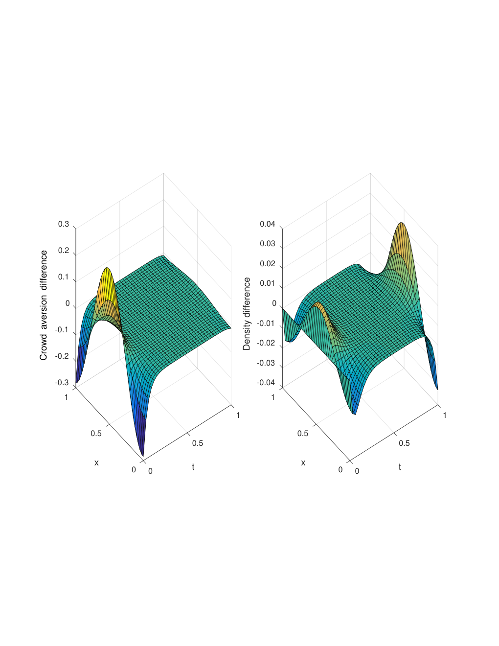
The optimal controls for (5.1) and (5.2) are found by the GDM-scheme of [16]. The convergence of the risk is presented in Figure 2. In Figure 3, a comparison between the solutions of (5.1) and (5.2) is displayed. The crowds behave similarly until time begins to approach t=1t=1. The crowd acting under nonlocal crowd aversion then gathers more densely in the low cost area. Since the crowding experienced by a pedestrian in the nonlocal model is an average over a larger neighborhood, it cares less about pointwise high densities and the benefits of reaching the low cost area around x=0.5x=0.5 has a stronger impact in the nonlocal model, resulting in a more concentrated density. This is visualized in Figure 4, where on the left the difference between crowd aversion penalties,

∫𝕋φr​(x−y)​mnon-local​(t,y)​dy⏟Nonlocal crowd aversion−mlocal​(t,x)⏟Local crowd aversion,\underbrace{\int_{\mathbb{T}}\varphi_{r}(x-y)m_{\text{non-local}}(t,y)dy}_{\text{Nonlocal crowd aversion}}-\underbrace{m_{\text{local}}(t,x)}_{\text{Local crowd aversion}}, (5.6)

is plotted. On the right plot, we display

mnon-local​(t,x)−mlocal​(t,x).m_{\text{non-local}}(t,x)-m_{\text{local}}(t,x). (5.7)

Note that even though the densities differ at t=1t=1, the two crowds experience approximately the same amount of crowding at that time t=1t=1!

Fig 1: The initial density and terminal cost used in the simulations. Initially the pedestrians are crowded around x=0x=0 but they will quickly flatten the density to heed their crowd aversion preferences. The low cost around x=0.5x=0.5 will give the pedestrians an incentive to end up around this part of the domain at t=1t=1.
Fig 2: In each iteration of the GDM the control function aa is updated. The method is run until the risk measure, under local (dashed line) and nonlocal (solid line) crowd aversion, has converged to a minimum.
Fig 3: The optimally controlled density under local (dashed) and non-local (solid) crowd aversion at six instants.
Refer to caption
Fig 4: Differences (Non-local - Local) between the two crowds: crowd aversion penalty (left plot) and density (right plot).

6 Appendix

6.1 Proof of Proposition 4.1

The proof extends the results in [16] to an arbitrary finite number of crowds and to nonlocal crowd aversion.

Proof.

Let the entries in Λ¯\bar{\Lambda} be denoted by λ¯j​k\bar{\lambda}_{jk}. For each j∈[[M]]j\in[\![M]\!],

Jr,Λ¯​(a)−Jr,Λj,det​(aj,a−j)\displaystyle J_{r,\bar{\Lambda}}(a)-J^{j,\text{det}}_{r,\Lambda}(a^{j},a^{-j}) (6.1)
=∑k≠j(∫ℝd∫0T12​|ak​(t,x)|2​mk​(t,x)​dt​dx+∫ℝdΨk​(x)​mk​(T,x)​dx)\displaystyle=\sum_{k\neq j}\left(\int_{\mathbb{R}^{d}}\int_{0}^{T}\frac{1}{2}|a^{k}(t,x)|^{2}m_{k}(t,x)dtdx+\int_{\mathbb{R}^{d}}\Psi_{k}(x)m_{k}(T,x)dx\right)
+∑k,l=1M(∫ℝd∫0TGϕr[mk]Tλ¯k​lmldtdx)−∑k=1M(∫ℝd∫0TGϕr[mk]Tλk​jmjdtdx).\displaystyle+\sum_{k,l=1}^{M}\left(\int_{\mathbb{R}^{d}}\int_{0}^{T}G_{\phi_{r}}[m_{k}]^{T}\bar{\lambda}_{kl}m_{l}dtdx\right)-\sum_{k=1}^{M}\left(\int_{\mathbb{R}^{d}}\int_{0}^{T}G_{\phi_{r}}[m_{k}]^{T}\lambda_{kj}m_{j}dtdx\right).

Note that by symmetry of ϕ\phi, the indices of Gϕ​[mk]G_{\phi}[m_{k}] and mlm_{l} may be swapped under the integral sign and the last line of (6.1) can be rewritten as

∑k,l=1l,k≠jM(∫ℝd∫0TGϕr​[mk]T​λ¯k​l​ml​dt​dx)\displaystyle\sum_{\begin{subarray}{c}k,l=1\\ l,k\neq j\end{subarray}}^{M}\left(\int_{\mathbb{R}^{d}}\int_{0}^{T}G_{\phi_{r}}[m_{k}]^{T}\bar{\lambda}_{kl}m_{l}dtdx\right) (6.2)
+∫ℝd∫0T∑k=1k≠jM(Gϕr[mk]T(λ¯k​j+λj​k−λk​j)mj)+Gϕr[mj]T(λ¯j​j−λj​j)mjdtdx.\displaystyle+\int_{\mathbb{R}^{d}}\int_{0}^{T}\sum_{\begin{subarray}{c}k=1\\ k\neq j\end{subarray}}^{M}\Big(G_{\phi_{r}}[m_{k}]^{T}(\bar{\lambda}_{kj}+\lambda_{jk}-\lambda_{kj})m_{j}\Big)+G_{\phi_{r}}[m_{j}]^{T}(\bar{\lambda}_{jj}-\lambda_{jj})m_{j}dtdx.

The last line vanishes since Λ=Λ¯+Λ¯T−diag​(Λ¯)\Lambda=\bar{\Lambda}+\bar{\Lambda}^{T}-\text{diag}(\bar{\Lambda}) and Jr,Λ¯​(a)−Jr,Λj,det​(aj,a−j)J_{r,\bar{\Lambda}}(a)-J^{j,\text{det}}_{r,\Lambda}(a^{j},a^{-j}) is independent of (aj,mj)(a^{j},m_{j}). Therefore the optimality of a^\hat{a} implies that

Jr,Λj,det​(a^)≤Jr,Λj,det​(aj,a^−j),∀aj∈𝒜d,j∈[[M]].J^{j,\text{det}}_{r,\Lambda}(\hat{a})\leq J^{j,\text{det}}_{r,\Lambda}(a^{j},\hat{a}^{-j}),\quad\forall\ a_{j}\in\mathcal{A}_{d},\ j\in[\![M]\!]. (6.3)

Since (6.3) holds for all j∈[[M]]j\in[\![M]\!], a^\hat{a} is a solution to dMFT-M. ∎

6.2 Proof of Proposition 4.3

This proof is a variation of [15, Proposition 4.2.1] which extends it to an arbitrary finite number of crowds and to nonlocal crowd aversion.

Proof.

Let, for a given ϵ>0\epsilon>0, aϵja_{\epsilon}^{j} be the first order perturbation of a^j\hat{a}^{j} for some arbitrary wjw^{j} such that

aϵj​(t,x):=a^j​(t,x)+ϵ​wj​(t,x)∈𝒜d.a_{\epsilon}^{j}(t,x):=\hat{a}^{j}(t,x)+\epsilon w^{j}(t,x)\in\mathcal{A}_{d}. (6.4)

Let mjϵm_{j}^{\epsilon} satisfy the constraints in (OC) with aϵja^{j}_{\epsilon} and let

mjϵ​(t,x):=m^j​(t,x)+ϵ​hjϵ​(t,x)+𝒪⁡(hjϵ2).m_{j}^{\epsilon}(t,x):=\hat{m}_{j}(t,x)+\epsilon h^{\epsilon}_{j}(t,x)+\mathcal{O}({h^{\epsilon}_{j}}^{2}). (6.5)

Then hjϵh^{\epsilon}_{j} satisfies the equation

{∂hjϵ∂t​(t,x)=12​Tr​[∇2(σ​σT​hjϵ)​(t,x)]−∇⋅(b⁡(t,x,a^j​(t,x))​hjϵ​(t,x))−∇⋅(b⁡(t,x,aϵj​(t,x))−b⁡(t,x,a^j​(t,x)CLOSEϵmϵj(t,x))),hjϵ​(0,x)=0.\left\{\begin{aligned} \frac{\partial h^{\epsilon}_{j}}{\partial t}(t,x)&=\frac{1}{2}\textup{Tr}\left[\nabla^{2}(\sigma\sigma^{T}h^{\epsilon}_{j})(t,x)\right]-\nabla\cdot\left(b(t,x,\hat{a}^{j}(t,x))h^{\epsilon}_{j}(t,x)\right)\\ &-\nabla\cdot\left(\frac{b(t,x,a^{j}_{\epsilon}(t,x))-b(t,x,\hat{a}^{j}(t,x)}{\epsilon}m^{\epsilon}_{j}(t,x))\right),\\ h^{\epsilon}_{j}(0,x)&=0.\end{aligned}\right. (6.6)

Let 𝒥j:ϵ→Jr,Λj,det​(aϵj,a^−j)\mathcal{J}^{j}:\epsilon\rightarrow J^{j,\text{det}}_{r,\Lambda}(a^{j}_{\epsilon},\hat{a}^{-j}). Since the functional is convex, a^\hat{a} solves dMFT-M if and only if

∂𝒥r,Λj∂ϵ​(0)=0,∀wj​ such that ​a^j+ϵ​wj∈𝒜d,∀j∈[[M]].\frac{\partial\mathcal{J}^{j}_{r,\Lambda}}{\partial\epsilon}(0)=0,\quad\forall w^{j}\text{ such that }\hat{a}^{j}+\epsilon w^{j}\in\mathcal{A}_{d},\ \forall\ j\in[\![M]\!]. (6.7)

Condition (6.7) is equivalent to

0=\displaystyle 0= ∫ℝd[∫0T(a^j(t,x)m^j(t,x)⋅wj(t,x)+12|a^j(t,x)|2h0j(t,x)\displaystyle\int_{\mathbb{R}^{d}}\Bigg[\int_{0}^{T}\Bigg(\hat{a}^{j}(t,x)\hat{m}_{j}(t,x)\cdot w^{j}(t,x)+\frac{1}{2}|\hat{a}^{j}(t,x)|^{2}h^{0}_{j}(t,x) (6.8)
+2​λj​j​(∫ℝdϕr​(x−y)​m^j​(t,y)​dy)​hj0​(t,x)\displaystyle+2\lambda_{jj}\left(\int_{\mathbb{R}^{d}}\phi_{r}(x-y)\hat{m}_{j}(t,y)dy\right)h^{0}_{j}(t,x)
+∑k≠jMλj​k(∫ℝdϕr(x−y)m^k(t,y)dy)h0k(t,x))dt+Ψj(x)h0j(T,x)]dx\displaystyle+\sum_{k\neq j}^{M}\lambda_{jk}\left(\int_{\mathbb{R}^{d}}\phi_{r}(x-y)\hat{m}_{k}(t,y)dy\right)h^{0}_{k}(t,x)\Bigg)dt+\Psi_{j}(x)h^{0}_{j}(T,x)\Bigg]dx

where hj0h^{0}_{j} is the solution of (6.6) in the limit ϵ→0\epsilon\rightarrow 0. Recall that Λ′=12​(Λ+diag​(Λ))\Lambda^{\prime}=\frac{1}{2}(\Lambda+\text{diag}(\Lambda)). Since pp satisfies the adjoint equation, Ψj​(x)=pj​(T,x)\Psi_{j}(x)=p_{j}(T,x) and

∫ℝdpj​(T,x)​hj0​(T,x)​𝑑x\displaystyle\int_{\mathbb{R}^{d}}p_{j}(T,x)h^{0}_{j}(T,x)dx (6.9)
=∫ℝd∫0T{−12|aj(t,x)|2−2λj​j(∫ℝdϕr(x−y)m^j(t,y)dy)\displaystyle=\int_{\mathbb{R}^{d}}\int_{0}^{T}\Bigg\{-\frac{1}{2}|a^{j}(t,x)|^{2}-2\lambda_{jj}\left(\int_{\mathbb{R}^{d}}\phi_{r}(x-y)\hat{m}_{j}(t,y)dy\right)
−∑k≠jMλj​k(∫ℝdϕr(x−y)m^k(t,y)dy)−b(t,x,a^j(t,x))⋅∇pj(t,x)\displaystyle-\sum_{k\neq j}^{M}\lambda_{jk}\left(\int_{\mathbb{R}^{d}}\phi_{r}(x-y)\hat{m}_{k}(t,y)dy\right)-b(t,x,\hat{a}^{j}(t,x))\cdot\nabla p_{j}(t,x)
−12Tr[σσT∇2pj(t,x)]}h0j(t,x)\displaystyle-\frac{1}{2}\textup{Tr}\left[\sigma\sigma^{T}\nabla^{2}p_{j}(t,x)\right]\Bigg\}h^{0}_{j}(t,x)
+{12Tr[∇2(σσTh0j)(t,x)]−∇⋅(b(t,x,a^j(t,x))h0j(t,x))\displaystyle+\Bigg\{\frac{1}{2}\textup{Tr}\left[\nabla^{2}(\sigma\sigma^{T}h^{0}_{j})(t,x)\right]-\nabla\cdot\left(b(t,x,\hat{a}^{j}(t,x))h^{0}_{j}(t,x)\right)
−∇⋅(Dajb(t,x,a^j(t,x))wj(t,x)m^j(t,x))}pj(t,x)dtdx.\displaystyle-\nabla\cdot\left(D_{a^{j}}b(t,x,\hat{a}^{j}(t,x))w^{j}(t,x)\hat{m}_{j}(t,x)\right)\Bigg\}p_{j}(t,x)dtdx.

Inserting (6.9) into (6.8) yields

∫ℝd∫0T(a^j(t,x)+Dajb(t,x,a^j(t,x))T∇pj(t,x))⋅wj(t,x)mj^(t,x)dxdt=0.\int_{\mathbb{R}^{d}}\int_{0}^{T}\left(\hat{a}^{j}(t,x)+D_{a^{j}}b(t,x,\hat{a}^{j}(t,x))^{T}\nabla p_{j}(t,x)\right)\cdot w_{j}(t,x)\hat{m_{j}}(t,x)dxdt=0. (6.10)

Note that this since (6.10) holds for all j∈[[M]]j\in[\![M]\!], a^\hat{a} satisfies the optimality condition in Theorem 4.2 and therefore a^\hat{a} is a solution to (OC) by Theorem 4.2. ∎

References

  • [2] Achdou, Y., Bardi, M. and Cirant, M. [2017], ‘Mean field games models of segregation’, Mathematical Models and Methods in Applied Sciences 27(01), 75–113.
  • [3] Achdou, Y. and Laurière, M. [2015], ‘On the system of partial differential equations arising in mean field type control’, arXiv preprint arXiv:1503.05044 .
  • [4] Achdou, Y. and Laurière, M. [2016a], ‘Mean field type control with congestion’, Applied Mathematics & Optimization 73(3), 393–418.
  • [5] Achdou, Y. and Laurière, M. [2016b], ‘Mean field type control with congestion (ii): An augmented lagrangian method’, Applied Mathematics & Optimization 74(3), 535–578.
  • [6] Andersson, D. and Djehiche, B. [2011], ‘A maximum principle for sdes of mean-field type’, Applied Mathematics & Optimization 63(3), 341–356.
  • [7] Bardi, M. and Cirant, M. [2017], ‘Uniqueness of solutions in mean field games with several populations and Neumann conditions’, arXiv preprint arXiv:1709.02158 .
  • [8] Bensoussan, A., Frehse, J., Yam, P. et al. [2013], Mean field games and mean field type control theory, Vol. 101, Springer.
  • [9] Cirant, M. [2015], ‘Multi-population mean field games systems with Neumann boundary conditions’, Journal de Mathématiques Pures et Appliquées 103(5), 1294–1315.
  • [10] Feleqi, E. [2013], ‘The derivation of ergodic mean field game equations for several populations of players’, Dynamic Games and Applications 3(4), 523–536.
  • [11] Huang, M., Malhamé, R. P., Caines, P. E. et al. [2006], ‘Large population stochastic dynamic games: closed-loop mckean-vlasov systems and the nash certainty equivalence principle’, Communications in Information & Systems 6(3), 221–252.
  • [12] Kallenberg, O. [2006], Foundations of modern probability, Springer Science & Business Media.
  • [13] Karatzas, I. and Shreve, S. [2012], Brownian motion and stochastic calculus, Vol. 113, Springer Science & Business Media.
  • [14] Kolokoltsov, V. and Troeva, M. [2015], ‘On the mean field games with common noise and the mckean-vlasov spdes’, arXiv preprint arXiv:1506.04594 .
  • [15] Lachapelle, A. [2010], Quelques problèmes de transport et de contrôle en économie: aspects théoriques et numériques, PhD thesis, Université Paris Dauphine-Paris IX.
  • [16] Lachapelle, A. and Wolfram, M.-T. [2011], ‘On a mean field game approach modeling congestion and aversion in pedestrian crowds’, Transportation research part B: methodological 45(10), 1572–1589.
  • [17] Lasry, J.-M. and Lions, P.-L. [2007], ‘Mean field games’, Japanese Journal of Mathematics 2(1), 229–260.
  • [18] Lions, P.-L. [n.d.], ‘Cours du Collège de France’. Accessed: 2017-09-29.
    https://www.college-de-france.fr/site/en-pierre-louis-lions/course-2011-2012.htm
  • [19] Naldi, G., Pareschi, L. and Toscani, G. [2010], Mathematical modeling of collective behavior in socio-economic and life sciences, Springer Science & Business Media.
  • [20] Oelschläger, K. [1985], ‘A law of large numbers for moderately interacting diffusion processes’, Zeitschrift für Wahrscheinlichkeitstheorie und verwandte Gebiete 69(2), 279–322.
  • [21] Parthasarathy, K. R. [1967], Probability measures on metric spaces, Vol. 352, American Mathematical Soc.
  • [22] Sznitman, A.-S. [1991], Topics in propagation of chaos, in ‘Ecole d’été de probabilités de Saint-Flour XIX—1989’, Springer, pp. 165–251.
  • [23] Tcheukam, A., Djehiche, B. and Tembine, H. [2016], Evacuation of multi-level building: Design, control and strategic flow, in ‘Control Conference (CCC), 2016 35th Chinese’, IEEE, pp. 9218–9223.
  • [24] Yamada, T., Watanabe, S. et al. [1971], ‘On the uniqueness of solutions of stochastic differential equations’, Journal of Mathematics of Kyoto University 11(1), 155–167.
  • [25] Yong, J. and Zhou, X. Y. [1999], Stochastic controls: Hamiltonian systems and HJB equations, Vol. 43, Springer Science & Business Media.