On the Geometry of Bayesian Inference
Abstract
We provide a geometric interpretation to Bayesian inference that allows us to introduce a natural measure of the level of agreement between priors, likelihoods, and posteriors. The starting point for the construction of our geometry is the simple observation that the marginal likelihood can be regarded as an inner product between the prior and the likelihood. A key concept in our geometry is that of compatibility, a measure which is based on the same construction principles as Pearson correlation, but which can be used to assess how much the prior agrees with the likelihood, to gauge the sensitivity of the posterior to the prior, and to quantify the coherency of the opinions of two experts. Estimators for all the quantities involved in our geometric setup are discussed, which can be directly computed from the posterior simulation output. Some examples are used to illustrate our methods, including data related to on-the-job drug usage, midge wing length, and prostate cancer.
keywords: Bayesian inference; Geometry; Harmonic mean estimator; Hilbert spaces; Marginal likelihood.
1 Introduction
Assessing the influence that prior distributions and/or likelihoods have on posterior inference has been a topic of research for some time. One commonly used ad-hoc method suggests fitting a Bayes model using a few competing priors, then visually (or numerically) assessing changes in the posterior as a whole or using some pre-specified posterior summary. More rigorous approaches have also been developed. Lavine (1991) developed a framework to assess sensitivity of posterior inference to sampling distribution (likelihood) and the priors. Berger (1991) introduced the concept of Bayesian robustness which includes perturbation models (see also Berger and Berliner 1986). More recently, Evans and Jang (2011) have compared information available in two competing priors. Related to this work, Gelman et al. (2008) advocates the use of so-called weakly informative priors that purposely incorporate less information than available as a means of regularizing. Work has also been dedicated to the so-called prior–data conflict (Evans and Moshonov, 2006; Walter and Augustin, 2009; Al Labadi and Evans, 2016). Such conflict can be of interest in a wealth of situations, such as for evaluating how much prior and likelihood information are at odds at the node level in a hierarchical model (see Scheel, Green and Rougier, 2011, and references therein). Regarding sensitivity of the posterior distribution to prior specifications, Lopes and Tobias (2011) provide a fairly accessible overview.
We argue that a geometric representation of the prior, likelihood, and posterior distribution encourages understanding of their interplay. Considering Bayes methodologies from a geometric perspective is not new, but none of the existing geometric perspectives has been designed with the goal of providing a summary on the agreement or impact that each component of Bayes theorem has on inference and predictions. Aitchison (1971) used a geometric perspective to build intuition behind each component of Bayes theorem, Shortle and Mendel (1996) used a geometric approach to draw conditional distributions in arbitrary coordinate systems, and Agarawal and Daumé (2010) argued that conjugate priors of posterior distributions belong to the same geometry giving an appealing interpretation of hyperparameters. Zhu, Ibrahim and Tang (2011) defined a manifold on which a Bayesian perturbation analysis can be carried out by perturbing data, prior and likelihood simultaneously, and Kurtek and Bharath (2015) provide an elegant geometric construction which allows for Bayesian sensitivity analysis based on the so-called -compatibility class and on comparison of posterior inferences using the Fisher–Rao metric.
In this paper, we develop a geometric setup along with a set of metrics that can be used to provide an informative preliminary ‘snap-shot’ regarding comparisons between prior and likelihood (to assess the level of agreement between prior and data), prior and posterior (to determine the influence that prior has on inference), and prior versus prior (to compare ‘informativeness’—i.e., a density’s peakedness—and/or congruence of two competing priors). To this end, we treat each component of Bayes theorem as an element of a geometry formally constructed using concepts from Hilbert spaces and tools from abstract geometry. Because of this, it is possible to calculate norms, inner products, and angles between vectors. Not only do each of these numeric summaries have intuitively appealing individual interpretations, but they may also be combined to construct a unitless measure of compatibility, which can be used to assess how much the prior agrees with the likelihood, to gauge the sensitivity of the posterior to the prior, and to quantify the coherency of the opinions of two experts. Estimating our measures of level of agreement is straightforward and can actually be carried out within an MCMC algorithm. An important advantage of our setting is that it offers a direct link to Bayes theorem, and a unified treatment that can be used to assess the level of agreement between priors, likelihoods, and posteriors—or functionals of these. To streamline the illustration of ideas, concepts, and methods we reference the following example (Christensen et al., 2011, pp. 26–27) throughout the article.
On-the-job drug usage toy example
Suppose interest lies in estimating the proportion of US transportation industry workers that use drugs on the job. Suppose workers were selected and tested with the 2nd and 7th testing positive. Let with denoting that the th worker tested positive and otherwise. Let , for , and , for . Then, with and , where .
Some natural questions our treatment of Bayes theorem will answer are: How compatible is the likelihood with this prior choice? How similar are the posterior and prior distributions? How does the choice of compare to other possible prior distributions? While the drug usage example provides a recurring backdrop that we consistently call upon, additional examples are used throughout the paper to illustrate our methods.
In Section 2 we introduce the geometric framework in which we work and provide definitions and interpretations along with examples. Section 3 considers extensions of the proposed setup, Section 4 contains computational details, and Section 5 provides a regression example illustrating utility of our metric. Section 6 conveys some concluding remarks. Proofs are given in the supplementary materials.
2 Bayes geometry
2.1 A geometric view of Bayes theorem
Suppose the inference of interest is over a parameter which takes values on . We consider the space of square integrable functions , and use the geometry of the Hilbert space , with inner-product
| (1) |
The fact that is a Hilbert space is often known in mathematical parlance as the Riesz–Fischer theorem; for a proof see Cheney (2001, p. 411). Borrowing geometric terminology from linear spaces, we refer to the elements of as vectors, and assess their ‘magnitudes’ through the use of the norm induced by the inner product in (1), i.e., .
The starting point for constructing our geometry is the observation that Bayes theorem can be written using the inner-product in (1) as follows
| (2) |
where denotes the likelihood, is a prior density, is the posterior density and is the marginal likelihood or integrated likelihood. The inner product in (1) naturally leads to considering and that are in , which is compatible with a wealth of parametric models and proper priors. By considering , , and as vectors with different magnitudes and directions, Bayes theorem simply indicates how one might recast the prior vector so as to obtain the posterior vector. The likelihood vector is used to enlarge/reduce the magnitude and suitably tilt the direction of the prior vector in a sense that will be made precise below.
The marginal likelihood is simply the inner product between the likelihood and the prior, and hence can be understood as a measure of agreement between the prior and the likelihood. To make this more concrete, define the angle measure between the prior and the likelihood as
| (3) |
Since and are nonnegative, the angle between the prior and the likelihood can only be acute or right, i.e., . The closer is to , the greater the agreement between the prior and the likelihood. Conversely, the closer is to , the greater the disagreement between prior and likelihood. In the pathological case where (which requires the prior and the likelihood to have all of their mass on disjoint sets), we say that the prior is orthogonal to the likelihood. Bayes theorem is incompatible with a prior being orthogonal to the likelihood as indicates that , thus leading to a division by zero in (2). Similar to the correlation coefficient for random variables in —with denoting the Borel sigma-algebra over the sample space —, our target object of interest is given by a standardized inner product
| (4) |
The quantity quantifies how much an expert’s opinion agrees with the data, thus providing a natural measure of the level of agreement between prior and data.
Before exploring (4) more fully by providing interpretations and properties we concretely define how the term ‘geometry’ will be used throughout the paper. The following definition of abstract geometry can be found in Millman and Parker (1991, p. 17).
Definition 1 (Abstract geometry).
An abstract geometry consists of a pair , where the elements of set are designed as points, and the elements of the collection are designed as lines, such that:
- 1.
For every two points , there is a line .
- 2.
Every line has at least two points.
Our abstract geometry of interest is , where and the set of all lines is
| (5) |
Hence, in our setting points can be, for example, prior densities, posterior densities, or likelihoods, as long as they are in . Lines are elements of , as defined in (5), so that for example if and are densities, line segments in our geometry consist of all possible mixture distributions which can be obtained from and , i.e.,
| (6) |
A related interpretation of two-component mixtures as straight lines can be found in Marriott (2002, p. 82).
Vectors in are defined through the difference of elements in . For example, let and let . Then , and hence can be regarded both as a point and as a vector. If are vectors then we say that and are collinear if there exists , such that . Put differently, we say and are collinear if , for all .
For any two points in the geometry under consideration, we define their compatibility as a standardized inner product (with (4) being a particular case).
Definition 2 (Compatibility).
The compatibility between points in the geometry under consideration is defined as
| (7) |
The concept of compatibility in Definition 2 is based on the same construction principles as the Pearson correlation coefficient, which would be based however on the inner product
| (8) |
instead of the inner product in (1). However, compatibility is defined for priors, posteriors, and likelihoods in equipped with the inner product (1), whereas Pearson correlation works with random variables in equipped with the inner product (8). Our concept of compatibility can be used to evaluate how much the prior agrees with the likelihood, to measure the sensitivity of the posterior to the prior, and to quantify the level of agreement of elicited priors. As an illustration consider the following example.
Example 1.
Consider the following densities , , , and . Note that , , and; further, , thus implying that . Also, and hence .
As can be observed in Example 1, is a natural measure of distinctiveness of two densities. In addition, Example 1 shows us how different distributions can be associated to the same norm and angle. Hence, as expected, any Cartesian representation , will only allow us to represent some features of the corresponding distributions, but will not allow us to identify the distributions themselves.
(i)
(ii)
To build intuition regarding , we provide Figure 1, where is set to while varies according to and . Figure 1 (i) corresponds to fixing and varying while in the right plot is fixed and varies. Notice that in plot (i) corresponds to distributions whose means are approximately 3 standard deviations apart while a corresponds to distributions whose means are approximately 0.65 standard deviations apart. Connecting specific values of to specific standard deviation distances between means seems like a natural way to quickly get a rough idea of relative differences between two distributions. In Figure 1 (ii) it appears that if both distributions are centered at the same value, then one distribution must be very disperse relative to the other to produce values that are small (e.g., ). This makes sense as there always exists some mass intersection between the two distributions considered. Thus, —to which we refer as compatibility—can be regarded as a measure of the level of agreement between prior and data. Some further comments regarding our geometry are in order:
- •
Two different densities and cannot be collinear: If , then , otherwise .
- •
A density can be collinear to a likelihood: If the prior is Uniform then , and hence the posterior is collinear to the likelihood, i.e., in such a case the posterior simply consists of a renormalization of the likelihood.
- •
Two likelihoods can be collinear: Let and be the likelihoods based on observing and , respectively. The strong likelihood principle states that if , then the same inference should be drawn from both samples (Berger and Wolpert, 1988). According to our geometry, this would mean that likelihoods with the same direction yield the same inference.
As a final comment on reparametrizations of the model, interpretations of compatibility should keep a fixed parametrization in mind. That is, we do not recommend comparing prior–likelihood compatibility for models with different parametrizations. Further comments on reparametrizations will be given below in Sections 2.3, 2.4, and 3.2.
2.2 Norms and their interpretation
As is comprised of function norms, we dedicate some exposition to how one might interpret these quantities. We start by noting that in some cases the norm of a density is linked to the variance, as can be seen in the following example.
Example 2.
Let and let denote its corresponding density. Then, it holds that , where the variance of is . Next, consider a Normal model with known variance and let denote its corresponding density. It can be shown that which is a function of .
The following proposition explores how the norm of a general prior density, , relates with that of a Uniform density, .
Proposition 1.
Let with where denotes the Lebesgue measure. Consider : a probability density with and let denote a Uniform density on , then
| (9) |
Since is constant, increases as ’s mass becomes more concentrated (or less Uniform). Thus, as can be seen from (9), is a measure of how much differs from a Uniform distribution over . This interpretation cannot be applied to ’s that do not have finite Lebesgue measure as there is no corresponding proper Uniform distribution. Nonetheless, the notion that the norm of a density is a measure of its peakedness may be applied whether or not has finite Lebesgue measure. To see this, evaluate on a grid and consider the vector , with for . The larger the norm of the vector , the higher the indication that certain components would be far from the origin—that is, would be peaking for certain in the grid. Now, think of a density as a vector with infinitely many components (its value at each point of the support) and replace summation by integration to get the norm. Therefore, can be used to compare the ‘informativeness’ of two competing priors with indicating that is less informative.
Further reinforcing the idea that the norm is related to the peakedness of a distribution, there is an interesting connection between and the (differential) entropy (denoted by ) which is described in the following proposition.
Proposition 2.
Suppose is a continuous density on a compact , and that is differentiable on . Let . Then, it holds that
| (10) |
for some .
The expansion in (10) hints that the norm of a density and the entropy should be negatively related, and hence as the norm of a density increases, its mass becomes more concentrated. In terms of priors, this suggests that priors with a large norm should be more ‘peaked’ relative to priors with a smaller norm. Therefore, the magnitude of a prior appears to be linked to its peakedness (as is demonstrated in (9) and in Example 2). While this might also be viewed as ‘informativeness,’ the density has a higher norm if than if , possibly placing this interpretation at odds with the notion that and represent ‘prior successes’ and ‘prior failures’ in the Beta–Binomial setting. As will be further discussed in Section 2.5, a reviewer recognized that this seeming paradox is a consequence of the parameterization employed and is avoided when using the log-odds as the parameter.
As can be seen from (10), the connection between entropy and is an approximation at best. Just as a first-order Taylor expansion provides a poor polynomial approximation for points that are far from the point under which the expansion is made, the expansion in (10) will provide a poor entropy approximation when is not similar to a standard Uniform-like distribution . However, since , the approximation is exact for a standard Uniform-like distribution. We end this discussion by noting that integrals related to also appear in physical models on -spaces and they are usually interpreted as the total energy of a physical system (Hunter and Nachtergaele, 2005, p. 142), and there is considerable frequentist literature on the estimation of the integrated square of a density (see Giné and Nickl, 2008, and references therein). Now, to illustrate the information that and provide, we consider the example described in Section 1.
(i)
(ii)
Example 3 (On-the-job drug usage toy example, cont. 1).
From the example in the Introduction we have with and . The norm of the prior, posterior, and likelihood are respectively given by
| (11) |
and , with , and
where .
Figure 2 (i) plots and Figure 2 (ii) plots as functions of and . We highlight the prior values which were employed by Christensen et al. (2011). Because prior densities with large norms will be more peaked relative to priors with small norms, is more peaked than (Uniform prior) indicating that is more ‘informative’ than . The norm of the posterior for these same pairs is and , meaning that the posteriors will have mass more concentrated than the corresponding priors. The lines found in Figure 2 (ii) represent boundary lines such that all pairs that fall outside of the boundary produce which indicates that the prior is more peaked than the posterior (typically an undesirable result). If we used an extremely peaked prior, say , then we would get and indicating that the peakedness of the prior and posterior densities is essentially the same.
Considering , it follows that
| (12) |
with and . Figure 3 (i) plots values of as a function of prior parameters and with being highlighted indicating a great deal of agreement with the likelihood. In this example a lack of prior–data compatibility would occur (e.g., ) for priors that are very peaked at or for priors that place substantial mass at .
(i)
(ii)
(iii)
2.3 Angles between other vectors
As mentioned, we are not restricted to use only to compare and . Angles between densities, and between likelihoods and densities or even between two likelihoods are available. We explore these options further using the example provided in the Introduction.
Example 4 (On-the-job drug usage toy example, cont. 2).
Extending Example 3 and (12) we calculate
with and ; for and ,
To visualize how the hyperparameters influence and we provide Figures 3 (ii) and (iii). Figure 3 (ii) again highlights the prior used in Christensen et al. (2011) with ; see solid dot (). This value of implies that both prior and posterior are concentrated on essentially the same subset of , indicating a large amount of agreement between them. Disagreement between prior and posterior takes place with priors concentrated on high probabilities of being greater than 0.8. In Figure 3 (iii), is largest when is close to (the distribution of ) and gradually drops off as becomes more peaked and/or less symmetric.
In the next example, we use another data illustration to demonstrate the application of to a two-parameter model.
Example 5 (Midge wing length data).
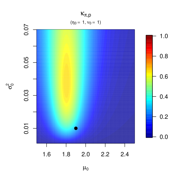
Let , and and ; we refer to this conjugate prior distribution as . In comparing and , may be expressed as,
| (13) |
with

(i)
(ii)
Note that (13) (whose derivation can be found in Section 5.1 of the Supplementary Materials) may also be used to compute , since , with
Computation of also adheres to Equation (13) if and because then is collinear to . Hoff (2009, pp. 72–76) applied this model to a dataset of nine midge wing lengths, where he set , , , and , while and . This yields , and thus the agreement between the prior and posterior is not particularly strong. Figure 4 (i) displays , as a function of and while fixing and . To evaluate how is affected by and , the analogous plot is displayed as Figure 4 (ii) when these values are fixed at and ; these alternative values for and are those which allow the compatibility between the prior and likelihood to be maximised. It is apparent from Figure 4 that a larger increases substantially, and a simultaneous increase of and would further propel this increase.
Some comments on reparametrizations are in order. We focus on the case of compatibility between two priors with a single parameter, but the rationale below also applies to compatibility between a prior and posterior, and in multiparameter settings. Let and ; further, let be a monotone increasing function, with range , and let
be prior densities of the transformed parameters, and . It thus follows that
The version of compatibility discussed in this section is thus invariant to linear transformations of the parameter. A variant to be discussed in Section 3.2 is more generally invariant to monotone increasing transformations.
2.4 Max-compatible priors and maximum likelihood estimators
In Example 3, we briefly alluded to a connection between priors maximising prior–likelihood compatibility (to be termed as max-compatible priors) and maximum likelihood (ML) estimators, on which we now elaborate. Below, we use the notation to denote a prior on , with are hyperparameters, and where and . (Think of the Beta–Binomial model, where , and .)
Definition 3 (Max-compatible prior).
Let , and let be a family of priors for . If there exists , such that , the prior is said to be max-compatible, and is said to be a max-compatible hyperparameter.
The max-compatible hyperparameter, , is by definition a random vector, and thus a max-compatible prior density is a random function. Geometrically, a prior is max-compatible if and only if it is collinear to the likelihood in the sense that if and only if , for all .
The following example suggests there could be a connection between the ML estimator of and the max-compatibility parameter .
Example 6 (Beta–Binomial).
Let , and suppose . Here, with It can be shown that the max-compatible prior is , where , and , so that
| (14) |
with .
A natural question is whether there always exists a function , as in (14), linking the max-compatible parameter with the ML estimator? The following theorem addresses this.
Proposition 3.
Let , and let be the ML estimator of . In addition, let be a family of priors for . If there exists a unimodal max-compatible prior, then
Proposition 3 states that the mode of the max-compatible prior coincides with the ML estimator, and in Example 6, is indeed the mode of a Beta prior. A comment on parametrizations is in order. A corollary to Proposition 3 is that, due to invariance of ML estimators, if is the mode of the max-compatible prior for and is a function, then is the mode of the max-compatible prior of the transformed parameter . Formally,
with and where is the range of .
The max-compatible prior is a ‘prior’ to the extent that it belongs to a family of priors, but it is basically a posterior distribution (it depends on the data). Also, there are some links between the max-compatible prior and Hartigan’s maximum likelihood prior (Hartigan, 1998), which will be clarified in Section 2.5.
2.5 Compatibility in the exponential family
We now consider compatibility in the exponential family with density
for given functions and , and with denoting the so-called cumulant function. Given a random sample from an exponential family, , it follows that
The conjugate prior is known to be
| (15) |
where and are parameters, and
| (16) |
The posterior density is , with defined as in (15); cf Diaconis and Ylvisaker (1979). In this context, compatibility can be expressed using normalizing constants from various members of the conjugate prior family as follows
| (17) |
for for which the normalizing constants in (17) are defined. The max-compatible prior in the exponential family is given by the following data-dependent prior
| (18) |
with as in (15). Special cases of the results in (17) and (18) were manifest for instance in (12), Example 4, and Example 6.
As pointed out by a reviewer, working with the canonical parametrization brings numerous advantages, especially when measuring compatibility. Since the parametrization of a model is arbitrary (and hence the interpretation of the parameter may be different for each model) it is desirable to work in terms of a parametrization that preserves the same meaning regardless of the model under consideration. For exponential families, a natural choice is the canonical parameter . For one thing, the conjugate prior on the canonical parameter always exists under very general conditions (Diaconis and Ylvisaker, 1979). In contrast, the conjugate family for an alternative parametrization as defined in (15) can be empty; see Gutiérrez-Peña and Smith (1995, Example 1.2). In what follows, we revisit the Beta–Binomial setting and showcase yet another advantage of working with the canonical parametrization.
Example 7.
Let be the natural parameter of and consider the prior for as . The conjugate prior for the natural parameter is
It is readily apparent that
More informative priors (i.e. larger values of and/or ) will always be more ‘peaked’ than less informative ones, and there is no need to constrain the range of values of the hyperparameters to the set , as it was the case in (11). Finally, note that the max-compatible prior under the canonical parametrization is , whereas the max-compatible prior under the parametrization used earlier in Example 6 was .
There are some links between the max-compatible prior introduced in Section 2.4 and Hartigan’s maximum likelihood prior (Hartigan, 1998). In the context of the exponential family, Hartigan’s maximum likelihood prior is a uniform distribution on the canonical parameter . Equation (18) then implies that the max-compatible prior on the canonical parameter , can be regarded as a posterior derived from Hartigan’s maximum likelihood prior.
3 Extensions
3.1 Local prior–likelihood compatibility
In some cases, when assessing the level of agreement between prior and likelihood, integrating over may not be feasible, but one can still assess the level of agreement over priors supported on a subset of the parameter space. Below represents the parameter space and denotes the support of the prior. More specifically, let be a prior supported on . We define local prior–likelihood compatibility as
| (19) |
where , , and . Note that
and thus if , then . In practice, we recommend using standard likelihood–prior compatibility (4) instead of its local version (19), with the exception of situations for which the likelihood is square integrable over but not over . To illustrate that (19) could be well defined even if (4) is not, suppose with and , for . In this pathological single-observation case (4) would not be defined, while it follows that,
Since (4) only assesses the level of agreement locally—that is, over —the values of (4) and (19) are not directly comparable. A local can be analogously defined to (19).
3.2 Affine-compatibility
We now comment on a version of our geometric setup where one no longer focuses directly on angles between priors, likelihoods, and posteriors, but on functions of these. Specifically, we consider the following measures of agreement,
| (20) |
Some affine-compatibilities in (20) are Hellinger affinities (van der Vaart, 1998, p. 211), and thus have links with Kurtek and Bharath (2015) and Roos et al. (2015). Action does not always takes place at the Hilbert sphere, given the need of considering . Local versions of prior–likelihood and likelihood–posterior affine-compatibility, and , can be readily defined using the same principles as in Section 3.1.
It is a routine exercise to prove that max-compatible hyperparameters also maximise , and thus all comments on Section 2.4 also apply to prior–likelihood affine-compatibility. In terms of affine-compatibility in the exponential family, following the same notation as in Section 2.5, it can be shown that
| (21) |
with as defined in (16).
Affine-compatibility between priors and posteriors is invariant to monotone increasing parameter transformations, as a consequence of properties of the Hellinger distance (Roos and Held, 2011, p. 267). Affine-compatibility counterparts of all data examples are available from the supplementary materials; the conclusions are tantamount to the ones using compatibility.
4 Posterior and prior mean-based estimators of compatibility
In many situations closed form estimators of and are not available. This leads to considering algorithmic techniques to obtain estimates. As most Bayes methods resort to MCMC methods it would be appealing to express and as functions of posterior expectations and employ MCMC iterates to estimate them. For example, can be expressed as
| (22) |
where is the expected value with respect to the posterior density. A natural Monte Carlo estimator would then be
| (23) |
where denotes the th MCMC iterate of . Consistency of such an estimator follows trivially by the ergodic theorem and the continuous mapping theorem, but there is an important issue regarding its stability. Unfortunately, (22) includes an expectation that contains in the denominator and therefore (23) inherits the undesirable properties of the so-called harmonic mean estimator (Newton and Raftery, 1994). It has been shown that even for simple models this estimator may have infinite variance (Raftery et al. 2007), and has been harshly criticized for, among other things, converging extremely slowly. Indeed, as argued by Wolpert and Schmidler (2012, p. 655): “the reduction of Monte Carlo sampling error by a factor of two requires increasing the Monte Carlo sample size by a factor of , or in excess of when , rendering [the harmonic mean estimator] entirely untenable.”
An alternate strategy is to avoid writing as a function of harmonic mean estimators and instead express it as a function of posterior and prior expectations. For example, consider
| (24) |
where . Now the Monte Carlo estimator is
| (25) |
where denotes the th draw of from , which can also be sampled within the MCMC algorithm. Although representations (24) and (25) could in principle suffer from numerical instability for diffuse priors, they behave much better in practice than (22) and (23). To see this, Figure 5 contains running estimates of using (23) and (25) for Example 3 with three prior parameter specifications, namely: , , and ; the true for each prior specification is also provided. It is fairly clear that displays slow convergence and large variance, while converges quickly.
The next proposition contains prior and posterior mean-based representations of geometric quantities that can be readily used for constructing Monte Carlo estimators.
Proposition 4.
Let be a prior supported on , with and be defined as in (19), and let and . Then,
Similar derivations can be used to obtain posterior and prior mean-based estimators for affine-compatibility; see supplementary materials. In the next section we provide an example that requires the use of Proposition 4 to estimate and .
5 Example: Regression shrinkage priors
5.1 Compatibility of Gaussian and Laplace priors
The linear regression model is ubiquitous in applied statistics. In vector form, the model is commonly written as
| (26) |
where , is a design matrix, is a -vector of regression coefficients, and is an unknown idiosyncratic variance parameter; the experiments below employ . We consider Gaussian and Laplace prior distributions for . As documented in Park and Casella (2008) and Kyung et al. (2010) ridge regression and produce the same regularization on while the lasso produces the same regularization on as assuming (where ). Below, we use to denote a Gaussian prior and a Laplace. Further, we set which ensures that for all .
5.2 Prostate cancer data example
We now consider the prostate cancer data example found in Hastie, Tibshirani and Friedman (2008, Section 3.4) to explore the ‘informativeness’ of and various compatibility measures for and . In this example the response variable is the level of prostate-specific antigens measured on 97 males. Eight other clinical measurements (such as age and log prostate weight) were also measured and are used as covariates.
We first evaluate the ‘informativeness’ of the two priors by computing and and then their compatibility using . All calculations employed Proposition 4 and results for a sequence of values are provided in Figure 6. Focusing on the left plot of Figure 6 it appears that for small values of the , , indicating that the Laplace prior is more peaked than the Gaussian. Thus, even though the Laplace has thicker tails, it is more ‘informative’ relative to the Gaussian. This corroborates the lasso penalization’s ability to shrink coefficients to zero (something ridge regulation lacks). As increases the two norms converge as both spread their mass more uniformly. The right plot of Figure 6 depicts as a function of . When is centered at zero, then is constant over values of which means that mass intersection when both priors are centered at zero is not influenced by tail thickness. Compare this to values when is not centered at zero [i.e., or ]. For the former, increases as intersection of prior and posterior mass increases. For the latter, must be greater than two for there to be any substantial mass intersection as remains essentially at zero.
We now fit model (26) to the cancer data and use Proposition 4 to calculate various measures of compatibility. Without loss of generality we centered the so that does not include an intercept and standardized each of the eight covariates to have mean zero and standard deviation one. The results are available from Figure 7.
Focusing on the left plot of Figure 7 the small values of and indicate the existence of prior–data incompatibility. For small values of , indicating more compatibility between prior and data for the Gaussian prior. Prior–posterior compatibility () is very similar for both priors with that for being slightly smaller when is close to . The slightly higher value for the Gaussian prior implies that it has slightly more influence on the posterior than the Laplace. Similarly, the Laplace prior seems to produce larger values than that of the Gaussian prior and approaches one quicker than indicating a larger amount of posterior-data compatibility. Overall, it appears that the Gaussian prior has more influence on the resulting posterior distribution relative to the Laplace when updating knowledge via Bayes theorem. Similar conclusions as above would be reached by considering affine-compatibility; see supplementary materials.
6 Discussion
Bayesian inference is regarded from the viewpoint of the geometry of Hilbert spaces. The framework offers a direct connection to Bayes theorem, and a unified treatment that can be used to quantify the level of agreement between priors, likelihoods, and posteriors—or functions of these. The possibility of developing new probabilistic models, obeying the geometrical principles discussed here, offering alternative ways to recast the prior vector using the likelihood vector remains to be explored. In terms of high-dimensional extensions, one could anticipate that as the dimensionality increases, there is increased potential for disagreement between two distributions. Consequently, would generally diminish as additional parameters are added, ceteris paribus, but a suitable offsetting transformation of could result in a measure of ‘per parameter’ agreement.
Some final comments on related constructions are in order. Compatibility as set in Definition 2 includes as a particular case the measures of niche overlap in Slobodchikoff and Schulz (1980). Peakedness as discussed in here should not be confused with the concept of Birnbaum (1948). The geometry in Definition 1 has links with the so-called affine space and thus the geometrical framework discussed above is different but has many similarities with that of Marriott (2002) and also with the mixture geometry of Amari (2016). A key difference is that the latter approaches define an inner product with respect to a density which is the basis of the construction of the Fisher information while here we define it simply as the product of two functions in , and connect the construction with Bayes theorem and with Pearson’s correlation coefficient. While here we deliberately focus on positive , the case of a positive —but with always positive and with negative on a part of —is of interest in itself, as well as the set values of ensuring positivity of for all . Some further interesting setups would be naturally allowed by slightly extending our geometry, say to include ‘mixtures’ with negative weights. Indeed, the parameter in (6) might in some cases be allowed to take some negative values while the resultant function is still positive; see Anaya-Izquierdo and Marriott (2007).
While not explored here, the use of compatibility as a means of assessing the suitability of a given sampling model, is a natural inquiry for future research.
Supplementary material: The online supplementary materials include the counterparts of the data examples in the paper for the case of affine-compatibility as introduced in Section 3.2, technical derivations, and proofs of propositions.
References
- Agarawal and Daumé (2010) Agarawal, A. and Daumé, III, H. (2010). “A geometric view of conjugate priors.” Machine Learning 81, 99–113.
- Aitchison (1971) Aitchison, J. (1971). “A geometrical version of Bayes’ theorem.” The American Statistician 25, 45–46.
- Al Labadi and Evans (2016) Al Labadi, L. and Evans, M. (2016). “Optimal robustness results for relative belief inferences and the relationship to prior–data conflict.” Bayesian Analysis 12, 705–728.
- Amari (2016) Amari, S.-i. (2016). Information Geometry and its Applications. New York: Springer.
- Anaya-Izquierdo and Marriott (2007) Anaya-Izquierdo, K. and Marriott, P. (2007). “Local mixtures of the exponential distribution.” Annals of the Institute of Statistical Mathematics 59 111–134.
- Berger (1991) Berger, J. (1991). “Robust Bayesian analysis: Sensitivity to the prior.” Journal of Statistical Planning and Inference 25, 303–328.
- Berger and Berliner (1986) Berger, J. and Berliner, L. M. (1986). “Robust Bayes and empirical Bayes analysis with -contaminated priors.” Annals of Statistics 14, 461–486.
- Berger and Wolpert (1988) Berger, J. O. and Wolpert, R. L. (1988). The Likelihood Principle. In IMS Lecture Notes, Ed. Gupta, S. S., Institute of Mathematical Statistics, vol. 6.
- Birnbaum (1948) Birnbaum, Z. W. (1948). “On random variables with comparable peakedness.” Annals of Mathematical Statistics 19 76–81.
- Christensen et al. (2011) Christensen, R., Johnson, W. O., Branscum, A. J. and Hanson, T. E. (2011). Bayesian Ideas and Data Analysis. Boca Raton: CRC Press.
- Cheney (2001) Cheney, W. (2001). Analysis for Applied Mathematics. New York: Springer.
- Diaconis and Ylvisaker (1979) Diaconis, P. and Ylvisaker, D. (1979). “Conjugate priors for exponential families,” Annals of Statistics 7 269–281.
- Evans and Jang (2011) Evans, M. and Jang, G. H. (2011). “Weak informativity and the information in one prior relative to another.” Statistical Science 26, 423–439.
- Evans and Moshonov (2006) Evans, M. and Moshonov, H. (2006). “Checking for prior–data conflict.” Bayesian Analysis 1, 893–914.
- Gelman et al. (2008) Gelman, A., Jakulin, A., Pittau, M. G. and Su, Y. S. (2008). “A weakly informative default prior distribution for logistic and other regression models.” Annals of Applied Statistics 2, 1360–1383.
- Gutiérrez-Peña and Smith (1995) Gutiérrez-Peña, E. and Smith, A. F. M. (1995). “Conjugate parametrizations for natural exponential families.” Journal of the American Statistical Association 90, 1347–1356.
- Giné and Nickl (2008) Giné, E. and Nickl, R. (2008). “A simple adaptive estimator of the integrated square of a density.” Bernoulli 14, 47–61.
- Hartigan (1998) Hartigan, J. A. (1998). “The maximum likelihood prior.” Annals of Statistics 26 2083–2103.
- Hastie, Tibshirani and Friedman (2008) Hastie, T., Tibshirani, R. and Friedman, J. (2008). Elements of Statistical Learning. New York: Springer.
- Hoff (2009) Hoff, P. (2009). A First Course in Bayesian Statistical Methods. New York: Springer.
- Hunter and Nachtergaele (2005) Hunter, J. and Nachtergaele, B. (2005). Applied Analysis. London: World Scientific Publishing.
- Kurtek and Bharath (2015) Kurtek, S. and Bharath, K. (2015). “Bayesian sensitivity analysis with the Fisher–Rao metric.” Biometrika 102, 601–616.
- Kyung et al. (2010) Kyung, M., Gill, J., Ghosh, M. and Casella, G. (2010). “Penalized regression, standard errors and Bayesian lassos.” Bayesian Analysis 5, 369–412.
- Knight (2000) Knight, K. (2000). Mathematical Statistics. Boca Raton: Chapman and Hall/CRC Press.
- Lavine (1991) Lavine, M. (1991). “Sensitivity in Bayesian statistics: The prior and the likelihood.” Journal of the American Statistical Association 86 396–399.
- Lopes and Tobias (2011) Lopes, H. F. and Tobias, J. L. (2011). “Confronting prior convictions: On issues of prior sensitivity and likelihood robustness in Bayesian analysis.” Annual Review of Economics 3, 107–131.
- Marriott (2002) Marriott, P. (2002). “On the local geometry of mixture models.” Biometrika 89 77–93.
- Millman and Parker (1991) Millman, R. S. and Parker, G. D. (1991). Geometry: A Metric Approach with Models. New York: Springer.
- Newton and Raftery (1994) Newton, M. A. and Raftery, A. E. (1994). “Approximate Bayesian inference with the weighted likelihood Bootstrap (With Discussion).” Journal of the Royal Statistical Society, Series B, 56, 3–26.
- Park and Casella (2008) Park, T. and Casella, G. (2008). “The Bayesian lasso.” Journal of the American Statistical Association 103, 681–686.
- Raftery et al. (2007) Raftery, A. E., Newton, M. A., Satagopan, J. M. and Krivitsky, P. N. (2007). “Estimating the integrated likelihood via posterior simulation using the harmonic mean identity.” In Bayesian Statistics, Eds. Bernardo, J. M., Bayarri, M. J., Berger, J. O., Dawid, A. P., Heckerman, D., Smith, A. F. M. and West, M., Oxford University Press, vol. 8.
- Roos and Held (2011) Roos, M. and Held, L. (2011). “Sensitivity analysis for Bayesian hierarchical models.” Bayesian Analysis 6, 259–278.
- Roos et al. (2015) Roos, M., Martins T. G., Held, L. and Rue, H. (2015). “Sensitivity analysis for Bayesian hierarchical models.” Bayesian Analysis 10, 321–349.
- Slobodchikoff and Schulz (1980) Slobodchikoff, C. N. and Schulz, W. C. (1980). “Measures of niche overlap.” Ecology 61 1051–1055.
- Scheel, Green and Rougier (2011) Scheel, I., Green, P. J. and Rougier, J. C. (2011). “A graphical diagnostic for identifying influential model choices in Bayesian hierarchical models.” Scandinavian J. Statist. 38, 529–550.
- Shortle and Mendel (1996) Shortle, J. F. and Mendel, M. B. (1996). “The geometry of Bayesian inference.” In Bayesian Statistics. eds. Bernardo, J. M., Berger, J. O., Dawid, A. P. and Smith, A. F. M., Oxford University Press, vol. 5, pp. 739–746.
- van der Vaart (1998) van der Vaart, A. W. (1998). Asymptotic Statistics. Cambridge: Cambridge University Press.
- Walter and Augustin (2009) Walter, G. and Augustin, T. (2009). “Imprecision and prior-data conflict in generalized Bayesian inference.” Journal of Statistical Theory and Practice 3, 255–271.
- Wolpert and Schmidler (2012) Wolpert, R. and Schmidler, S. (2012). “-stable limit laws for harmonic mean estimators of marginal likelihoods.” Statistica Sinica 22, 655–679.
- Zhu, Ibrahim and Tang (2011) Zhu, H., Ibrahim, J. G. and Tang, N. (2011). “Bayesian influence analysis: A geometric approach.” Biometrika 98, 307–323.