Tunable magnon-photon coupling in a compensating ferrimagnet – from weak to strong coupling

During the last decade, the coupling of paramagnetic moments with microwave photons has attracted a lot of attention.[1, 2] Apart from the fundamental physical interest in the topic, coherent transfer of information between the two systems can be achieved when the coupling rate exceeds the individual relaxation rates. This is of considerable interest for applications in quantum information processing as it opens the door to conversion between traveling photonic states and long-lived states in spin ensembles.[3] When the coupling rate between the sub-systems exceeds their invididual loss rates, the system enters the so-called strong coupling regime. While the coupling between an individual spin and an electromagnetic mode of a microwave resonator is typically in the weak coupling regime, the strong coupling regime can be reached by using a spin ensemble. The coupling strength is then boosted by a factor of $\sqrt{n}$ with $n$ being the number of polarized spins in the spin ensemble.[4, 5, 6, 7] Reaching the strong coupling regime using an ensemble of non-interacting (paramagnetic) spins and a microwave resonator is established in a variaty of configurations.[8, 9, 10, 11] The $\sqrt{n}$ scaling of the coupling strength has been experimentally demonstrated by Abe et al. [9] and later Zollitsch et al. [12]. In these experiments, the number of polarized spins $n$ was tuned by exploiting thermal depolarization of the spin ensemble. Recently, the approach of strongly coupling a spin ensemble to a microwave resonator has been transferred to exchange coupled spin systems.[13, 14, 15, 16, 17] Since then, several experiments with increasing complexity have been implemented such as mediating the coupling of multiple independent ferromagnetic moments via a cavity [18, 19], coupling a ferromagnetic material to a superconducting qubit [20] and probing strong coupling between spin system and a microwave resonator by optical means [21, 22]. These experiments demonstrate the potential of ferromagnetic systems for magnon-microwave photon and magnon-optical photon conversion as well as memory applications even in the quantum limited regime. Interestingly, however, dedicated work on the foundation of the coupling mechanism, the $\sqrt{n}$ scaling of the coupling rate, does not exist for exchange coupled spin ensembles. Here, we provide direct experimental proof of the $\sqrt{n}$ scaling in an exchange coupled ensemble of spins in a ferrimagnetic gadolinium iron garnet (GdIG) sample.

The theoretical description of the coupling of an ordered ferromagnet to an electromagnetic cavity has been discussed in various publications [23, 16, 24, 25]. We use the theory developed by Cao et al. [24] that approaches the problem in the 1D case starting from Maxwell’s equations and describes the complex reflection parameter of a cavity loaded with a ferromagnet as:

Here, $\kappa_{\mathrm{c}}$ and $\gamma_{\mathrm{s}}$ describe the decay rates (i.e. the half width at half maximum frequency line width) of the cavity and the magnon system, respectively. $A$ is a complex scaling parameter that accounts for losses and phase shifts in the setup. The effective coupling rate is denoted as $g_{\mathrm{eff}}$ and the cavity resonance frequency is $\omega_{\mathrm{c}}$. The ferromagnetic resonance (FMR) frequency $\omega_{\mathrm{FMR}}$ depends sensitively on the magnetic anisotropy and the applied static magnetic field $H_{0}$. For thin ferromagnetic films with $H_{0}$ applied in the film plane, the dispersion is well described by the Kittel equation [26] $\omega_{\mathrm{FMR}}=\gamma\mu_{0}\sqrt{H_{0}\left(H_{0}+M_{\mathrm{eff}}\right)}$. Here, $\gamma$ is the gyromagnetic ratio of the material under investigation. The effective magnetization $M_{\mathrm{eff}}=M-H_{\mathrm{k}}$ is equal to the magnetization $M$ if the shape anisotropy is the only relevant contribution to the anisotropy while $H_{\mathrm{k}}$ accounts for additional anisotropies such as magnetocrystalline anisotropy or strain induced anisotropy. The effective coupling rate $g_{\mathrm{eff}}$ is taken to be proportional to the square root of the net magnetic moment $m=MV$ of the sample. While in the 1D model of Ref. 24 the magnetic moment is proportional to the thickness of the sample, in the 3D case considered here, it scales with the total volume $V$ of the sample. In contrast to paramagnets, the magnetization of ferromagnets typically shows only a weak temperature dependence for temperatures well below the Curie temperature. This weak temperature dependence is advantageous for applications as it makes the system more robust against external perturbations. In order to reach and study different coupling regimes, however, the sample size typically needs to be changed [15].

Here, we take a simple, robust and continuously tunable approach that allows for an in-situ manipulation of $g_{\mathrm{eff}}$ by simply adjusting an external control parameter. We vary the net magnetic moment of a compensating ferrimagnet by an order of magnitude by changing temperature. Compensating ferrimagnets are a particular class of ferrimagnets containing two or more magnetic sublattices, where at least one of the sublattices consists of internally weakly interacting moments, which can be thought of as acting like a paramagnetic spin ensemble. Therefore, thermal polarization and hence the net magnetization of this sublattice changes significantly with temperature. When this sublattice is antiferromagnetically coupled to the other sublattices, magnetization compensation can occur at the so-called compensation temperature $T_{\mathrm{comp}}$.[27] At $T_{\mathrm{comp}}$, the individual magnetizations of all involved sublattices cancel each other and the net remanent magnetization of the ferrimagnet vanishes. The macroscopic net magnetization that couples to the cavity photons can thus be tuned by temperature.

Gadolinium iron garnet (GdIG) is a compensating ferrimagnetic insulator with three magnetic sublattices. Just like in the ubiquitous yttrium iron garnet, GdIG contains two iron sublattices that are strongly antiferromagnetically coupled and effectively form a single (net) iron sublattice with reduced magnetization. The magnetization of this iron sublattice shows only a weak temperature dependence below room temperature. A third sublattice is formed by the magnetic moments of the gadolinium ions that couple weakly to the iron moments and are aligned antiparallelly to the net iron magnetization. [28] The gadolinium sublattice magnetization shows a paramagnetic-like behavior, i.e. its magnetization increases towards low temperatures following a brillouin like function. At room temperature, the net magnetization of GdIG is dominated by the magnetization of the iron sublattices and therefore points along the larger Fe sublattice magnetization. However, as the magnetization of the Gd sublattice strongly increases with decreasing temperature, the net remanent magnetization decreases and vanishes at $T_{\mathrm{comp}}$, where the sublattice magnetizations just compensate each other. Below $T_{\mathrm{comp}}$ the net magnetization increases again due to the increasing thermal polarization of the Gd sublattice and reaches a value of approximately $595\text{\,}\mathrm{kA}\text{\,}{\mathrm{m}}^{-1}$ at $5\text{\,}\mathrm{K}$.[27] We investigate the latter temperature range in the following.

The investigated sample is a $t=$2.6\text{\,}\mathrm{\SIUnitSymbolMicro m}$$ thick Gadolinium iron garnet film grown by liquid phase epitaxy on gadolinium gallium garnet (GGG) with lateral dimensions $l=$5\text{\,}\mathrm{mm}$$ and $b=$2\text{\,}\mathrm{mm}$$. The net magnetization $M$ of the sample was measured using SQUID magnetometry at an external magnetic field of $0.1\text{\,}\mathrm{T}$ (see Fig. 1).[29] We find a compensation temperature of $T_{\mathrm{comp}}=$270\text{\,}\mathrm{K}$$, which is lower than the bulk value of $285\text{\,}\mathrm{K}$[27] in agreement with literature suggesting that $T_{\mathrm{comp}}$ is slightly reduced in thin films.[30, 31]

For the magnon-photon coupling experiments, we place the sample in the magnetic field anti-node (electric field node) of the TE₀₁₁ mode of a 3D microwave cavity (Bruker Flexline MD5 dielectric ring cavity in an Oxford Instruments CF935 gas flow cryostat). The identical experimental setup was used in Ref. 32 which contains a more detailed description of the setup.

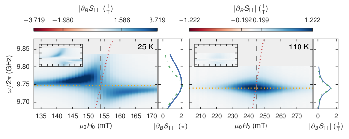
We measure the complex (phase sensitive) reflection scattering parameter $S_{11}$ around the resonance frequency of the cavity mode while applying a variable external magnetic field $H_{0}$ in the film plane. The applied probe power is chosen to be small ($0$ dBm) so that non-linear processes do not play a role. At this power, the number of photons excited in the cavity is approximately $N_{\mathrm{Ph}}=P/\left(\hbar\omega_{\mathrm{c}}\kappa_{\mathrm{c}}\right)=2\times 10^{13}$ and is several orders of magnitude lower than the minimum effective number of spins in the sample ($1\times 10^{17}$ for the highest analyzed temperature). In the microwave cabling connecting the cavity and the vector network analyzer, standing waves can form that cause a field independent background signal. In order to efficiently remove this background, we analyze the field derivative $\partial_{B}S_{11}=\frac{\partial S_{11}}{\partial(\mu_{0}H_{0})}$ as a function of $H_{0}$. Typical data for the absolute value of $\partial_{B}S_{11}$ is shown in Fig. 2 for two distinct temperatures. When the external magnetic field is adjusted to tune the FMR frequency $\omega_{\mathrm{FMR}}$ close to the unperturbed cavity frequency $\omega_{\mathrm{c}}$, the excitations of the magnetic system (magnons) and the microwave cavity (photons) start hybridizing with a signature in $S_{11}$ described by Eq. 1. For the case of strong coupling ($g_{\mathrm{eff}}\ >\kappa_{\mathrm{c}},\gamma_{\mathrm{s}}$) [Fig. 2 ($25\text{\,}\mathrm{K}$)], Eq. 1 describes a characteristic anti-crossing of the $H_{0}$-independent cavity mode and the $H_{0}$-dependent spin resonance. The splitting can be used to determine the coupling strength. In the weak coupling regime [Fig. 2 ($110\text{\,}\mathrm{K}$)], the cavity is only marginally disturbed. Here, the coupling strength can be determined by analyzing the change in the line width of the microwave cavity.[33] This case is equivalent to conventional FMR and therefore plotting the $S$ parameter at the cavity frequency as a function of the external field shows the typical FMR absorption line shape. Note that by taking the field derivative of $S_{11}$, the unperturbed cavity absorption peak vanishes (Fig. 2) as $\omega_{\mathrm{c}}$ is field independent.

Because we aim to observe the transition of the system from the weak coupling regime ($\gamma_{\mathrm{s}}>g_{\mathrm{eff}}$) to the strong coupling regime ($\kappa_{\mathrm{c}},\gamma_{\mathrm{s}}\leq g_{\mathrm{eff}}$), the approximate solutions for the extreme cases are not sufficient. The system has to be modeled by the complete reflection characteristic given by Eq. 1. To remove the field independent background of $S_{11}$, we first numerically calculate the magnetic field derivative of the complex $S_{11}$ parameter. We then perform a full 2D fit (i.e. all fits of all cuts at constant $H$ have shared parameter values) using the magnetic field derivative of Eq. 1 for every temperature. From this fit, we extract $M_{\mathrm{eff}}$, $g_{\mathrm{eff}}$, $\kappa_{\mathrm{c}}$ and $\gamma_{\mathrm{s}}$. The $g$-factor is fixed to $g=2$ over the whole temperature range based on Ref. 34 thereby reducing the number of free parameters further. The resulting fit is virtually indistinguishable from the data in Fig. 2. We therefore present the residual of the fit to the data in the insets on the same scale as the data. A vertical cut (dashed grey lines) of the 2D data and the fit is shown exemplarily for the static magnetic field corresponding to $\omega_{\mathrm{FMR}}=\omega_{\mathrm{c}}$. The 2D-fit is very good for high temperatures [Fig. 2 ($110\text{\,}\mathrm{K}$)], but the residuum shows some deviation of fit and data for low temperatures [Fig. 2 ($25\text{\,}\mathrm{K}$)]. We attribute this slight discrepancy to the presence of a second resonance line for our GdIG sample, which is apparent at low temperatures upon close examination. The second resonance might originate from spatial inhomogeneities in the sample. The data, the analysis scripts and results are publicly accessible under Ref. 35 for further analysis and evaluation.

We first discuss the effective magnetization $M_{\mathrm{eff}}$ extracted from the fitting procedure and displayed in the inset of Fig. 1 (red data points). The temperature evolution of the effective magnetization $M_{\mathrm{eff}}$ determined using FMR and the net magnetization $M$ measured by SQUID magnetometry agree well, indicating that the dominant anisotropy contribution in our GdIG thin film is indeed given by shape anisotropy. We therefore take $M=M_{\mathrm{eff}}$ in the following. The observed slight difference of $M$ and $M_{\mathrm{eff}}$ can be explained by a small increase of the $g$-factor with decreasing temperature as indicated in Ref. 34.

As central result, we confirm the scaling of the effective coupling rate $g_{\mathrm{eff}}$ with the magnetic moment (or magnetization). As mentioned above, we expect $g_{\mathrm{eff}}\propto\sqrt{M_{\mathrm{eff}}}$ in analogy to the paramagnetic case. Fig. 3 shows $g_{\mathrm{eff}}^{2}$ as a function of $M_{\mathrm{eff}}$  where a straight line indicates the expected scaling with $g_{\mathrm{eff}}=0$ at $M_{\mathrm{eff}}=0$. The data follows this behavior accurately over an order of magnitude of the magnetization. As noted above, for low temperatures (large magnetization) a second resonance is indicated that we do not fit separately. The fit therefore slightly overestimates the coupling in this regime which can also be seen in Fig. 3. From the slope, we can calculate the single spin – single photon coupling rate to $g_{\mathrm{s}}/2\pi=g_{0}/2\pi\left(\mu_{\mathrm{B}}\sqrt{3}/V\right)^{1/2}=$0.072\text{\,}\mathrm{Hz}$$ with the Bohr magneton $\mu_{\mathrm{B}}$ and the sample volume $V$ and assuming a spin 1/2 particle with a $g$-factor of 2. This value is in reasonable agreement with the values of $g_{\mathrm{s}}/2\pi=$0.043\text{\,}\mathrm{Hz}$$ determined for paramagnetic ensembles [9].

In order to coherently exchange excitations between a magnonic system such as GdIG and a photonic system, strong coupling (i.e. $\kappa_{\mathrm{c}},\gamma_{\mathrm{s}}\leq g_{\mathrm{eff}}$) is required. Fig. 4 displays the relaxation rate of the cavity $\kappa_{\mathrm{c}}$ and the spin system $\gamma_{\mathrm{s}}$ for comparison. The cavity decay rate $\kappa_{\mathrm{c}}$ should ideally be temperature independent but depends on the coupling of the feed line to the cavity.[32] As the temperature of the cavity is decreased, it thermally contracts slightly leading to a shift in resonance frequency and requires a change of the mechanical adjustment of the coupling mechanism. Hence, the decay rate of the cavity varies slightly with temperature. The mean value of $\kappa_{\mathrm{c}}$ is shown as green line in Fig. 4, while its standard deviation is depicted as green shaded area. The FMR line width, $\gamma_{\mathrm{s}}$ significantly increases towards $T_{\mathrm{comp}}$, in good agreement with reports in literature.[34] Finally, $g_{\mathrm{eff}}$ is plotted on the same scale and shows the increase towards low temperatures also shown in Fig. 3. Comparing the three rates, we find that the system is in the so-called high cooperativity regime ($\frac{g_{\mathrm{eff}}^{2}}{\kappa_{\mathrm{c}}\gamma_{\mathrm{s}}}>1$) for temperatures below $110\text{\,}\mathrm{K}$ (shaded region II in Fig. 3) and enters the strong coupling regime (region III) for liquid helium temperatures. By choosing a slightly larger sample size or specially shaped cavity modes[17], strong coupling and thus the coherent exchange of information between a 3D cavity and GdIG is feasible even at higher temperatures.

In conclusion, we investigated the magnon-photon coupling in a system consisting of a compensating ferrimagnet (GdIG) and a 3D microwave cavity by measuring and analyzing the full complex reflection spectra quantitatively. We control the magnetization of GdIG with temperature and extract the scaling of the coupling strength with the net magnetization of the sample. We thereby confirm the expected scaling behavior $g_{\mathrm{eff}}=g_{0}\sqrt{M}$ of the ferrimagnet–cavity system. This result proves that the description used for paramagnets is equally appropriate for exchange coupled spin systems. The coupling strength for a system with vanishing net remanent magnetization, as found in compensating ferrimagnets at the compensation point or for the exchange resonances in anti-ferromagnets, poses an interesting non-linear problem[36] that has yet to be addressed. In order to realize the transition from the strong to the weak coupling regime without modifying the sample or setup, we use a sample size that is just sufficient to reach the strong coupling regime. We emphasize, however, that strong coupling is easily accessible with GdIG / 3D microwave cavity system.

M. Harder acknowledges support from the NSERC MSFSS program. We gratefully acknowledge funding via the priority program Spin Caloric Transport (spinCAT), (Projects GO 944/4 and GR 1132/18), the priority program SPP 1601 (HU 1896/2-1) and the collaborative research center SFB 631 of the Deutsche Forschungsgemeinschaft.

References

- [1] Z.-L. Xiang, S. Ashhab, J. Q. You, and F. Nori, Reviews of Modern Physics 85, 623 (2013).
- [2] G. Kurizki, P. Bertet, Y. Kubo, K. Mølmer, D. Petrosyan, P. Rabl, and J. Schmiedmayer, Proceedings of the National Academy of Sciences 112, 3866 (2015).
- [3] A. Tkalčec, S. Probst, D. Rieger, H. Rotzinger, S. Wünsch, N. Kukharchyk, A. D. Wieck, M. Siegel, A. V. Ustinov, and P. Bushev, Physical Review B 90, 075112 (2014).
- [4] M. Tavis and F. W. Cummings, Physical Review 170, 379 (1968).
- [5] J. M. Fink, R. Bianchetti, M. Baur, M. Göppl, L. Steffen, S. Filipp, P. J. Leek, A. Blais, and A. Wallraff, Physical Review Letters 103, 083601 (2009).
- [6] A. Imamoğlu, Physical Review Letters 102, 083602 (2009).
- [7] I. Chiorescu, N. Groll, S. Bertaina, T. Mori, and S. Miyashita, Physical Review B 82, 024413 (2010).
- [8] Y. Kubo, F. R. Ong, P. Bertet, D. Vion, V. Jacques, D. Zheng, A. Dréau, J.-F. Roch, A. Auffeves, F. Jelezko, J. Wrachtrup, M. F. Barthe, P. Bergonzo, and D. Esteve, Physical Review Letters 105, 140502 (2010).
- [9] E. Abe, H. Wu, A. Ardavan, and J. J. L. Morton, Applied Physics Letters 98, 251108 (2011).
- [10] D. I. Schuster, A. P. Sears, E. Ginossar, L. DiCarlo, L. Frunzio, J. J. L. Morton, H. Wu, G. A. D. Briggs, B. B. Buckley, D. D. Awschalom, and R. J. Schoelkopf, Physical Review Letters 105, 140501 (2010).
- [11] P. Bushev, A. K. Feofanov, H. Rotzinger, I. Protopopov, J. H. Cole, C. M. Wilson, G. Fischer, A. Lukashenko, and A. V. Ustinov, Physical Review B 84, 060501 (2011).
- [12] C. W. Zollitsch, K. Mueller, D. P. Franke, S. T. B. Goennenwein, M. S. Brandt, R. Gross, and H. Huebl, Applied Physics Letters 107, 142105 (2015).
- [13] H. Huebl, C. W. Zollitsch, J. Lotze, F. Hocke, M. Greifenstein, A. Marx, R. Gross, and S. T. B. Goennenwein, Physical Review Letters 111, 127003 (2013).
- [14] X. Zhang, C.-l. Zou, L. Jiang, and H. X. Tang, Physical Review Letters 113, 156401 (2014).
- [15] Y. Tabuchi, S. Ishino, T. Ishikawa, R. Yamazaki, K. Usami, and Y. Nakamura, Physical Review Letters 113, 083603 (2014).
- [16] L. Bai, M. Harder, Y. P. Chen, X. Fan, J. Q. Xiao, and C.-M. Hu, Physical Review Letters 114, 227201 (2015).
- [17] N. Kostylev, M. Goryachev, and M. E. Tobar, Applied Physics Letters 108, 062402 (2016).
- [18] N. J. Lambert, J. A. Haigh, S. Langenfeld, A. C. Doherty, and A. J. Ferguson, Physical Review A 93, 021803 (2016).
- [19] X. Zhang, C.-l. Zou, N. Zhu, F. Marquardt, L. Jiang, and H. X. Tang, Nature Communications 6, 8914 (2015).
- [20] Y. Tabuchi, S. Ishino, A. Noguchi, T. Ishikawa, R. Yamazaki, K. Usami, and Y. Nakamura, Science 349, 405 (2015).
- [21] S. Klingler, H. Maier-Flaig, R. Gross, C.-M. Hu, H. Huebl, S. T. B. Goennenwein, and M. Weiler, Applied Physics Letters 109, 072402 (2016).
- [22] R. Hisatomi, A. Osada, Y. Tabuchi, T. Ishikawa, A. Noguchi, R. Yamazaki, K. Usami, and Y. Nakamura, Physical Review B 93, 174427 (2016).
- [23] Ö. O. Soykal and M. E. Flatté, Physical Review Letters 104, 077202 (2010).
- [24] Y. Cao, P. Yan, H. Huebl, S. T. B. Goennenwein, and G. E. W. Bauer, Physical Review B 91, 094423 (2015).
- [25] B. M. Yao, Y. S. Gui, Y. Xiao, H. Guo, X. S. Chen, W. Lu, C. L. Chien, and C.-M. Hu, Physical Review B 92, 184407 (2015).
- [26] C. Kittel, Introduction to Solid State Physics (John Wiley & Sons, New York, 1995).
- [27] G. F. Dionne, Magnetic Oxides (Springer US, Boston, MA, 2009).
- [28] G. F. Dionne and P. F. Tumelty, Journal of Applied Physics 50, 8257 (1979).
- [29] S. Geprägs, A. Kehlberger, F. D. Coletta, Z. Qiu, E.-J. Guo, T. Schulz, C. Mix, S. Meyer, A. Kamra, M. Althammer, H. Huebl, G. Jakob, Y. Ohnuma, H. Adachi, J. Barker, S. Maekawa, G. E. W. Bauer, E. Saitoh, R. Gross, S. T. B. Goennenwein, and M. Kläui, Nature Communications 7, 10452 (2016).
- [30] R. Pauthenet, Journal of Applied Physics 29, 253 (1958).
- [31] E. Sawatzky and E. Kay, Journal of Applied Physics 40, 1460 (1969).
- [32] H. Maier-Flaig, M. Harder, R. Gross, H. Huebl, and S. T. B. Goennenwein, Physical Review B 94, 054433 (2016).
- [33] P. F. Herskind, A. Dantan, J. P. Marler, M. Albert, and M. Drewsen, Nature Physics 5, 494 (2009).
- [34] B. A. Calhoun, J. Overmeyer, and W. V. Smith, Physical Review 107, 993 (1957).
- [35] H. Maier-Flaig, “GdIG temperature dependent coupling - 2D fits of the complex parameter,” (2017), doi: 10.17605/OSF.IO/D34DK.
- [36] Y. Mukai, H. Hirori, T. Yamamoto, H. Kageyama, and K. Tanaka, New Journal of Physics 18, 013045 (2016).