A Covert Queueing Channel in Round Robin Schedulers

AmirEmad Ghassami Ali Yekkehkhany and Negar Kiyavash ^†^†thanks: The authors are with the Department of Electrical and Computer Engineering, and Coordinated Science Laboratory, University of Illinois at Urbana-Champaign, Urbana, IL 61801, USA (email: {ghassam2,yekkehk2,kiyavash}@illinois.edu).

Abstract

We study a covert queueing channel (CQC) between two users sharing a round robin scheduler. Such a covert channel can arise when users share a resource such as a computer processor or a router arbitrated by a round robin policy. We present an information-theoretic framework to model and derive the maximum reliable data transmission rate, i.e., the capacity of this channel, for both noiseless and noisy setups. Our results show that seemingly isolated users can communicate with a high rate over the covert channel and demonstrate the possibility of significant information leakage and privacy threats brought by CQCs in round robin schedulers. Moreover, we propose practical finite-length code constructions, which achieve the capacity limit.

Index Terms:

Covert Queueing Channel, Round Robin Scheduler, Capacity Limit.

I Introduction

Shared resources among users in a system can lead to the occurrence of communication channels, which were not intended to exist in the system in the original design. Multiple users running on a computer who are using hardware resources such as CPU, storage, and multiple network streams flowing through a common router are examples of environments in which these channels can be created. Such channels are mainly used by a malicious user for gaining access to other users’ private information, and referred to as side channels [1, 2, 3]. For instance, the attacker can have an estimation of the features of the other users by analyzing their traffic. Previous work shows that through traffic analysis, the attacker can obtain various private information including exact schedules of real-time systems [4, 5], visited web sites [6], sent keystrokes [7], and even inferring spoken phrases in a voice-over-IP connection [8].

The coupling through shared resources can also be exploited for furtive communication among users. This type of channel is called a covert channel in the literature. Covert channels have typically been used by trusted insiders or malwares with access to secret information to leak it to untrusted outsiders [9, 10, 11, 12]. In most of the work in the area of covert channels, two users communicate by modulating the timings, and the receiver sees a noisy version of the transmitter’s inputs [13, 14, 15, 16, 17]. Also, there are many works devoted to the detection of such channels [18, 19, 20]. Unlike side channels, users in covert channels collaborate with each other and can agree on a specific usage pattern to efficiently utilize the features of the shared resource.

The focus of this paper is on the covert queueing channel (CQC), a special type of covert channel, that appears as a result of sharing a job scheduler among users. In a CQC, information is transmitted between the users through the delays that they experience when sending jobs to the shared scheduler. More specifically, due to the inter-dependencies between delays observed by users, if one user experiences delays in service, the user becomes aware that the other users are issuing jobs [14]. Different scheduling policies, such as first-come-first-served (FCFS), time-division-multiple-access (TDMA), round robin, etc., can be used for resource allocation among users. The optimal scheme for message transmission and the rate of communication between the users depends on the used policy.

For scheduling policies, there is a trade-off between throughput and security. For throughput, as long as the rates at which users request the shared resource are within the system’s capacity region, an effective scheduler should be able to respond to the users’ requests in a stable fashion. Such a scheduler is called a throughput optimal scheduler. From a throughput optimality point of view, TDMA scheduling policy decouples the serving times of the users and hence, causes significant delays in the service given to the users. Therefore, this policy is not throughput optimal. However, from the security point of view, since users’ delays are independent of each other in TDMA, this policy is the most secure scheduling policy [2]. The CQC created among users when the scheduler is FCFS is studied in detail in [21, 14]. Although this scheduler does not waste any resource and hence is throughput optimal, it allows users to communicate with an information rate as high as 0.8114 bits per time slot.

In this paper we focus on a round robin scheduler, which is another throughput optimal policy commonly used in computer processors and communication networks. Kadloor et al. [22] showed that when dealing with queueing side channels, round robin scheduling policy is privacy optimal within the class of work-conserving policies. We focus on covert channels created in this scheduler. We present an information-theoretic framework to describe and model the data transmission in this channel and calculate its capacity.

Our system model is depicted in Figure 1. In this model we have an encoder and a decoder user, represented by Alice and Bob, respectively. There is no direct communication channel between the users, but they share a round robin scheduler. Hence, the delays observed by users are correlated. Therefore, Alice can encode a message in her traffic pattern and Bob can estimate the message by estimating Alice’s traffic pattern via the delays he experiences. We show that users can communicate with an information rate of 0.6942 bits per time slot through the covert channel created between them in this system in the absence of noise. Additionally, we study the noisy version of this covert channel in which packets are dropped with a certain probability, and we compute the capacity as a function of packet drop probability.

Followings are the main contributions of this work.

•

We obtain the optimum signaling scheme for the CQC with round robin scheduler, and show that the capacity of the CQC is approximately 0.6942 bits per time slot (Section III).
•

We propose an optimal finite block length coding scheme both when codewords are of fixed and of variable lengths. Our results show that the rates of the proposed optimal coding schemes approach the capacity as the number of messages goes to infinity (Section IV).
•

We extend the model to a more realistic noisy case, and calculate the capacity for this case as well (Section V).

II System Model

We consider the system model depicted in Figure 1. In this model, a shared resource services jobs from two users, Alice and Bob, using round robin policy. In this depiction, each packet is marked by its arrival time. As shown in this figure, there is a feedback line from the shared resource to the users, which notifies them when their packet is served. This allows the users to infer the status of the head of their queue; that is, at each time, the users will be aware that which one of their packets will be served next.

Time is assumed to be discretized into slots, and the scheduler can serve one packet in each time slot. We follow the common convention that the packets arrive at the beginning of time slots and the departures occur at the end of time slots [23, 24]. Each user’s packets are buffered in a separate queue, and the round robin scheduler picks packets from the two queues as follows. In each time slot, three cases may happen: (a) If both users’ arrival queues are empty, the system remains idle and resumes scheduling in the next time slot. (b) If only one user’s queue has a packet, the current slot is given to that user, and the scheduler continues scheduling in the next time slot. (c) If both users have waiting packets, the scheduler always gives priority to a fixed user. That is, the current time slot is allocated to serve a packet from the user with higher priority, and the next time slot will be allocated to the other user. The system continues scheduling after both users have received service. Without loss of generality, we assume that the priority is always given to Bob in the sequel.

We assume both Alice and Bob send at most one packet per time slot. Thus, their packet stream can be modeled as a binary bit stream, where bit ‘1’ indicates a packet was sent, and bit ‘0’ indicates no packet was transmitted. Since the scheduler can serve at most one packet per time slot, the sum of users’ packet rates should be less than one for stability, that is, $\mathchar 28949_{\mathchar 28721}\mathchar 8235\mathchar 28949_{\mathchar 28722}\mathchar 12604\mathchar 28721$ , where $\mathchar 28949_{\mathchar 28721}$ and $\mathchar 28949_{\mathchar 28722}$ denote Alice and Bob’s packet rates, respectively. (See Appendix A for the proof of stability.)

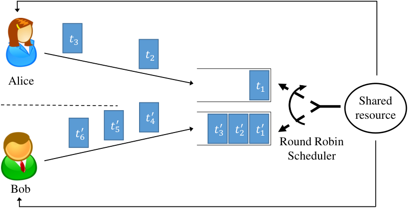
Refer to caption — Fig. 1: System Setup: Alice and Bob share a resource arbitrated in round robin fashion. Users get acknowledgments when their packets are served.

Figure 2 depicts an example of the scheduling in the system. In this and other such figures, Alice’s and Bob’s packets are shown by circled tip and regular arrows, respectively. For each user, the arrival stream, the head-of-the-queue stream and the departure stream are shown. Here, the arrival stream is the actual packet stream sent by the user, and the head-of-the-queue stream is the packets ready to be served at the head of the corresponding user’s queue. Therefore, at any given time slot, the head of the queue can be ‘1’ even though no packet has arrived in that slot. The downward streams in Figure 2(c) indicate the departure time of users’ packets. A packet is issued by both Alice and Bob in time slot 3. Since the priority is with Bob, his packet is processed in the same time slot, and Alice’s packet is delayed by one time slot. Hence, Alice’s head-of-the-queue stream contains a packet in both time slots 3 and 4. In Figure 2(b), the packet denoted by the gray dashed line indicates that it has been the same as its previous packet, which has been made to wait in the queue for one time slot to receive service in the next time slot. Alice’s packet is processed in time slot 4, causing a delay for Bob’s new packet sent in this time slot.

Suppose Alice aims to send message $\mathchar 29015$ drawn uniformly from the set $\{\mathchar 28721\mathchar 24891\mathchar 28722\mathchar 24891\dots\mathchar 24891\mathchar 29005\}$ . To this end, Alice encodes this message to a bit stream $\mathchar 29016^{\mathchar 29037}$ of length $\mathchar 29037$ , which is the codeword corresponding to message $\mathchar 29015$ . This codeword is sent out as a binary arrival stream $\mathchar 28993_{\mathchar 28993}^{\mathchar 29038}$ of length $\mathchar 29038$ . In the same $\mathchar 29038$ time slots, based on scheduling policy and both Alice’s and Bob’s packet arrivals, Bob receives a binary acknowledgment stream from the system, which is denoted by $\mathchar 28996_{\mathchar 28994}^{\mathchar 29038}$ . Finally, Bob transforms this stream to a bit stream $\mathchar 29017^{\mathchar 29037}$ which will be decoded to message $\hat{\mathchar 29015}$ . As a result, we have the following Markov chain:

\mathchar 29015\mathchar 12833\mathchar 29016^{\mathchar 29037}\mathchar 12833\mathchar 28993_{\mathchar 28993}^{\mathchar 29038}\mathchar 12833\mathchar 28996_{\mathchar 28994}^{\mathchar 29038}\mathchar 12833\mathchar 29017^{\mathchar 29037}\mathchar 12833\hat{\mathchar 29015}

(1)

The noise in the system is modeled as follows. The packets generated by either Alice or Bob may be dropped in the link between the users and the shared resource with probability $\mathchar 28942$ . Note that this noise can affect the transmissions in $\mathchar 29016^{\mathchar 29037}\mathchar 12833\mathchar 28993_{\mathchar 28993}^{\mathchar 29038}$ and $\mathchar 28993_{\mathchar 28993}^{\mathchar 29038}\mathchar 12833\mathchar 28996_{\mathchar 28994}^{\mathchar 29038}$ in Markov chain (1). In Section III we will obtain the optimum signaling scheme between Alice and Bob, and will show that using this scheme, noise will not affect the transmission $\mathchar 28993_{\mathchar 28993}^{\mathchar 29038}\mathchar 12833\mathchar 28996_{\mathchar 28994}^{\mathchar 29038}$ .

III Coding Theorem

In this section we obtain the optimum signaling scheme between the users and calculate the capacity of the introduced covert channel. The performance metric used in defining the capacity is the average error probability, defined as follows.

\mathchar 29008_{\mathchar 29029}\triangleq\mathchar 29008\delimiter 67273472\mathchar 29015\mathrel{{{{\mathchar 566\mathchar 61}}}}\hat{\mathchar 29015}\delimiter 84054785\mathchar 12349\mathchar 4944\displaylimits_{\mathchar 29037\mathchar 12349\mathchar 28721}^{\mathchar 29005}{{\mathchar 28721\over\mathchar 29005}}{\mathchar 29008}\delimiter 67273472\hat{\mathchar 29015}\mathrel{{{{\mathchar 566\mathchar 61}}}}\mathchar 29037\delimiter 69640972\mathchar 29015\mathchar 12349\mathchar 29037\delimiter 84054785\mathchar 314

Next, we define concepts required for the coding theory. These definitions are natural extensions of the classical definitions in information theory [13, 25, 26].

Definition 1.

An $\delimiter 67273472\mathchar 29038\mathchar 24891\mathchar 29005\mathchar 24891\mathchar 28943\delimiter 84054785$ -code consists of a codebook of size $\mathchar 29005$ with equiprobable binary codewords of average length $\mathchar 29038$ satisfying $\mathchar 29008_{\mathchar 29029}\mathchar 12820\mathchar 28943$ .

Definition 2.

The information transmission rate of a code is $\mathchar 29010\mathchar 12349\log\mathchar 29005\delimiter 68408078\mathchar 29038\mathchar 24891$ which is the amount of conveyed information normalized by the average number of used time slots¹¹ 1 Throughout the paper, all the logarithms are in base 2..

Definition 3.

A rate $\mathchar 29010$ is said to be achievable if there exists a sequence of $\delimiter 67273472\mathchar 29038\mathchar 24891\mathchar 29005\mathchar 24891\mathchar 28943_{\mathchar 29038}\delimiter 84054785$ -codes such that $\mathchar 28943_{\mathchar 29038}\mathchar 12833\mathchar 28720$ as $\mathchar 29038\mathchar 12833\mathchar 561$ .

Definition 4.

The channel capacity is the supremum achievable rate at which Alice can communicate through the covert channel with Bob.

We first obtain the optimum signaling scheme between the users, which maximizes the information transmission.

Lemma 1.

In the CQC in Figure 1, the maximum information transmission rate between the users is achieved when Bob’s head-of-the-queue bit stream is always equal to ‘1’.

See Appendix B for a proof.

The requirement that Bob should have a packet in his head-of-the-queue at all time slots does not mean that he has to send a packet in all time slots. It suffices for him to fix his queue length at some nonzero length, and whenever one of his packets is served, he generates a packet to ensure his queue length remains nonzero. This strategy allows him to keep the sum rate of arrivals from Alice and Bob less than 1 and keep the system stable.

As stated in the proof of Lemma 1, in an optimal signaling, Alice can signal two distinguishable patterns to Bob. These patterns require Alice to have either a ‘0’ or a ‘1’ in her head-of-the-queue stream. We will next demonstrate the arrival stream required for these head-of-the-queue streams.

For Alice to have a ‘0’ in her head-of-the-queue stream, assuming the queue is empty, she needs to idle for one time slot. Therefore, $\mathchar 28993_{\mathchar 28993}$ should contain a ‘0’. If Alice has a ‘1’ in her head-of-the-queue stream, two time slots are required for this signal to be transmitted (one for Bob’s packet and one for Alice’s). Therefore, $\mathchar 28993_{\mathchar 28993}$ should contain a ‘10’. Note that Alice should not send two packets in two consecutive time slots. This is because if Alice sends two (or more) packets in consecutive time slots, her next (or more) ‘0’(s) would disappear as her packets are accumulated in the queue. This is demonstrated in Example 1.

Fig. 2: (a) Arrival streams; (b) Head-of-the-queue streams; (c) Departure streams.

Example 1.

Assume that Alice’s queue is empty and she wants to transmit the bit stream $\mathchar 28721\mathchar 28721\mathchar 28720\mathchar 28721$ to Bob. If Alice sends ‘1’s in her message consecutively in each time slot (as depicted in Figure 3(a)), Bob would erroneously decode the message ‘111’. This is caused by the accumulation of packets in Alice’s queue, stemming from existence of a packet at the head of her queue before clearing the previous ‘1’. Figure 3(b) depicts the correct signaling by Alice.

Therefore, the optimum signaling scheme from Alice to Bob which maximizes the information transmission rate would be summarized as follows:

•

Signaling bit ‘1’: To signal bit ‘1’ in time slot $\mathchar 29038$ , Alice must have a head-of-the-queue packet at the beginning of the time slot. Recall that Bob has a ready-to-be-served packet in all time slots. Thus, round robin policy will serve Bob and Alice at time slots $\mathchar 29038$ and $\mathchar 29038\mathchar 8235\mathchar 28721$ , respectively. Therefore, when Bob receives service in a time slot but does not receive service in the next time slot, he decodes bit ‘1’.
•

Signaling bit ‘0’: To signal bit ‘0’ in time slot $\mathchar 29038$ , Alice must not have a head-of-the-queue packet at the beginning of the time slot. Because Bob has a packet which is ready to be serviced in the head of the queue in this time slot, he receives service at time slot $\mathchar 29038$ , and the scheduler resets for time slot $\mathchar 29038\mathchar 8235\mathchar 28721$ . As a result, at time slot $\mathchar 29038\mathchar 8235\mathchar 28721$ , Bob is served again. Therefore, if Bob receives service in two consecutive time slots, he decodes it as bit ‘0’.

This scheme implies the following lemma.

Lemma 2.

In the CQC in Figure 1, in the scheme with the maximum information transmission rate between the users, we have

{{\mathchar 29037\over\mathchar 29038}}\mathchar 12349{{\mathchar 28721\over\mathchar 28721\mathchar 8235\mathchar 29040}}\mathchar 24891

where $\mathchar 29040\mathchar 12349\mathchar 29008\delimiter 67273472\mathchar 29016\mathchar 12349\mathchar 28721\delimiter 84054785$ .

Proof.

According to the optimum signaling scheme, sending a bit ‘0’ and a bit ‘1’ require 1 and 2 time slots respectively. Therefore,

{{\mathchar 29037\over\mathchar 29038}}\mathchar 12349{{\mathchar 29037\over\mathchar 28722\mathchar 29040\mathchar 29037\mathchar 8235\delimiter 67273472\mathchar 28721\mathchar 8704\mathchar 29040\delimiter 84054785\mathchar 29037}}\mathchar 12349{{\mathchar 28721\over\mathchar 28721\mathchar 8235\mathchar 29040}}\mathchar 314

∎

Equipped with Lemma 2, we next calculate the capacity of the introduced covert channel.

Theorem 1.

The capacity of the introduced CQC in a shared round robin scheduler in Figure 1 is

\mathchar 28995\mathchar 12349\max_{\mathchar 28720\mathchar 12820\mathchar 29040\mathchar 12820\mathchar 28721}{{\mathchar 29032\delimiter 67273472\mathchar 29040\delimiter 84054785\over\mathchar 28721\mathchar 8235\mathchar 29040}}\mathchar 24891

(2)

where $\mathchar 29040$ is the probability of sending message bit ‘1’ by Alice and $\mathchar 29032\delimiter 67273472\mathchar 8705\delimiter 84054785$ is the binary entropy function.

The proof of Theorem 1 is presented in Appendix C. The maximum of (2) is approximately $\mathchar 28720\mathchar 314\mathchar 28726\mathchar 28729\mathchar 28724\mathchar 28722$ achieved at $\mathchar 29040\mathchar 12349{{\mathchar 28723\mathchar 8704\sqrt{\mathchar 28725}\over\mathchar 28722}}$ .

Fig. 3: Visualization of Example 1.

IV Finite-length Codeword Regime

We proposed an achievable scheme in the proof of Theorem 1; however, this scheme requires the value of $\mathchar 29038$ to tend to infinity to achieve the capacity. In this section we obtain the optimum coding schemes in finite-length codeword regime for communication in the introduced covert queueing channel. Our proposed schemes achieve information rates close to the capacity even with small codebooks.

As mentioned earlier, Alice encodes each message to a binary sequence and creates a codebook $\mathcal{\mathchar 28995}$ , known to both Alice and Bob. The codewords in the codebook could be all of the same or different lengths. In the following two subsections, we will consider both these scenarios and find the optimum codebook for the setting.

IV-A Variable-length Codewords

In this subsection, for any fixed number of messages $\mathchar 29005$ , we propose an algorithm which generates the optimum variable-length codebook, i.e., the list of codewords that results in maximum communication rate between the users. By Definition 1, the information rate at which Alice communicates with Bob could be computed as

\displaystyle\mathchar 29010\mathchar 12349{{\log\mathchar 29005\over{{\mathchar 28721\over\mathchar 29005}}\mathchar 4944\displaylimits_{\mathchar 29037\mathchar 12349\mathchar 28721}^{\mathchar 29037\mathchar 12349\mathchar 29005}\mathchar 29012_{\mathchar 29037}}}\mathchar 24891

(3)

where $\mathchar 29012_{\mathchar 29037}$ is the transmission time of the $\mathchar 29037$ -th codeword. As we discussed in Section II, in an optimum signaling scheme, transmission of bit ‘1’ takes two time slots, while bit ‘0’ requires one time slot. Denote the number of bits ‘0’ and ‘1’ in codebook $\mathcal{\mathchar 28995}$ by $\mathchar 29038_{\mathchar 28720}\delimiter 67273472\mathcal{\mathchar 28995}\delimiter 84054785$ and $\mathchar 29038_{\mathchar 28721}\delimiter 67273472\mathcal{\mathchar 28995}\delimiter 84054785$ , respectively. Therefore, $\mathchar 4944\displaylimits_{\mathchar 29037\mathchar 12349\mathchar 28721}^{\mathchar 29037\mathchar 12349\mathchar 29005}\mathchar 29012_{\mathchar 29037}\mathchar 12349\mathchar 28722\mathchar 29038_{\mathchar 28721}\delimiter 67273472\mathcal{\mathchar 28995}\delimiter 84054785\mathchar 8235\mathchar 29038_{\mathchar 28720}\delimiter 67273472\mathcal{\mathchar 28995}\delimiter 84054785$ , and (3) could be rewritten as

\displaystyle\mathchar 29010\mathchar 12349{{\mathchar 29005\log\mathchar 29005\over\mathchar 28722\mathchar 29038_{\mathchar 28721}\delimiter 67273472\mathcal{\mathchar 28995}\delimiter 84054785\mathchar 8235\mathchar 29038_{\mathchar 28720}\delimiter 67273472\mathcal{\mathchar 28995}\delimiter 84054785}}\mathchar 314

(4)

Given that $\mathchar 29005$ is a fixed given parameter, maximizing the rate is equivalent to searching for a codebook which achieves the minimum of the denominator in (4).

Fig. 4: A tree representation of the codewords. Codewords are the leaves of the tree. The cost of a codeword, defined to be its transmission time, is written in the boxes.

Our technique for finding the optimum codebook is as follows. We represent each codeword in the codebook by a leaf in a tree, as depicted in Figure 4. We define the cost of the codeword $\bar{\mathchar 29016}$ as the number of time slots required for transmission of this codeword, and denote it by $\mathchar 28945\delimiter 67273472\bar{\mathchar 29016}\delimiter 84054785$ . That is, $\mathchar 28945\delimiter 67273472\bar{\mathchar 29016}\delimiter 84054785\mathchar 12349\mathchar 28722\mathchar 29038_{\mathchar 28721}\delimiter 67273472\bar{\mathchar 29016}\delimiter 84054785\mathchar 8235\mathchar 29038_{\mathchar 28720}\delimiter 67273472\bar{\mathchar 29016}\delimiter 84054785$ , where $\mathchar 29038_{\mathchar 28720}\delimiter 67273472\bar{\mathchar 29016}\delimiter 84054785$ and $\mathchar 29038_{\mathchar 28721}\delimiter 67273472\bar{\mathchar 29016}\delimiter 84054785$ denote the number of bits ‘0’ and ‘1’ in $\bar{\mathchar 29016}$ , respectively. The numbers in boxes in Figure 4 denote the cost of each codeword. We call the resulting graph, the codeword tree. In this representation, for each node, the branch to the left (right) side, appends a 0 (1) to the codeword corresponding to that node. For example, if a vertex represents the bit stream $\mathchar 28720\mathchar 28720\mathchar 28721\mathchar 28720\mathchar 28721$ , its left and right children will represent codewords $\mathchar 28720\mathchar 28720\mathchar 28721\mathchar 28720\mathchar 28721\mathchar 28720$ and $\mathchar 28720\mathchar 28720\mathchar 28721\mathchar 28720\mathchar 28721\mathchar 28721$ , respectively. The reason we use the leaves of a tree for representing the codewords is to guarantee that the codewords are uniquely decodable [25].

Fig. 5: The maximum rates at which Alice can communicate with Bob versus the number of codewords for two cases of variable- and fixed-length codebooks.

Algorithm 1 describes how the $\mathchar 29005$ optimal codewords are selected from the tree. In this algorithm, we initialize the codebook to be $\{\mathchar 28720\mathchar 24891\mathchar 28721\}$ . In each iteration, one of the current codewords $\bar{\mathchar 29016}$ with minimum cost is replaced with its two children $\bar{\mathchar 29016}\mathchar 28720$ and $\bar{\mathchar 29016}\mathchar 28721$ . This procedure is repeated until all $\mathchar 29005$ codewords are obtained. As an example, the result of Algorithm 1 for $\mathchar 29005\mathchar 12349\mathchar 28726$ is depicted in Figure 4.

Algorithm 1 Finding the optimum variable-length codebook with

\mathchar 29005

codewords

1: Initialize

\mathcal{\mathchar 28995}\mathchar 12349\{\mathchar 28720\mathchar 24891\mathchar 28721\}

2: while

\delimiter 69640972\mathcal{\mathchar 28995}\delimiter 69640972\mathchar 12820\mathchar 29005

3: Find

\bar{\mathchar 29016}^{\mathchar 8707}\mathchar 12349\arg\min_{\bar{\mathchar 29016}\mathchar 12850\mathcal{\mathchar 28995}}\mathchar 28945\delimiter 67273472\bar{\mathchar 29016}\delimiter 84054785

\mathcal{\mathchar 28995}\mathchar 12349\mathcal{\mathchar 28995}\mathchar 8814\{\bar{\mathchar 29016}\}

\mathcal{\mathchar 28995}\mathchar 12349\mathcal{\mathchar 28995}\mathchar 8795\{\bar{\mathchar 29016}\mathchar 28720\}\mathchar 8795\{\bar{\mathchar 29016}\mathchar 28721\}

6: end while

7: Output

\mathcal{\mathchar 28995}

Theorem 2.

For a fixed given number of equiprobable messages, Algorithm 1 is optimal in the sense that it provides a codebook which maximizes the communication rate between the users.

A proof of Theorem 2 is presented in Appendix D.

The maximum rate at which Alice can communicate with Bob versus the number of codewords $\mathchar 29005$ , is depicted in Figure 5. The overall trend of the maximum communication rate increases as the number of codewords increases, and converges to the capacity. The following theorem formalizes this claim.

Theorem 3.

The information transmission rate of a codebook created by Algorithm 1 converges to the capacity of the covert channel as the number of messages goes to infinity.

A proof of Theorem 3 is presented in Appendix E.

IV-B Fixed-length Codeword

In many applications, using variable-length codewords is not desirable from the designer’s point of view. For example, in a noisy system, a variable-length scheme may lead to loss of synchronization between encoder and decoder. To obtain fixed-length codewords, all $\mathchar 29005$ codewords must be selected from the same level of the codeword tree. Such a constraint on choosing codewords can lead to reduction in information rate for a fixed number of messages, however, as we shall see, these codes can still achieve the capacity when the length of the codewords goes to infinity.

Algorithm 2 Finding the optimum fixed-length codebook with

\mathchar 29005

codewords

1: Initialize

\hat{\mathchar 29036}\mathchar 12349\delimiter 69616390\mathchar 29036\mathchar 29039\mathchar 29031\delimiter 67273472\mathchar 29005\delimiter 84054785\delimiter 86397703

2: for $\mathchar 29036\mathchar 12349\hat{\mathchar 29036}$ to $\mathchar 28722\hat{\mathchar 29036}$ do

\mathcal{\mathchar 28995}_{\mathchar 29036}

= Set of

\mathchar 29005

codewords with the least number of ‘0’s in the

\mathchar 29036

-th level of the codeword tree

\mathchar 28945\delimiter 67273472\mathcal{\mathchar 28995}_{\mathchar 29036}\delimiter 84054785\mathchar 12349\mathchar 29038_{\mathchar 28720}\delimiter 67273472\mathcal{\mathchar 28995}_{\mathchar 29036}\delimiter 84054785\mathchar 8235\mathchar 28722\mathchar 29038_{\mathchar 28721}\delimiter 67273472\mathcal{\mathchar 28995}_{\mathchar 29036}\delimiter 84054785

5: end for

\mathchar 29036^{\mathchar 8707}\mathchar 12349\arg\min_{\mathchar 29036}\mathchar 28945\delimiter 67273472\mathcal{\mathchar 28995}_{\mathchar 29036}\delimiter 84054785

7: Output

\mathcal{\mathchar 28995}_{\mathchar 29036^{\mathchar 8707}}

Our proposed approach for selecting the optimal fixed-length codebook for a given number of messages is presented in Algorithm 2. Denote the cost of a codebook with $\mathchar 28945\delimiter 67273472\mathcal{\mathchar 28995}\delimiter 84054785\mathchar 12349\mathchar 29038_{\mathchar 28720}\delimiter 67273472\mathcal{\mathchar 28995}\delimiter 84054785\mathchar 8235\mathchar 28722\mathchar 29038_{\mathchar 28721}\delimiter 67273472\mathcal{\mathchar 28995}\delimiter 84054785$ , which is the sum of the cost of its codewords. In Algorithm 2 first the optimum codebooks with the least number of ‘1’s should be chosen in each of the levels $\hat{\mathchar 29036}\mathchar 12349\delimiter 69616390\log\delimiter 67273472\mathchar 29005\delimiter 84054785\delimiter 86397703$ to $\mathchar 28722\hat{\mathchar 29036}$ . The optimal codebook is then the one with minimum cost among these created codebooks.

Theorem 4.

For a fixed given number of equiprobable messages, Algorithm 2 outputs the optimal fixed-length codebook.

A proof of Theorem 4 is presented in Appendix F.

As shown in Figure 5, using Algorithm 2 the overall trend of the maximum communication rate increases as the number of codewords increases, and converges to the capacity. The following theorem formalizes this claim.

Theorem 5.

The information transmission rate of a codebook created by Algorithm 2 converges to the capacity of the covert channel as the number of messages goes to infinity.

A proof of Theorem 5, is presented in Appendix E.

The maximum rate at which Alice can communicate with Bob versus the number of codewords $\mathchar 29005$ , in the case of using fixed-length codewords is depicted in Figure 5.

V Noisy Channel Case

In this section we consider the case where the channel between the users is noisy. The noise model is as follows. The packets generated by either Alice or Bob may be dropped in the link between the users and the shared resource with probability $\mathchar 28942$ . We start by investigating the effect of the noise on the CQC between the users. The following definition is required in our analysis.

Definition 5.

A Z-channel with parameter $\mathchar 28942$ is a discrete memoryless channel, in which ‘0’ is always transmitted error-free, but ‘1’ is flipped with probability $\mathchar 28942$ (Figure 6).

For the case of noisy channel, Lemma 1 again holds and hence, the signaling scheme proposed in Section III, achieves the maximum information transmission rate in the noisy channel as well. As discussed in Section III, Bob should keep his queue length positive at all time slots. If he keeps his queue length large enough, even if his packets are dropped in multiple time slots, he still has remaining ready to be served packets in his queue. Thus by keeping the probability of his queue length becoming zero arbitrary small, Bob can avoid dropped packets impacting the scheme. Therefore, although noise can affect the transmissions in $\mathchar 29016^{\mathchar 29037}\mathchar 12833\mathchar 28993_{\mathchar 28993}^{\mathchar 29038}$ in Markov chain (1), it will not influence the transmission $\mathchar 28993_{\mathchar 28993}^{\mathchar 29038}\mathchar 12833\mathchar 28996_{\mathchar 28994}^{\mathchar 29038}$ .

Fig. 6: Z-channel model of the covet channel with packet drops.

Lemma 3.

In the proposed optimum signaling scheme proposed in Section III, packet drops convert the channel between Alice and Bob to a Z-channel with parameter $\mathchar 28942$ .

Proof.

Noise does not affect the data transmission when Alice sends ‘0’ as she does not send any packets in this case. On the other hand, when Alice sends a packet to communicate bit ‘1’, this bit will change to ‘0’ if the packet is dropped, which happens with probability $\mathchar 28942$ . As stated in Section III, normally Alice should wait for one time slot after she sends a packet; however, when packet drops occur she does not need to wait for a time slot. Alice can always tell that a drop has occurred because she knows her queue length at the end of each time slot. Thus the aggregate effect of noise may be modeled as a Z-channel. ∎

Figure 6 shows the resulting Z-channel. Note that the channel is depicted between $\mathchar 29016$ and $\mathchar 29017$ in Markov chain (1), but the noise occurs between sequences $\mathchar 29016$ and $\mathchar 28993_{\mathchar 28993}$ .

In the noisy channel case, Lemma 2 will be modified as follows.

Lemma 4.

In the noisy CQC in Figure 1, in the scheme with the maximum information transmission rate between the users, we have

{{\mathchar 29037\over\mathchar 29038}}\mathchar 12349{{\mathchar 28721\over\delimiter 67273472\mathchar 28721\mathchar 8704\mathchar 29040\delimiter 84054785\mathchar 8235\mathchar 28942\mathchar 29040\mathchar 8235\mathchar 28722\delimiter 67273472\mathchar 28721\mathchar 8704\mathchar 28942\delimiter 84054785\mathchar 29040}}\mathchar 24891

where $\mathchar 29040\mathchar 12349\mathchar 29008\delimiter 67273472\mathchar 29016\mathchar 12349\mathchar 28721\delimiter 84054785$ .

Proof.

According to the optimum signaling scheme, sending a bit ‘0’ and a bit ‘1’ require 1 and 2 time slots, respectively. A bit ‘0’ can be a result of either a send ‘0’ or a flipped ‘1’. Therefore,

∎

Equipped with Lemmas 3 and 4, we next calculate the capacity of the introduced noisy covert channel.

Fig. 7: Capacity of the noisy CQC versus the drop probability

\mathchar 28942

Theorem 6.

The capacity of the noisy CQC between Alice and Bob with packet drop probability $\mathchar 28942$ in a shared round robin scheduler in Figure 1 is

\mathchar 28995\mathchar 12349\underset{\mathchar 28720\mathchar 12820\mathchar 29040\mathchar 12820\mathchar 28721}{\mathrm{\mathchar 29037\mathchar 29025\mathchar 29048}}{{\mathchar 29032\delimiter 67273472\delimiter 67273472\mathchar 28721\mathchar 8704\mathchar 28942\delimiter 84054785\mathchar 29040\delimiter 84054785\mathchar 8704\mathchar 29040\mathchar 29032\delimiter 67273472\mathchar 28942\delimiter 84054785\over\delimiter 67273472\mathchar 28721\mathchar 8704\mathchar 29040\delimiter 84054785\mathchar 8235\mathchar 28942\mathchar 29040\mathchar 8235\mathchar 28722\delimiter 67273472\mathchar 28721\mathchar 8704\mathchar 28942\delimiter 84054785\mathchar 29040}}\mathchar 24891

(5)

where $\mathchar 29040$ is the probability of sending message bit ‘1’ by Alice and $\mathchar 29032\delimiter 67273472\mathchar 8705\delimiter 84054785$ is the binary entropy function.

See Appendix G for a proof.

Figure 7 depicts the capacity of the noisy CQC versus the dropping probability $\mathchar 28942$ .

In the noisy setting, as mentioned earlier, synchronization between the encoder and decoder sides of the system may be lost. To prevent this from happening, users can use a fixed-length codebook such as the one presented in Subsection IV-B.

VI Conclusion

We studied a covert queueing channel between two users sharing a round robin scheduler. An information-theoretic framework was proposed to derive the capacity of this channel in both noisy and noiseless cases. We showed that in the noiseless case, an information rate as high as 0.6942 bits per time slot is achievable in this channel. Clearly this rate of transmission can lead to significant information leakage in a system and deserves special attention in high security systems. For the noisy case, where users’ packets may drop, we again analyzed the highest achievable information rate and obtained the capacity for different levels of noise. Moreover, we proposed practical finite-length code constructions, which asymptotically achieves the capacity limit.

Appendix A Proof of Stability

As mentioned in Section II, each user has a separate queue. Denote the queue length and the number of packet arrivals at each queue at time slot $\mathchar 29038$ by $\mathchar 29041_{\mathchar 29033}\delimiter 67273472\mathchar 29038\delimiter 84054785$ and $\mathchar 29025_{\mathchar 29033}\delimiter 67273472\mathchar 29038\delimiter 84054785$ , respectively. Let $\mathbb{\mathchar 28997}\delimiter 67482370\mathchar 29025_{\mathchar 29033}\delimiter 67273472\mathchar 29038\delimiter 84054785\delimiter 84267779\mathchar 12349\mathchar 28949_{\mathchar 29033}$ and $\mathbb{\mathchar 28997}\delimiter 67482370\mathchar 29025_{\mathchar 29033}^{\mathchar 28722}\delimiter 67273472\mathchar 29038\delimiter 84054785\delimiter 84267779\mathchar 12604\mathchar 561$ , where $\mathchar 29033\mathchar 12850\{\mathchar 28993\mathchar 24891\mathchar 28994\}$ signifies Alice or Bob. We assume the arrival processes of Alice and Bob are independent of each other and the system state. The system is stable if neither user’s queue length grows to infinity in the steady state of the system, as long as the arrivals are in the capacity region of the scheduler. Thus, it suffices to prove that the sum of the queue lengths is finite with probability one, which implies the stability of both queues. We use the Foster-Lyapunov theorem to prove this statement [27]. Denote the sum of the queue lengths with $\hat{\mathchar 29041}\delimiter 67273472\mathchar 29038\delimiter 84054785\mathchar 12349\mathchar 29041_{\mathchar 28993}\delimiter 67273472\mathchar 29038\delimiter 84054785\mathchar 8235\mathchar 29041_{\mathchar 28994}\delimiter 67273472\mathchar 29038\delimiter 84054785$ , and the sum of packet arrivals for Alice and Bob with $\hat{\mathchar 29025}\delimiter 67273472\mathchar 29038\delimiter 84054785\mathchar 12349\mathchar 29025_{\mathchar 28993}\delimiter 67273472\mathchar 29038\delimiter 84054785\mathchar 8235\mathchar 29025_{\mathchar 28994}\delimiter 67273472\mathchar 29038\delimiter 84054785$ . Note that $\mathbb{\mathchar 28997}\delimiter 67482370\hat{\mathchar 29025}\delimiter 67273472\mathchar 29038\delimiter 84054785\delimiter 84267779\mathchar 12349\mathchar 28949_{\mathchar 28993}\mathchar 8235\mathchar 28949_{\mathchar 28994}$ and the second moment of $\hat{\mathchar 29025}\delimiter 67273472\mathchar 29038\delimiter 84054785$ is finite. As long as a task is available in one of the two queues, the round robin scheduler serves a task; that is, the service rate is one packet per time slot. Thus $\hat{\mathchar 29041}$ evolves as

\hat{\mathchar 29041}\delimiter 67273472\mathchar 29038\mathchar 8235\mathchar 28721\delimiter 84054785\mathchar 12349\delimiter 67273472\hat{\mathchar 29041}\delimiter 67273472\mathchar 29038\delimiter 84054785\mathchar 8235\hat{\mathchar 29025}\delimiter 67273472\mathchar 29038\delimiter 84054785\mathchar 8704\mathchar 28721\delimiter 84054785_{\mathchar 8235}\mathchar 24891

where $\delimiter 67273472\mathchar 29048\delimiter 84054785_{\mathchar 8235}\triangleq\max\{\mathchar 29048\mathchar 24891\mathchar 28720\}$ .

Choose the Lyapunov function $\mathchar 29014\delimiter 67273472\hat{\mathchar 29041}\delimiter 67273472\mathchar 29038\delimiter 84054785\delimiter 84054785\mathchar 12349{{\hat{\mathchar 29041}^{\mathchar 28722}\delimiter 67273472\mathchar 29038\delimiter 84054785\over\mathchar 28722}}$ . Note that this choice of Lyapunov function satisfies the requirements of non-negativity, being equal to zero only at $\hat{\mathchar 29041}\mathchar 12349\mathchar 28720$ , and going to infinity as $\hat{\mathchar 29041}$ goes to infinity [28]. We show that the drift of this Lyapunov function is negative outside of a bounded region of the state space, and is positive and finite inside this bounded region, which implies that the system state is positive recurrent.

		$\displaystyle\mathchar 29014\delimiter 67273472\hat{\mathchar 29041}\delimiter 67273472\mathchar 29038\mathchar 8235\mathchar 28721\delimiter 84054785\delimiter 84054785\mathchar 8704\mathchar 29014\delimiter 67273472\hat{\mathchar 29041}\delimiter 67273472\mathchar 29038\delimiter 84054785\delimiter 84054785\big\delimiter 69640972\hat{\mathchar 29041}\delimiter 67273472\mathchar 29038\delimiter 84054785\mathchar 12349\mathchar 29041\delimiter 84267779$
		$\displaystyle\mathchar 12349\mathbb{\mathchar 28997}\delimiter 67482370{{\delimiter 67273472\mathchar 29041\mathchar 8235\hat{\mathchar 29025}\delimiter 67273472\mathchar 29038\delimiter 84054785\mathchar 8704\mathchar 28721\delimiter 84054785_{\mathchar 8235}^{\mathchar 28722}\mathchar 8704\mathchar 29041^{\mathchar 28722}\over\mathchar 28722}}\big\delimiter 69640972\mathchar 29041\delimiter 84267779$
		$\displaystyle\mathchar 12820\mathbb{\mathchar 28997}\delimiter 67482370{{\hat{\mathchar 29025}^{\mathchar 28722}\delimiter 67273472\mathchar 29038\delimiter 84054785\mathchar 8235\mathchar 28721\mathchar 8235\mathchar 28722\hat{\mathchar 29025}\delimiter 67273472\mathchar 29038\delimiter 84054785\mathchar 29041\mathchar 8704\mathchar 28722\mathchar 29041\mathchar 8704\mathchar 28722\hat{\mathchar 29025}\delimiter 67273472\mathchar 29038\delimiter 84054785\over\mathchar 28722}}\delimiter 84267779$
		$\displaystyle\mathchar 12820\mathbb{\mathchar 28997}\delimiter 67482370{{\hat{\mathchar 29025}^{\mathchar 28722}\delimiter 67273472\mathchar 29038\delimiter 84054785\mathchar 8235\mathchar 28721\mathchar 8704\mathchar 28722\hat{\mathchar 29025}\delimiter 67273472\mathchar 29038\delimiter 84054785\over\mathchar 28722}}\mathchar 8704\mathchar 28722\mathchar 29041\mathchar 8235\mathchar 28722\hat{\mathchar 29025}\delimiter 67273472\mathchar 29038\delimiter 84054785\mathchar 29041\delimiter 84267779$
		$\displaystyle\mathchar 12349\mathchar 29027\mathchar 8704\mathchar 28722\mathchar 29041\delimiter 67273472\mathchar 28721\mathchar 8704\mathchar 28949_{\mathchar 28993}\mathchar 8704\mathchar 28949_{\mathchar 28994}\delimiter 84054785\mathchar 24891$

where in the last equality, $\mathchar 29027$ is a constant because $\hat{\mathchar 29025}$ has bounded first and second moments. For $\mathchar 28949_{\mathchar 28993}\mathchar 8235\mathchar 28949_{\mathchar 28994}\mathchar 12604\mathchar 28721$ , the drift of the Lyapunov function is bounded by the constant $\mathchar 29027$ in the bounded set $\mathchar 28994\mathchar 12349\{\hat{\mathchar 29041}\ \delimiter 69640972\ \hat{\mathchar 29041}\mathchar 12820{{\mathchar 29027\over\mathchar 28722\delimiter 67273472\mathchar 28721\mathchar 8704\mathchar 28949_{\mathchar 28993}\mathchar 8704\mathchar 28949_{\mathchar 28994}\delimiter 84054785}}\}$ , and is negative in the complement set, $\mathchar 28994^{\mathchar 29027}$ . Therefore, with our queueing structure and round robin scheduler, the system is stable as long as $\mathchar 28949_{\mathchar 28993}\mathchar 8235\mathchar 28949_{\mathchar 28994}\mathchar 12604\mathchar 28721$ .

Appendix B Proof of Lemma 1

Suppose Bob’s head-of-the-queue stream contains a ‘1’ followed by $\mathchar 29044$ ‘0’s. During these $\mathchar 29044\mathchar 8235\mathchar 28721$ bits, if Alice’s head-of-the-queue is equal to $\mathchar 29044\mathchar 8235\mathchar 28721$ consecutive ‘1’s, $\mathchar 28996_{\mathchar 28994}$ will contain a ‘1’ followed by $\mathchar 29044\mathchar 8235\mathchar 28721$ ‘0’s; otherwise, it will contain a ‘1’ followed by $\mathchar 29044$ ‘0’s. Therefore, denoting the probability of the event that Alice’s head-of-the-queue is equal to $\mathchar 29044\mathchar 8235\mathchar 28721$ consecutive ‘1’s by $\mathchar 29040_{\mathchar 29044\mathchar 8235\mathchar 28721}$ , there are two distinguishable outputs for Bob, received on average in $\delimiter 67273472\mathchar 29044\mathchar 8235\mathchar 28721\delimiter 84054785\delimiter 67273472\mathchar 28721\mathchar 8704\mathchar 29040_{\mathchar 29044\mathchar 8235\mathchar 28721}\delimiter 84054785\mathchar 8235\delimiter 67273472\mathchar 29044\mathchar 8235\mathchar 28722\delimiter 84054785\mathchar 29040_{\mathchar 29044\mathchar 8235\mathchar 28721}\mathchar 12349\delimiter 67273472\mathchar 29044\mathchar 8235\mathchar 28721\delimiter 84054785\mathchar 8235\mathchar 29040_{\mathchar 29044\mathchar 8235\mathchar 28721}$ time slots, which gives the information transmission rate of

{{\log\mathchar 28722\over\delimiter 67273472\mathchar 29044\mathchar 8235\mathchar 28721\delimiter 84054785\mathchar 8235\mathchar 29040_{\mathchar 29044\mathchar 8235\mathchar 28721}}}\mathchar 24891

which regardless of the value for $\mathchar 29040_{\mathchar 29044\mathchar 8235\mathchar 28721}$ , is maximized when $\mathchar 29044\mathchar 12349\mathchar 28720$ . Therefore, the maximum information transmission rate between the users is achieved when Bob’s head-of-the-queue bit stream is always equal to ‘1’.

Appendix C Proof of Theorem 1

The proof consists of achievability and converse arguments.
Converse: For the CQC in a shared round robin scheduler with service rate 1 depicted in Figure 1, any code consisting of a codebook of $\mathchar 29005$ equiprobable binary codewords, where messages take on average $\mathchar 29038$ time slots to be received, satisfies

	$\displaystyle{{\mathchar 28721\over\mathchar 29038}}\log{\mathchar 29005}$	$\displaystyle\stackrel{{\scriptstyle\delimiter 67273472\mathchar 29025\delimiter 84054785}}{{\mathchar 12349}}{{\mathchar 28721\over\mathchar 29038}}\mathchar 29000\delimiter 67273472\mathchar 29015\delimiter 84054785\mathchar 12349{{\mathchar 28721\over\mathchar 29038}}\mathchar 29000\delimiter 67273472\mathchar 29016^{\mathchar 29037}\delimiter 84054785\mathchar 12820{{\mathchar 28721\over\mathchar 29038}}\mathchar 4944\displaylimits_{\mathchar 29033\mathchar 12349\mathchar 28721}^{\mathchar 29037}\mathchar 29000\delimiter 67273472\mathchar 29016_{\mathchar 29033}\delimiter 84054785$
		$\displaystyle\mathchar 12820\max_{\mathchar 29008_{\mathchar 29016}}{{\mathchar 29037\over\mathchar 29038}}\mathchar 29000\delimiter 67273472\mathchar 29016\delimiter 84054785\mathchar 12820\max_{\mathchar 28720\mathchar 12820\mathchar 29040\mathchar 12820\mathchar 28721}{{\mathchar 29037\over\mathchar 29038}}\mathchar 29032\delimiter 67273472\mathchar 29040\delimiter 84054785\mathchar 24891$

\mathchar 28995\mathchar 12820\max_{\mathchar 28720\mathchar 12820\mathchar 29040\mathchar 12820\mathchar 28721}{{\mathchar 29032\delimiter 67273472\mathchar 29040\delimiter 84054785\over\mathchar 28721\mathchar 8235\mathchar 29040}}\mathchar 314

Achievability: We fix a Bernoulli distribution $\mathchar 29008$ with parameter $\mathchar 29040^{\mathchar 8707}$ , where

\displaystyle\mathchar 29040^{\mathchar 8707}\mathchar 12349\arg\max_{\mathchar 29040\mathchar 12850\delimiter 67482370\mathchar 28720\mathchar 24891\mathchar 28721\delimiter 84267779}{{\mathchar 29032\delimiter 67273472\mathchar 29040\delimiter 84054785\over\mathchar 28721\mathchar 8235\mathchar 29040}}\mathchar 24891

and generate a binary codebook $\mathcal{\mathchar 28995}$ containing i.i.d. sequences of length $\mathchar 29037$ drawn according to $\mathchar 29008$ , where $\mathchar 29037\mathchar 12349{{\mathchar 29038\over\mathchar 28721\mathchar 8235\mathchar 29040^{\mathchar 8707}}}$ . A standard typicality argument [25, Chapter 3], shows that as $\mathchar 29038$ goes to infinity, we can have $\mathchar 28722^{\mathchar 29000\delimiter 67273472\mathchar 29016^{\mathchar 29037}\delimiter 84054785}\mathchar 12349\mathchar 28722^{\mathchar 29037\mathchar 29032\delimiter 67273472\mathchar 29040^{\mathchar 8707}\delimiter 84054785}$ distinct codewords in $\mathcal{\mathchar 28995}$ .

In order to send a bit ‘1’, Alice sends a packet and then idles for one time slot. To send a bit ‘0’, she just idles for one time slot. Thus, each message on average takes $\mathchar 28722\mathchar 29037\mathchar 29040^{\mathchar 8707}\mathchar 8235\mathchar 29037\delimiter 67273472\mathchar 28721\mathchar 8704\mathchar 29040^{\mathchar 8707}\delimiter 84054785\mathchar 12349\mathchar 29038$ time slots to be transmitted. At the same time, Bob keeps his head of the queue always full. Since this is a noiseless channel, the error will be zero. Therefore,

\mathchar 28995\mathchar 12821{{\log\mathchar 28722^{\mathchar 29037\mathchar 29032\delimiter 67273472\mathchar 29040^{\mathchar 8707}\delimiter 84054785}\over\mathchar 29038}}\mathchar 12349{{\mathchar 29037\mathchar 29032\delimiter 67273472\mathchar 29040^{\mathchar 8707}\delimiter 84054785\over\mathchar 29037\delimiter 67273472\mathchar 28721\mathchar 8235\mathchar 29040^{\mathchar 8707}\delimiter 84054785}}\mathchar 12349{{\mathchar 29032\delimiter 67273472\mathchar 29040^{\mathchar 8707}\delimiter 84054785\over\mathchar 28721\mathchar 8235\mathchar 29040^{\mathchar 8707}}}\mathchar 12349\max_{\mathchar 28720\mathchar 12820\mathchar 29040\mathchar 12820\mathchar 28721}{{\mathchar 29032\delimiter 67273472\mathchar 29040\delimiter 84054785\over\mathchar 28721\mathchar 8235\mathchar 29040}}\mathchar 314

The achievability and converse parts above, complete the proof of the coding theorem.

Appendix D Proof of Theorem 2

We show that Algorithm 1 minimizes the sum of costs of codewords which is $\mathchar 28722\mathchar 29038_{\mathchar 28721}\delimiter 67273472\mathcal{\mathchar 28995}\delimiter 84054785\mathchar 8235\mathchar 29038_{\mathchar 28720}\delimiter 67273472\mathcal{\mathchar 28995}\delimiter 84054785$ .

We note that, replacing codeword $\bar{\mathchar 29016}$ with cost $\mathchar 28945\delimiter 67273472\bar{\mathchar 29016}\delimiter 84054785$ results in two codewords $\bar{\mathchar 29016}\mathchar 28720$ and $\bar{\mathchar 29016}\mathchar 28721$ with costs $\mathchar 28945\delimiter 67273472\bar{\mathchar 29016}\delimiter 84054785\mathchar 8235\mathchar 28721$ and $\mathchar 28945\delimiter 67273472\bar{\mathchar 29016}\delimiter 84054785\mathchar 8235\mathchar 28722$ , respectively. As a result, replacing codeword $\bar{\mathchar 29016}$ with its two children causes additional cost of $\mathchar 28945\delimiter 67273472\bar{\mathchar 29016}\delimiter 84054785\mathchar 8235\mathchar 28723$ , and an additional codeword to the codebook. Therefore, since the added cost is increasing in $\mathchar 28945\delimiter 67273472\bar{\mathchar 29016}\delimiter 84054785$ , to obtain the optimal codebook in a step, it suffices to replace the minimum cost codeword by its children.

Suppose Algorithm 1 outputs codebook $\mathcal{\mathchar 28995}_{\mathchar 28721}$ . To prove the claim by contradiction, suppose the codebook $\mathcal{\mathchar 28995}_{\mathchar 28722}$ resulted from another algorithm is optimum where both $\mathcal{\mathchar 28995}_{\mathchar 28721}$ and $\mathcal{\mathchar 28995}_{\mathchar 28722}$ have $\mathchar 29005$ codewords. We first find the subtree which is common between $\mathcal{\mathchar 28995}_{\mathchar 28721}$ and $\mathcal{\mathchar 28995}_{\mathchar 28722}$ , which implies that two algorithms are equivalent until, say, step $\mathchar 29037$ . From that step, all the replacements are different in two algorithms. The first replacement in Algorithm 1 gives a smaller cost (because we assumed to choose the minimum cost replacement). For the next replacement in step $\mathchar 29037\mathchar 8235\mathchar 28721$ , Algorithm 1 had the option of the other algorithm’s replacement in step $\mathchar 29037$ , yet it did not choose that. This means that again a better replacement was possible. Adding this to the fact that the costs of children of a codeword is larger than its own cost, concludes that the replacement in step $\mathchar 29037\mathchar 8235\mathchar 28721$ for Algorithm 1 was also a better choice. This reasoning applies to all steps in which two algorithms are different and concludes that $\mathcal{\mathchar 28995}_{\mathchar 28722}$ cannot be optimum.

Appendix E Proof of Theorems 3 and 5

In this appendix, we show that the information transmission rate of our proposed optimum codebooks created by Algorithms 1 and 2 converge to the capacity of the covert channel as the number of messages goes to infinity. We prove that the information rate of another non-optimum codebook with rate lower than the rates of both aforementioned codebooks achieves the capacity.

Consider a codebook with fixed-length codewords from the $\mathchar 29036$ -th level of the codeword tree. We choose each codeword to have exactly $\delimiter 69608196\mathchar 29036\mathchar 29040\delimiter 86389509$ bits ‘1’, where the parameter $\mathchar 29040\mathchar 12850\delimiter 67482370\mathchar 28720\mathchar 24891\mathchar 28721\delimiter 84267779$ can be selected in a manner to maximize the information rate. Such a codebook consists of $\mathchar 29005\mathchar 12349{{\mathchar 29036}\choose{\delimiter 69608196\mathchar 29036\mathchar 29040\delimiter 86389509}}$ messages all of which have equal transmission time $\mathchar 28722\mathchar 8706\delimiter 69608196\mathchar 29036\mathchar 29040\delimiter 86389509\mathchar 8235\delimiter 67273472\mathchar 29036\mathchar 8704\delimiter 69608196\mathchar 29036\mathchar 29040\delimiter 86389509\delimiter 84054785$ . We show that the information rate of this codebook asymptotically converges to the capacity as $\mathchar 29036$ (or equivalently the number of messages) goes to infinity. From Definition 1, we have

	$\displaystyle\max_{\mathchar 29040}\lim_{\mathchar 29038\mathchar 12833\mathchar 561}{{\log{{\mathchar 29036}\choose{\delimiter 69608196\mathchar 29036\mathchar 29040\delimiter 86389509}}\over\mathchar 29038}}$	$\displaystyle\overset{\delimiter 67273472\mathchar 29025\delimiter 84054785}{\mathchar 12349}\max_{\mathchar 29040}\lim_{\mathchar 29036\mathchar 12833\mathchar 561}{{\mathchar 29036\mathchar 8705\mathchar 29032\delimiter 67273472{{\delimiter 69608196\mathchar 29036\mathchar 29040\delimiter 86389509\over\mathchar 29036}}\delimiter 84054785\mathchar 8235\mathchar 29039\delimiter 67273472\mathchar 29036\delimiter 84054785\over\mathchar 29036\mathchar 8235\delimiter 69608196\mathchar 29036\mathchar 29040\delimiter 86389509}}$
		$\displaystyle\overset{\delimiter 67273472\mathchar 29026\delimiter 84054785}{\mathchar 12349}\max_{\mathchar 29040}{{\mathchar 29032\delimiter 67273472\mathchar 29040\delimiter 84054785\over\mathchar 28721\mathchar 8235\mathchar 29040}}\mathchar 12349\mathchar 28995\mathchar 24891$

where $\mathchar 29038\mathchar 12349\mathchar 29036\mathchar 8235\delimiter 69608196\mathchar 29036\mathchar 29040\delimiter 86389509$ , $\delimiter 67273472\mathchar 29025\delimiter 84054785$ follows because using Stirling’s approximation it can be shown that $\log{{\mathchar 29036}\choose{\mathchar 29035}}\mathchar 12349\mathchar 29036\mathchar 8705\mathchar 29032\delimiter 67273472{{\mathchar 29035\over\mathchar 29036}}\delimiter 84054785\mathchar 8235\mathchar 29039\delimiter 67273472\mathchar 29036\delimiter 84054785$ , $\delimiter 67273472\mathchar 29026\delimiter 84054785$ holds since the binary entropy function $\mathchar 29032\delimiter 67273472\mathchar 8705\delimiter 84054785$ is continuous, and the last equality follows from Theorem 1.

Appendix F Proof of Theorem 4

It suffices to show that the best rate is contained in the search range of $\mathchar 29036\mathchar 12349\hat{\mathchar 29036}$ to $\mathchar 28722\hat{\mathchar 29036}$ .

First, we note that if $\mathchar 29036\mathchar 12604\hat{\mathchar 29036}$ , then $\mathchar 28722^{\mathchar 29036}\mathchar 12604\mathchar 29005$ , which implies that there is not a sufficient number of codewords in level $\mathchar 29036$ to cover all messages. On the other hand, since $\mathchar 29036\mathchar 12604{{\mathchar 28945\delimiter 67273472\mathcal{\mathchar 28995}_{\mathchar 29036}\delimiter 84054785\over\mathchar 29005}}\mathchar 12604\mathchar 28722\mathchar 29036$ , we have

{{\log\mathchar 29005\over\mathchar 28722\mathchar 29036}}\mathchar 12604\mathchar 29010_{\mathchar 29036}\mathchar 12604{{\log\mathchar 29005\over\mathchar 29036}}\mathchar 24891

where $\mathchar 29010_{\mathchar 29036}$ is the information rate of the optimum codebook at level $\mathchar 29036$ . Therefore, for all $\mathchar 29036\mathchar 12606\mathchar 28722\hat{\mathchar 29036}$ ,

\mathchar 29010_{\mathchar 29036}\mathchar 12604{{\log\mathchar 29005\over\mathchar 29036}}\mathchar 12604{{\log\mathchar 29005\over\mathchar 28722\hat{\mathchar 29036}}}\mathchar 12604\mathchar 29010_{\hat{\mathchar 29036}}\mathchar 314

In other words, for all $\mathchar 29036\mathchar 12606\mathchar 28722\hat{\mathchar 29036}$ the optimum information rate is less than the optimum information rate of $\mathcal{\mathchar 28995}_{\hat{\mathchar 29036}}$ . This implies that there is no need to check any level lower than $\hat{\mathchar 29036}$ .

Appendix G Proof of Theorem 6

	$\displaystyle\displaystyle{{\mathchar 28721\over\mathchar 29038}}\log{\mathchar 29005}$
		$\displaystyle\mathchar 12349{{\mathchar 28721\over\mathchar 29038}}\mathchar 29001\delimiter 67273472\mathchar 29015\mathchar 24635\hat{\mathchar 29015}\delimiter 84054785\mathchar 8235{{\mathchar 28721\over\mathchar 29038}}\mathchar 29000\delimiter 67273472\mathchar 29015\delimiter 69640972\hat{\mathchar 29015}\delimiter 84054785$
		$\displaystyle\overset{\delimiter 67273472\mathchar 29026\delimiter 84054785}{\mathchar 12820}{{\mathchar 28721\over\mathchar 29038}}\mathchar 29001\delimiter 67273472\mathchar 29015\mathchar 24635\hat{\mathchar 29015}\delimiter 84054785\mathchar 8235\mathchar 28943_{\mathchar 29038}$
		$\displaystyle\overset{\delimiter 67273472\mathchar 29027\delimiter 84054785}{\mathchar 12820}{{\mathchar 28721\over\mathchar 29038}}\mathchar 29001\delimiter 67273472\mathchar 29016^{\mathchar 29037}\mathchar 24635\mathchar 29017^{\mathchar 29037}\delimiter 84054785\mathchar 8235\mathchar 28943_{\mathchar 29038}\mathchar 24891$

where $\delimiter 67273472\mathchar 29025\delimiter 84054785$ holds because $\mathchar 29015$ is a uniform random variable over the message set $\{\mathchar 28721\mathchar 24891\mathchar 314\mathchar 314\mathchar 314\mathchar 24891\mathchar 29005\}$ , $\delimiter 67273472\mathchar 29026\delimiter 84054785$ follows from Fano’s inequality with $\mathchar 28943_{\mathchar 29038}\mathchar 12349{{\mathchar 28721\over\mathchar 29038}}\delimiter 67273472\mathchar 29000\delimiter 67273472\mathchar 29008_{\mathchar 29029}\delimiter 84054785\mathchar 8235\mathchar 29008_{\mathchar 29029}\log_{\mathchar 28722}{\delimiter 67273472\mathchar 29005\mathchar 8704\mathchar 28721\delimiter 84054785}\delimiter 84054785$ , and $\delimiter 67273472\mathchar 29027\delimiter 84054785$ follows from application of data processing inequality to the Markov chain in (1).

Since the Z-channel model is memoryless,

\mathchar 29001\delimiter 67273472\mathchar 29016^{\mathchar 29037}\mathchar 24635\mathchar 29017^{\mathchar 29037}\delimiter 84054785\mathchar 12820\mathchar 4944\displaylimits_{\mathchar 29033\mathchar 12349\mathchar 28721}^{\mathchar 29037}\mathchar 29001\delimiter 67273472\mathchar 29016_{\mathchar 29033}\mathchar 24635\mathchar 29017_{\mathchar 29033}\delimiter 84054785\mathchar 314

Therefore,

\displaystyle\displaystyle{{\mathchar 28721\over\mathchar 29038}}\log{\mathchar 29005}

\displaystyle\mathchar 12820\mathchar 4944\displaylimits_{\mathchar 29033\mathchar 12349\mathchar 28721}^{\mathchar 29037}{{\mathchar 28721\over\mathchar 29038}}\mathchar 29001\delimiter 67273472\mathchar 29016_{\mathchar 29033}\mathchar 24635\mathchar 29017_{\mathchar 29033}\delimiter 84054785\mathchar 8235\mathchar 28943_{\mathchar 29038}\mathchar 12820\max_{\mathchar 29008_{\mathchar 29016}}{{\mathchar 29037\over\mathchar 29038}}\mathchar 29001\delimiter 67273472\mathchar 29016\mathchar 24635\mathchar 29017\delimiter 84054785\mathchar 8235\mathchar 28943_{\mathchar 29038}\mathchar 314

By Lemma 4, in the scheme with the maximum information transmission rate between Alice and Bob, we have ${{\mathchar 29037\over\mathchar 29038}}\mathchar 12349{{\mathchar 28721\over\delimiter 67273472\mathchar 28721\mathchar 8704\mathchar 29040\delimiter 84054785\mathchar 8235\mathchar 28942\mathchar 29040\mathchar 8235\mathchar 28722\delimiter 67273472\mathchar 28721\mathchar 8704\mathchar 28942\delimiter 84054785\mathchar 29040}}$ . Also, we note that

\displaystyle\mathchar 29001\delimiter 67273472\mathchar 29016\mathchar 24635\mathchar 29017\delimiter 84054785\mathchar 12349

Therefore, we have

\displaystyle\displaystyle{{\mathchar 28721\over\mathchar 29038}}\log{\mathchar 29005}\mathchar 12820\max_{\mathchar 28720\mathchar 12820\mathchar 29040\mathchar 12820\mathchar 28721}{{\mathchar 29032\delimiter 67273472\delimiter 67273472\mathchar 28721\mathchar 8704\mathchar 28942\delimiter 84054785\mathchar 29040\delimiter 84054785\mathchar 8704\mathchar 29040\mathchar 29032\delimiter 67273472\mathchar 28942\delimiter 84054785\over\delimiter 67273472\mathchar 28721\mathchar 8704\mathchar 29040\delimiter 84054785\mathchar 8235\mathchar 28942\mathchar 29040\mathchar 8235\mathchar 28722\delimiter 67273472\mathchar 28721\mathchar 8704\mathchar 28942\delimiter 84054785\mathchar 29040}}\mathchar 8235\mathchar 28943_{\mathchar 29038}\mathchar 314

As $\mathchar 29038$ goes to infinity, $\mathchar 28943_{\mathchar 29038}\mathchar 12833\mathchar 28720$ , and we have

\displaystyle\mathchar 28995\mathchar 12820\max_{\mathchar 28720\mathchar 12820\mathchar 29040\mathchar 12820\mathchar 28721}{{\mathchar 29032\delimiter 67273472\delimiter 67273472\mathchar 28721\mathchar 8704\mathchar 28942\delimiter 84054785\mathchar 29040\delimiter 84054785\mathchar 8704\mathchar 29040\mathchar 29032\delimiter 67273472\mathchar 28942\delimiter 84054785\over\delimiter 67273472\mathchar 28721\mathchar 8704\mathchar 29040\delimiter 84054785\mathchar 8235\mathchar 28942\mathchar 29040\mathchar 8235\mathchar 28722\delimiter 67273472\mathchar 28721\mathchar 8704\mathchar 28942\delimiter 84054785\mathchar 29040}}\mathchar 314

Achievability: Fix a Bernoulli distribution $\mathchar 29008$ with parameter $\mathchar 29040^{\mathchar 8707}$ , where

\displaystyle\mathchar 29040^{\mathchar 8707}\mathchar 12349\arg\max_{\mathchar 28720\mathchar 12820\mathchar 29040\mathchar 12820\mathchar 28721}{{\mathchar 29032\delimiter 67273472\delimiter 67273472\mathchar 28721\mathchar 8704\mathchar 28942\delimiter 84054785\mathchar 29040\delimiter 84054785\mathchar 8704\mathchar 29040\mathchar 29032\delimiter 67273472\mathchar 28942\delimiter 84054785\over\delimiter 67273472\mathchar 28721\mathchar 8704\mathchar 29040\delimiter 84054785\mathchar 8235\mathchar 28942\mathchar 29040\mathchar 8235\mathchar 28722\delimiter 67273472\mathchar 28721\mathchar 8704\mathchar 28942\delimiter 84054785\mathchar 29040}}\mathchar 24891

and generate a binary codebook $\mathcal{\mathchar 28995}$ containing $\mathchar 28722^{\mathchar 29037\mathchar 29010}$ i.i.d. sequences of length $\mathchar 29037$ , drawn according to $\mathchar 29008$ , where $\mathchar 29037\mathchar 12349\mathchar 29038\delimiter 68408078\delimiter 67482370\delimiter 67273472\mathchar 28721\mathchar 8704\mathchar 29040^{\mathchar 8707}\delimiter 84054785\mathchar 8235\mathchar 28942\mathchar 29040^{\mathchar 8707}\mathchar 8235\mathchar 28722\delimiter 67273472\mathchar 28721\mathchar 8704\mathchar 28942\delimiter 84054785\mathchar 29040^{\mathchar 8707}\delimiter 84267779$ .

In order to send a bit ‘1’, Alice sends a packet and then idles for one time slot. To send a bit ‘0’, she just idles for one time slot. Thus, each message on average takes $\mathchar 29037\delimiter 67482370\delimiter 67273472\mathchar 28721\mathchar 8704\mathchar 29040^{\mathchar 8707}\delimiter 84054785\mathchar 8235\mathchar 28942\mathchar 29040^{\mathchar 8707}\mathchar 8235\mathchar 28722\delimiter 67273472\mathchar 28721\mathchar 8704\mathchar 28942\delimiter 84054785\mathchar 29040^{\mathchar 8707}\delimiter 84267779\mathchar 12349\mathchar 29038$ time slots to be transmitted. At the same time, Bob keeps his head of the queue always full.

Since the Z-channel is a discrete memoryless channel, by the standard random decoding arguments [25, Chapter 7], the error can be kept arbitrary close to zero as $\mathchar 29038$ goes to infinity as long as $\mathchar 29010\mathchar 12820\max_{\mathchar 28720\mathchar 12820\mathchar 29040\mathchar 12820\mathchar 28721}\mathchar 29001\delimiter 67273472\mathchar 29016\mathchar 24635\mathchar 29017\delimiter 84054785$ . Consequently,

		$\displaystyle\mathchar 12821{{\log\mathchar 28722^{\mathchar 29037\mathchar 8706\max_{\mathchar 28720\mathchar 12820\mathchar 29040\mathchar 12820\mathchar 28721}\mathchar 29001\delimiter 67273472\mathchar 29016\mathchar 24635\mathchar 29017\delimiter 84054785}\over\mathchar 29038}}$
		$\displaystyle\mathchar 12821\max_{\mathchar 28720\mathchar 12820\mathchar 29040\mathchar 12820\mathchar 28721}{{\mathchar 29032\delimiter 67273472\delimiter 67273472\mathchar 28721\mathchar 8704\mathchar 28942\delimiter 84054785\mathchar 29040\delimiter 84054785\mathchar 8704\mathchar 29040\mathchar 29032\delimiter 67273472\mathchar 28942\delimiter 84054785\over\delimiter 67273472\mathchar 28721\mathchar 8704\mathchar 29040\delimiter 84054785\mathchar 8235\mathchar 28942\mathchar 29040\mathchar 8235\mathchar 28722\delimiter 67273472\mathchar 28721\mathchar 8704\mathchar 28942\delimiter 84054785\mathchar 29040}}\mathchar 314$

The achievability and converse parts above, complete the proof of the coding theorem.

Acknowledgment

This work was in part supported by NSF grant CCF 17-04970, and SaTC CORE 17-18952.

References

[1] X. Gong, N. Kiyavash, and P. Venkitasubramaniam, “Information theoretic analysis of side channel information leakage in FCFS schedulers,” in Information Theory Proceedings (ISIT), 2011 IEEE International Symposium on, pp. 1255–1259, IEEE, 2011.
[2] X. Gong and N. Kiyavash, “Quantifying the information leakage in timing side channels in deterministic work-conserving schedulers,” arXiv preprint arXiv:1403.1276, 2014.
[3] S. Kadloor, X. Gong, N. Kiyavash, T. Tezcan, and N. Borisov, “Low-cost side channel remote traffic analysis attack in packet networks,” in Communications, 2010 IEEE International Conference on, IEEE, 2010.
[4] C.-Y. Chen, A. Ghassami, S. Nagy, M.-K. Yoon, S. Mohan, N. Kiyavash, R. B. Bobba, and R. Pellizzoni, “Schedule-based side-channel attack in fixed-priority real-time systems,” tech. rep., 2015.
[5] C.-Y. Chen, A. Ghassami, S. Mohan, N. Kiyavash, R. B. Bobba, R. Pellizzoni, and M.-K. Yoon, “A reconnaissance attack mechanism for fixed-priority real-time systems,” arXiv preprint arXiv:1705.02561, 2017.
[6] M. Liberatore and B. N. Levine, “Inferring the source of encrypted http connections,” in Proceedings of the 13th ACM conference on Computer and communications security, pp. 255–263, ACM, 2006.
[7] D. X. Song, D. Wagner, and X. Tian, “Timing analysis of keystrokes and timing attacks on SSH.,” in USENIX Security Symposium, vol. 2001, 2001.
[8] C. V. Wright, L. Ballard, S. E. Coull, F. Monrose, and G. M. Masson, “Uncovering spoken phrases in encrypted voice over ip conversations,” ACM Transactions on Information and System Security (TISSEC), vol. 13, no. 4, p. 35, 2010.
[9] R. Tahir, M. T. Khan, X. Gong, A. Ahmed, A. Ghassami, H. Kazmi, M. Caesar, F. Zaffar, and N. Kiyavash, “Sneak-peek: High speed covert channels in data center networks,” in IEEE International Conference on Computer Communications (INFOCOM), IEEE, 2016.
[10] S. J. Murdoch and S. Lewis, “Embedding covert channels into TCP/IP,” in International Workshop on Information Hiding, 2005.
[11] D. Llamas, A. Miller, and C. Allison, “An evaluation framework for the analysis of covert channels in the TCP/IP protocol suite.,” in ECIW, pp. 205–214, 2005.
[12] M. H. Kang, I. S. Moskowitz, and D. C. Lee, “A network pump,” IEEE Transactions on Software Engineering, vol. 22, no. 5, pp. 329–338, 1996.
[13] V. Anantharam and S. Verdu, “Bits through queues,” IEEE Transactions on Information Theory, vol. 42, no. 1, pp. 4–18, 1996.
[14] A. Ghassami and N. Kiyavash, “A covert queueing channel in fcfs schedulers,” IEEE Transactions on Information Forensics and Security, vol. 13, no. 6, pp. 1551–1563, 2018.
[15] R. Soltani, D. Goeckel, D. Towsley, and A. Houmansadr, “Covert communications on poisson packet channels,” in Communication, Control, and Computing (Allerton), 2015 53rd Annual Allerton Conference on, pp. 1046–1052, IEEE, 2015.
[16] R. Soltani, D. Goeckel, D. Towsley, and A. Houmansadr, “Covert communications on renewal packet channels,” in Communication, Control, and Computing (Allerton), 2016 54th Annual Allerton Conference on, pp. 548–555, IEEE, 2016.
[17] P. Mukherjee and S. Ulukus, “Covert bits through queues,” in Communications and Network Security (CNS), 2016 IEEE Conference on, pp. 626–630, IEEE, 2016.
[18] S. Cabuk, C. E. Brodley, and C. Shields, “Ip covert timing channels: design and detection,” in Proceedings of the 11th ACM Conference on Computer and Communications Security, pp. 178–187, ACM, 2004.
[19] D. Wakabayashi, “Breach complicates Sony’s network ambitions,” The Wall Street Journal, April 28, 2011.
[20] S. Gianvecchio and H. Wang, “Detecting covert timing channels: an entropy-based approach,” in Proceedings of the 14th ACM conference on Computer and communications security, pp. 307–316, ACM, 2007.
[21] A. Ghassami, X. Gong, and N. Kiyavash, “Capacity limit of queueing timing channel in shared FCFS schedulers,” in 2015 IEEE International Symposium on Information Theory (ISIT), pp. 789–793, IEEE, 2015.
[22] S. Kadloor and N. Kiyavash, “Delay-privacy tradeoff in the design of scheduling policies,” IEEE Transactions on Information Theory, vol. 61, no. 5, pp. 2557–2573, 2015.
[23] R. Srikant and L. Ying, Communication networks: an optimization, control, and stochastic networks perspective. Cambridge University Press, 2013.
[24] Q. Xie, A. Yekkehkhany, and Y. Lu, “Scheduling with multi-level data locality: Throughput and heavy-traffic optimality,” in INFOCOM 2016-The 35th Annual IEEE International Conference on Computer Communications, IEEE, pp. 1–9, IEEE, 2016.
[25] T. M. Cover and J. A. Thomas, Elements of Information Theory. John Wiley & Sons, 2012.
[26] I. Csiszar and J. Körner, Information Theory: Coding Theorems for Discrete Memoryless Systems. Cambridge University Press, 2011.
[27] A. Yekkehkhany, A. Hojjati, and M. H. Hajiesmaili, “Gb-pandas:: Throughput and heavy-traffic optimality analysis for affinity scheduling,” ACM SIGMETRICS Performance Evaluation Review, vol. 45, no. 2, pp. 2–14, 2018.
[28] A. Yekkehkhany, “Near data scheduling for data centers with multi levels of data locality,” (Dissertation, University of Illinois at Urbana-Champaign).