Benchmarks for Double Higgs Production in the Singlet Extended Standard Model at the LHC

One of the main objectives of the Large Hadron Collider (LHC) is to further our understanding of electroweak (EW) physics at the EW scale. Of particular interest are the interactions of the observed Higgs boson [1, 2]. In fact, measurements of the Higgs production and decay rates are at the level of $\sim 20\%$ precision [3]. Although these measurements help us determine if the observed Higgs boson is related to the source of fundamental masses within the Standard Model (SM), there are still many unanswered questions. One of the most pressing is the mechanism of EW symmetry breaking (EWSB). In the SM the source of EWSB is the scalar potential. Hence, it is interesting to study extensions of the SM that change the potential and their signatures at the LHC. In particular, simple extensions allow us to investigate phenomenology that is generic to more complete models.

The simplest extension of the SM is the addition of a gauge singlet real scalar, $S$: the singlet extended SM. At the renormalizable level, the only allowed interactions between $S$ and the SM are with the Higgs field. Hence, this model is a useful laboratory to investigate deviations from the SM Higgs potential. Although this is the simplest possible extension, it is well-motivated. This scenario arises in Higgs portal models [4, 5, 6, 7, 8, 9, 10, 11, 12, 13]. In these models, the scalar singlet couples to a dark matter sector. Through its interactions with the Higgs field, the new scalar provides couplings between the dark sector and the SM. Additionally, scalar singlets can help provide the strong first order EW phase transition necessary for EW baryogenesis [14, 15, 16, 17, 18, 19, 13, 20, 21, 22, 23, 24, 25, 26, 27, 28, 29, 30].

If there is no $Z_{2}$ symmetry, $S\rightarrow-S$, after EWSB the new scalar will mix with the SM Higgs boson. This mixing induces couplings between the new scalar and the rest of the SM particles. Hence, the new scalar can be produced and searched for at the LHC, as well as affecting precision Higgs measurements. The simplicity of the singlet extended SM allows for easy interpretation of precision Higgs measurements [31, 3] and resonant searches for heavy scalars [32, 33, 34, 35, 36, 37, 38, 39, 40, 41, 42, 43, 44, 45, 46, 47, 48, 49].

There have been many phenomenological studies of the singlet extended SM at the LHC [6, 50, 8, 15, 51, 52, 12, 53, 54, 55, 20, 56, 21, 57, 58, 59, 60, 61, 62, 63]. Of particular interest to us is if the new scalar is sufficiently heavy, it can decay on-shell into two SM-like Higgs bosons, mediating resonant double Higgs production at the LHC [64, 65, 19, 66, 67, 68, 69, 70, 71, 72, 73, 74, 75]. This can greatly enhance the double Higgs rate over the SM prediction. We will provide benchmark points that maximize double Higgs production in the singlet extended SM. These benchmark points are needed to help determine when the experimental searches for resonant double Higgs production [40, 41, 39, 38, 36, 37, 35] are probing interesting regions of parameter space.¹¹ 1 A similar study has been done in the case of a broken $Z_{2}$ symmetry $S\rightarrow-S$ [70]. Here we work in the singlet extended SM with no $Z_{2}$. This model has more free parameters allowing for different benchmark rates.

In Section II we provide an overview of the model, including the theoretical constraints on the model. Experimental constraints are discussed in Section III. Resonant double Higgs production is discussed in Section IV. In Section V we discuss the maximization of the double Higgs rate and provide the benchmark points. We conclude with Section VI.

In this section we give an overview of the singlet extended SM, following the notation of Ref. [66]. The results of Ref. [66] are important for establishing our benchmark points. Hence, we summarize the results of this paper regarding global minimization of the potential, vacuum stability, and perturbative unitarity. In the remaining part of the paper we will extend upon this work, thoroughly investigating the relationship of these theoretical constraints and maximization of double Higgs production.

The model contains the SM Higgs doublet, $H$, and a new real gauge singlet scalar, $S$. The new singlet does not directly couple to SM particles except for the Higgs doublet. Allowing for all renormalizable terms, the most general scalar potential is

The neutral scalar component of $H$ is denoted as $\phi_{0}=(h+v)/\sqrt{2}$ with the vacuum expectation value (vev) being $\langle\phi_{0}\rangle=\frac{v}{\sqrt{2}}$. We similarly write $S=s+x$, where the vev of $S$ is denoted as $x$.

We require that EWSB occurs at an extremum of the potential, so that $v=v_{EW}=246$ GeV. Shifting the field $S\rightarrow S+\delta S$ does not introduce any new terms to the potential, and is only a meaningless change in parameters. Using this freedom, we can additionally choose that the EWSB minimum satisfies $x=0$. Requiring that $(v,x)=(v_{EW},0)$ be an extremum of the potential gives

After symmetry breaking, there are two mass eigenstates denoted as $h_{1}$ and $h_{2}$ with masses $m_{1}$ and $m_{2}$, respectively. The new fields are related to the gauge eigenstate fields by

where $\theta$ is the mixing angle. The masses, $m_{1}$ and $m_{2}$, and the mixing angle, $\theta$, are related to the scalar potential parameters

We set the mass $m_{1}=125$ GeV to reproduce the discovered Higgs. The free parameter space is then

We are interested in the scenario with $m_{2}\geq 2m_{1}$, where $h_{2}$ can decay on-shell to two SM-like Higgs bosons, $h_{1}$. After symmetry breaking, the trilinear scalar terms in the potential which are relevant to double Higgs production are

The trilinear coupling $\lambda_{211}$ allows for the tree level decay of $h_{2}\rightarrow h_{1}h_{1}$. At the EWSB minimum $(v,x)=(v_{EW},0)$, the trilinear couplings are given by [66]

The singlet model predicts that the couplings of $h_{1}$ to other SM fermions and gauge bosons are suppressed from the SM predictions by $\cos\theta$. Hence, the single Higgs production cross section is suppressed by $\cos^{2}\theta$,

where $\sigma_{SM}(pp\rightarrow h_{1})$ is the SM cross section for Higgs production at $m_{1}=125$ GeV. Since all couplings between $h_{1}$ and SM fermions and gauge bosons are universally suppressed, the branching ratios for $h_{1}$ decay agree with SM branching ratios,

where $X_{SM}$ is any allowed SM final state. Using these properties, the most stringent constraint from observed Higgs signal strengths is from ATLAS: $\sin^{2}{\theta}\leq 0.12$ at $95\%$ C. L. [31].

As mentioned earlier, there are also direct constraints from searches for heavy scalar particles [33, 34, 32, 35, 37, 36, 38, 39, 40, 41, 42, 43, 44, 45, 46, 47, 48, 49]. For the mass range $250\textrm{ GeV}\leq m_{2}\leq 1000\textrm{ GeV}$ considered here, the direct constraints on $\sin\theta$ are weaker than those from the Higgs signal strengths [70]. Nevertheless, independently and using HiggsBounds [77, 78, 79, 80, 81], we verify that our benchmark points satisfy all experimental constraints.

The contributions to double Higgs production in the singlet model are shown in Fig. 1. Figures 1 and 1 are present in the SM double Higgs production, while the $s$-channel $h_{2}$ contribution in Fig. 1 is responsible for the resonant $h_{1}h_{1}$ production. The $s$-channel $h_{1}$ ($h_{2}$) contribution in Fig. 1 (Fig. 1) depends on the scalar trilinear couplings $\lambda_{111}$ ($\lambda_{211}$) in Eq. 7. Hence, this process is clearly sensitive to the shape of the scalar potential.

It is expected that the resonant $h_{2}$ contribution dominates the double Higgs production cross section. We then use the narrow width approximation as follows:

Although interference effects between the different contributions in Fig. 1 can be significant [68], our purpose here is to maximize the double Higgs rate in this model. Hence, for simplicity we focus on maximizing the cross section in Eq. (18). This is sufficient to attain our goal.

Due to mixing with the Higgs boson, $h_{2}$ has couplings to SM fermions and gauge bosons proportional to $\sin{\theta}$. The cross section for production of $h_{2}$ is then

with $\sigma_{SM}(pp\rightarrow h_{2})$ being the SM Higgs production cross section evaluated at a Higgs mass of $m_{2}$. Since the couplings to fermions and gauge bosons are proportional to the SM values, the intuition about the dominant SM Higgs production channels is valid for the production of $h_{2}$. Hence, gluon fusion $gg\rightarrow h_{2}$ is the dominant channel, as illustrated in Fig. 1.

The heavy scalar $h_{2}$ can decay to SM gauge bosons and fermions with partial widths of

where $\Gamma_{SM}(h_{2}\rightarrow X_{SM})$ is the SM decay width for a Higgs boson into SM final states $X_{SM}\neq h_{1}h_{1}$ evaluated at a mass of $m_{2}$. The tree level decay for $h_{2}\rightarrow h_{1}h_{1}$ has a partial width given by

The branching ratio for $h_{2}\rightarrow h_{1}h_{1}$ is

where

is the total width of $h_{2}$.

The parameter $b_{4}$ does not explicitly affect $\textrm{BR}(h_{2}\rightarrow h_{1}h_{1})$. However, through the constraints of vacuum stability and $(v,x)=(v_{EW},0)$ being the global minimum of the scalar potential [Sec. II.1], $b_{4}$ affects the allowed ranges for the other parameters $a_{2}$ and $b_{3}$. These parameters appear in the trilinear coupling $\lambda_{211}$ in Eq. (7), which is relevant for $\Gamma(h_{2}\rightarrow h_{1}h_{1})$. Figure 2 shows the allowed parameter region satisfying these constraints for (a) $b_{4}=4.2$ and (b) $b_{4}=0.2$ with $m_{2}=260$ GeV and $\sin^{2}\theta=0.12$. It is clear from the figures that a lower value of $b_{4}$ shrinks the allowed region. The shading in the figures indicates the value of $\textrm{BR}(h_{2}\rightarrow h_{1}h_{1})$, where the values of $\Gamma_{SM}(h_{2}\rightarrow X_{SM})$ were obtained from Ref. [82]. It was found that the maximum ${\rm BR}(h_{2}\rightarrow h_{1}h_{1})$ always occurs with $b_{4}=4.2$ at the unitarity bound.

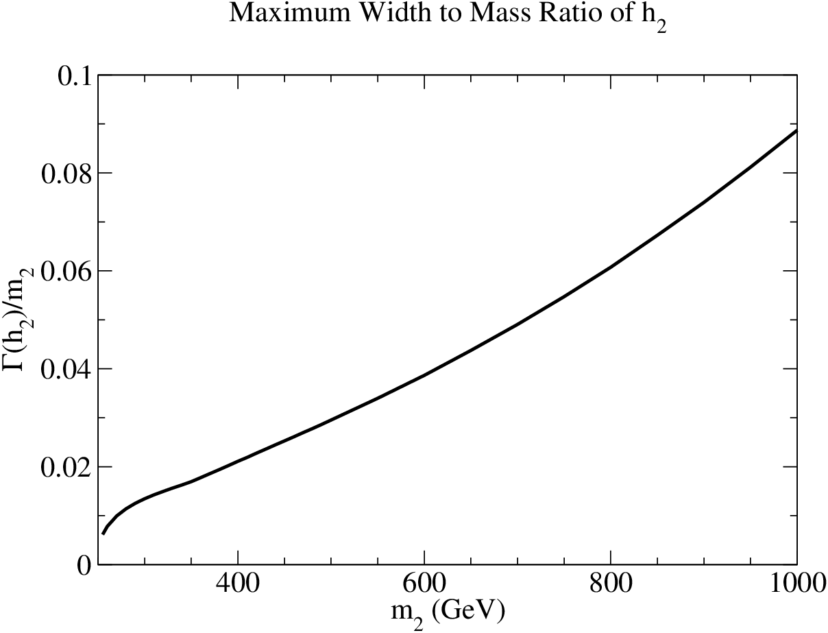
In Fig. 3 we show allowed ranges of $\Gamma(h_{2})/m_{2}$ as a function of the mass of $m_{2}$ for $b_{4}=4.2$ and $\sin^{2}\theta=0.12$. The total width is always bounded by $\Gamma(h_{2})/m_{2}\lesssim 0.09$. For $m_{2}\lesssim 700\textrm{ GeV}$, we also have $\Gamma(h_{2})/m_{2}\lesssim 0.05$. As $\sin\theta$ decreases below its upper bound, the total width of $h_{2}$ will decrease as well. The value of $b_{4}$ has no effect on the partial widths of $h_{2}$ into SM fermions or gauge bosons. However, as $b_{4}$ decreases, the partial width of $\Gamma(h_{2}\rightarrow h_{1}h_{1})$ decreases as shown in Fig. 2. Hence, the upper bound on $\Gamma(h_{2})$ in Fig. 3 is the upper bound throughout the allowed parameter regions, and $h_{2}$ is sufficiently narrow to justify the narrow width approximation in Eq. (18).

We maximize the production rate in Eq. (18) by fixing $m_{2}$ and $\theta$, then scanning over the remaining parameters

For all numerical results, the SM production cross sections and widths for a Higgs boson in Eqs. (16), (17), (19), and (20) were obtained from Ref. [82].

The maximum and minimum ${\rm BR}(h_{2}\rightarrow h_{1}h_{1})$ for different values of $m_{2}$ are shown in Fig. 4. We set $b_{4}=4.2$ at the perturbative unitarity bound and $\sin^{2}\theta=0.12$ at the experimental bound [31]. The largest possible branching ratio occurs at around $280\textrm{ GeV}$ with $\textrm{BR}(h_{2}\rightarrow h_{1}h_{1})=0.76$. Even up to masses of $1000\textrm{ GeV}$ the branching ratio to double Higgs can be larger than $0.3$. Additionally, for $m_{2}\gtrsim 600$ GeV there is a minimum on ${\rm BR}(h_{2}\rightarrow h_{1}h_{1})$.

Figure 5 shows the dependence of the maximum branching ratio ${\rm BR}(h_{2}\rightarrow h_{1}h_{1})$ on the parameter $b_{4}$. As can be seen, if the parameter $b_{4}$ is less than the unitarity bound of $4.2$ then the largest possible branching ratio becomes smaller. This is due to the shrinking of the allowed range for the parameters $a_{2}$ and $b_{3}$, as shown in Fig. 2. Even for small values of $b_{4}$, the branching ratio can still be quite substantial.

The maximum possible value of $\sin^{2}{\theta}$ is expected to decrease as more data is taken at the LHC and the measurements of the observed Higgs couplings become more precise. Figure 5 shows the maximum possible ${\rm BR}(h_{2}\rightarrow h_{1}h_{1})$ for several values of $\sin^{2}{\theta}$. As can be seen, the branching ratio can be larger for smaller $\sin\theta$. Hence, maximization of ${\rm BR}(h_{2}\rightarrow h_{1}h_{1})$ occurs at small $\sin\theta$. However, double Higgs production is not maximized with this condition.

Now we turn our attention to maximizing the double Higgs production rate. Figure 6 shows the maximum $\sigma(pp\rightarrow h_{2})\textrm{BR}(h_{2}\rightarrow h_{1}h_{1})$ at an LHC energy of $\sqrt{S_{H}}=13\textrm{ TeV}$ for various (a) $b_{4}$ and (b) $\sin\theta$ values as a function of mass $m_{2}$. The values are scaled by the SM double Higgs production cross section at $13\textrm{ TeV}$ of $33.53^{+5.3\%}_{-6.8\%}\textrm{ fb}$ [82], calculated at NNLL matched to NNLO in QCD with NLO top quark mass dependence [83]. As mentioned earlier, the maximum rates occur when $b_{4}$ is at the unitarity bound $b_{4}=4.2$. For $\sin\theta$, although the maximum ${\rm BR}(h_{2}\rightarrow h_{1}h_{1})$ increases as $\sin\theta$ decreases, this increase is not enough to compensate for the $\sin^{2}\theta$ suppression of the production cross section $\sigma(pp\rightarrow h_{2})$ in Eq. (19). Hence, the maximum double Higgs production cross section occurs at the experimental bound $\sin^{2}\theta=0.12$. In the best case, the resonant double Higgs production is roughly 30 times the SM double Higgs cross section.

Finally, we provide our benchmark points in Tables 1 and 2. We provide the parameter points that maximize the $h_{1}h_{1}$ production in the singlet extended SM, as well as the corresponding ${\rm BR}(h_{2}\rightarrow h_{1}h_{1})$ and $h_{1}h_{1}$ production cross section at a lab frame energy of $\sqrt{S_{H}}=13$ TeV. As discussed before, the maximum ${\rm BR}(h_{2}\rightarrow h_{1}h_{1})$ occurs for $b_{4}=4.2$ at the unitarity bound. Hence, we fix $b_{4}=4.2$ for all benchmark points. Also, the maximum $h_{1}h_{1}$ production cross section occurs for $\sin^{2}\theta=0.12$ at the current limit [31]. Table 1 contains the benchmark points for $\sin^{2}\theta=0.12$. However, as mentioned earlier, as the LHC continues to gather data it is expected that the precision Higgs measurements will further limit $\sin\theta$. The uncertainties in Higgs coupling measurements are projected to be $\sim 5\%$ with $3000\textrm{ fb}^{-1}$ of integrated luminosity at the LHC [84]. This corresponds to a bound of $\sin^{2}\theta\lesssim 0.05$ due to the overall $\cos^{2}\theta$ suppression of the $h_{1}$ rate of production. Hence, we also provide benchmark points for $\sin^{2}\theta=0.05$ in Table 2.

The simplest possible extension of the SM is the addition of a real gauge singlet scalar. Although simple, this model is theoretically well-motivated and has interesting phenomenology. In particular, if the new scalar $h_{2}$ is sufficiently heavy $m_{2}\geq 2\,m_{1}$, this model can give rise to resonant double Higgs production at the LHC. We have investigated this signature. We determined benchmark parameter points that maximize the double Higgs production rate in this model at the $\sqrt{S_{H}}=13$ TeV LHC. These benchmark points are important for gauging when the ongoing experimental searches for resonant double Higgs production are probing interesting regions of parameter space of well-motivated models. We have found that ${\rm BR}(h_{2}\rightarrow h_{1}h_{1})$ as high as $0.76$ and $h_{1}h_{1}$ production rates up to 30 times the SM rate are still possible.

We thank S. Dawson for valuable discussions about double Higgs production in the singlet extended SM. This investigation was supported in part by the University of Kansas General Research Fund allocation 2302091.

*

References

- [1] CMS Collaboration, S. Chatrchyan et al., “Observation of a new boson at a mass of 125 GeV with the CMS experiment at the LHC,” Phys. Lett. B716 (2012) 30–61, arXiv:1207.7235 [hep-ex].
- [2] ATLAS Collaboration, G. Aad et al., “Observation of a new particle in the search for the Standard Model Higgs boson with the ATLAS detector at the LHC,” Phys. Lett. B716 (2012) 1–29, arXiv:1207.7214 [hep-ex].
- [3] ATLAS, CMS Collaboration, G. Aad et al., “Measurements of the Higgs boson production and decay rates and constraints on its couplings from a combined ATLAS and CMS analysis of the LHC pp collision data at and 8 TeV,” JHEP 08 (2016) 045, arXiv:1606.02266 [hep-ex].
- [4] T. Binoth and J. J. van der Bij, “Influence of strongly coupled, hidden scalars on Higgs signals,” Z. Phys. C75 (1997) 17–25, arXiv:hep-ph/9608245 [hep-ph].
- [5] H. Davoudiasl, R. Kitano, T. Li, and H. Murayama, “The New minimal standard model,” Phys. Lett. B609 (2005) 117–123, arXiv:hep-ph/0405097 [hep-ph].
- [6] R. M. Schabinger and J. D. Wells, “A Minimal spontaneously broken hidden sector and its impact on Higgs boson physics at the large hadron collider,” Phys. Rev. D72 (2005) 093007, arXiv:hep-ph/0509209 [hep-ph].
- [7] B. Patt and F. Wilczek, “Higgs-field portal into hidden sectors,” arXiv:hep-ph/0605188 [hep-ph].
- [8] M. Bowen, Y. Cui, and J. D. Wells, “Narrow trans-TeV Higgs bosons and decays: Two LHC search paths for a hidden sector Higgs boson,” JHEP 03 (2007) 036, arXiv:hep-ph/0701035 [hep-ph].
- [9] S. Bock, R. Lafaye, T. Plehn, M. Rauch, D. Zerwas, and P. M. Zerwas, “Measuring Hidden Higgs and Strongly-Interacting Higgs Scenarios,” Phys. Lett. B694 (2010) 44–53, arXiv:1007.2645 [hep-ph].
- [10] A. Djouadi, O. Lebedev, Y. Mambrini, and J. Quevillon, “Implications of LHC searches for Higgs–portal dark matter,” Phys. Lett. B709 (2012) 65–69, arXiv:1112.3299 [hep-ph].
- [11] C. Englert, T. Plehn, M. Rauch, D. Zerwas, and P. M. Zerwas, “LHC: Standard Higgs and Hidden Higgs,” Phys. Lett. B707 (2012) 512–516, arXiv:1112.3007 [hep-ph].
- [12] C. Englert, T. Plehn, D. Zerwas, and P. M. Zerwas, “Exploring the Higgs portal,” Phys. Lett. B703 (2011) 298–305, arXiv:1106.3097 [hep-ph].
- [13] T. Alanne, K. Tuominen, and V. Vaskonen, “Strong phase transition, dark matter and vacuum stability from simple hidden sectors,” Nucl. Phys. B889 (2014) 692–711, arXiv:1407.0688 [hep-ph].
- [14] S. W. Ham, Y. S. Jeong, and S. K. Oh, “Electroweak phase transition in an extension of the standard model with a real Higgs singlet,” J. Phys. G31 no. 8, (2005) 857–871, arXiv:hep-ph/0411352 [hep-ph].
- [15] S. Profumo, M. J. Ramsey-Musolf, and G. Shaughnessy, “Singlet Higgs phenomenology and the electroweak phase transition,” JHEP 08 (2007) 010, arXiv:0705.2425 [hep-ph].
- [16] A. Ashoorioon and T. Konstandin, “Strong electroweak phase transitions without collider traces,” JHEP 07 (2009) 086, arXiv:0904.0353 [hep-ph].
- [17] D. Bodeker and G. D. Moore, “Can electroweak bubble walls run away?,” JCAP 0905 (2009) 009, arXiv:0903.4099 [hep-ph].
- [18] J. R. Espinosa, T. Konstandin, and F. Riva, “Strong Electroweak Phase Transitions in the Standard Model with a Singlet,” Nucl. Phys. B854 (2012) 592–630, arXiv:1107.5441 [hep-ph].
- [19] J. M. No and M. Ramsey-Musolf, “Probing the Higgs Portal at the LHC Through Resonant di-Higgs Production,” Phys. Rev. D89 no. 9, (2014) 095031, arXiv:1310.6035 [hep-ph].
- [20] D. Curtin, P. Meade, and C.-T. Yu, “Testing Electroweak Baryogenesis with Future Colliders,” JHEP 11 (2014) 127, arXiv:1409.0005 [hep-ph].
- [21] S. Profumo, M. J. Ramsey-Musolf, C. L. Wainwright, and P. Winslow, “Singlet-catalyzed electroweak phase transitions and precision Higgs boson studies,” Phys. Rev. D91 no. 3, (2015) 035018, arXiv:1407.5342 [hep-ph].
- [22] F. P. Huang and C. S. Li, “Electroweak baryogenesis in the framework of the effective field theory,” Phys. Rev. D92 no. 7, (2015) 075014, arXiv:1507.08168 [hep-ph].
- [23] P. H. Damgaard, A. Haarr, D. O’Connell, and A. Tranberg, “Effective Field Theory and Electroweak Baryogenesis in the Singlet-Extended Standard Model,” JHEP 02 (2016) 107, arXiv:1512.01963 [hep-ph].
- [24] J. Kozaczuk, “Bubble Expansion and the Viability of Singlet-Driven Electroweak Baryogenesis,” JHEP 10 (2015) 135, arXiv:1506.04741 [hep-ph].
- [25] P. Huang, A. Joglekar, B. Li, and C. E. M. Wagner, “Probing the Electroweak Phase Transition at the LHC,” Phys. Rev. D93 no. 5, (2016) 055049, arXiv:1512.00068 [hep-ph].
- [26] M.-L. Xiao and J.-H. Yu, “Electroweak baryogenesis in a scalar-assisted vectorlike fermion model,” Phys. Rev. D94 no. 1, (2016) 015011, arXiv:1509.02931 [hep-ph].
- [27] P. Huang, A. J. Long, and L.-T. Wang, “Probing the Electroweak Phase Transition with Higgs Factories and Gravitational Waves,” Phys. Rev. D94 no. 7, (2016) 075008, arXiv:1608.06619 [hep-ph].
- [28] A. V. Kotwal, M. J. Ramsey-Musolf, J. M. No, and P. Winslow, “Singlet-catalyzed electroweak phase transitions in the 100 TeV frontier,” Phys. Rev. D94 no. 3, (2016) 035022, arXiv:1605.06123 [hep-ph].
- [29] D. Curtin, P. Meade, and H. Ramani, “Thermal Resummation and Phase Transitions,” arXiv:1612.00466 [hep-ph].
- [30] V. Vaskonen, “Electroweak baryogenesis and gravitational waves from a real scalar singlet,” Phys. Rev. D95 (2017) , arXiv:1611.02073 [hep-ph].
- [31] ATLAS Collaboration, G. Aad et al., “Constraints on new phenomena via Higgs boson couplings and invisible decays with the ATLAS detector,” JHEP 11 (2015) 206, arXiv:1509.00672 [hep-ex].
- [32] ATLAS Collaboration, G. Aad et al., “Search for a high-mass Higgs boson decaying to a boson pair in collisions at TeV with the ATLAS detector,” JHEP 01 (2016) 032, arXiv:1509.00389 [hep-ex].
- [33] CMS Collaboration, V. Khachatryan et al., “Search for a Higgs boson in the mass range from 145 to 1000 GeV decaying to a pair of W or Z bosons,” JHEP 10 (2015) 144, arXiv:1504.00936 [hep-ex].
- [34] ATLAS Collaboration, G. Aad et al., “Search for an additional, heavy Higgs boson in the decay channel at in collision data with the ATLAS detector,” Eur. Phys. J. C76 no. 1, (2016) 45, arXiv:1507.05930 [hep-ex].
- [35] ATLAS Collaboration, G. Aad et al., “Searches for Higgs boson pair production in the channels with the ATLAS detector,” Phys. Rev. D92 (2015) 092004, arXiv:1509.04670 [hep-ex].
- [36] CMS Collaboration, V. Khachatryan et al., “Search for resonant pair production of Higgs bosons decaying to two bottom quark–antiquark pairs in proton–proton collisions at 8 TeV,” Phys. Lett. B749 (2015) 560–582, arXiv:1503.04114 [hep-ex].
- [37] CMS Collaboration, V. Khachatryan et al., “Search for two Higgs bosons in final states containing two photons and two bottom quarks in proton-proton collisions at 8 TeV,” Phys. Rev. D94 no. 5, (2016) 052012, arXiv:1603.06896 [hep-ex].
- [38] CMS Collaboration, “Search for resonant Higgs boson pair production in the final state using 2016 data,” CMS-PAS-HIG-16-029.
- [39] CMS Collaboration, “Search for resonant pair production of Higgs bosons decaying to two bottom quark-antiquark pairs in proton-proton collisions at 13 TeV,” CMS-PAS-HIG-16-002.
- [40] ATLAS Collaboration, “Search for pair production of Higgs bosons in the final state using protonproton collisions at TeV with the ATLAS detector,” ATLAS-CONF-2016-049.
- [41] ATLAS Collaboration, “Search for Higgs boson pair production in the final state using pp collision data at TeV with the ATLAS detector,” ATLAS-CONF-2016-004.
- [42] CMS Collaboration, “Measurements of properties of the Higgs boson and search for an additional resonance in the four-lepton final state at sqrt(s) = 13 TeV,” CMS-PAS-HIG-16-033.
- [43] CMS Collaboration, “Search for high mass Higgs to WW with fully leptonic decays using 2015 data,” CMS-PAS-HIG-16-023.
- [44] ATLAS Collaboration, “Study of the Higgs boson properties and search for high-mass scalar resonances in the decay channel at = 13 TeV with the ATLAS detector,” ATLAS-CONF-2016-079.
- [45] ATLAS Collaboration, “Search for a high-mass Higgs boson decaying to a pair of bosons in collisions at =13 TeV with the ATLAS detector,” ATLAS-CONF-2016-074.
- [46] ATLAS Collaboration, M. Aaboud et al., “Searches for heavy diboson resonances in collisions at TeV with the ATLAS detector,” JHEP 09 (2016) 173, arXiv:1606.04833 [hep-ex].
- [47] CMS Collaboration, “Search for resonances in boosted semileptonic final states in pp collisions at ,” CMS-PAS-B2G-15-002.
- [48] CMS Collaboration, V. Khachatryan et al., “Search for resonant production in proton-proton collisions at 8 TeV,” Phys. Rev. D93 no. 1, (2016) 012001, arXiv:1506.03062 [hep-ex].
- [49] ATLAS Collaboration, G. Aad et al., “A search for resonances using lepton-plus-jets events in proton-proton collisions at TeV with the ATLAS detector,” JHEP 08 (2015) 148, arXiv:1505.07018 [hep-ex].
- [50] D. O’Connell, M. J. Ramsey-Musolf, and M. B. Wise, “Minimal Extension of the Standard Model Scalar Sector,” Phys. Rev. D75 (2007) 037701, arXiv:hep-ph/0611014 [hep-ph].
- [51] V. Barger, P. Langacker, M. McCaskey, M. Ramsey-Musolf, and G. Shaughnessy, “Complex Singlet Extension of the Standard Model,” Phys. Rev. D79 (2009) 015018, arXiv:0811.0393 [hep-ph].
- [52] S. Dawson and W. Yan, “Hiding the Higgs Boson with Multiple Scalars,” Phys. Rev. D79 (2009) 095002, arXiv:0904.2005 [hep-ph].
- [53] D. Bertolini and M. McCullough, “The Social Higgs,” JHEP 12 (2012) 118, arXiv:1207.4209 [hep-ph].
- [54] G. M. Pruna and T. Robens, “Higgs singlet extension parameter space in the light of the LHC discovery,” Phys. Rev. D88 no. 11, (2013) 115012, arXiv:1303.1150 [hep-ph].
- [55] C. Caillol, B. Clerbaux, J.-M. Frère, and S. Mollet, “Precision versus discovery: A simple benchmark,” Eur. Phys. J. Plus 129 (2014) 93, arXiv:1304.0386 [hep-ph].
- [56] D. López-Val and T. Robens, “Δr and the W-boson mass in the singlet extension of the standard model,” Phys. Rev. D90 (2014) 114018, arXiv:1406.1043 [hep-ph].
- [57] D. Buttazzo, F. Sala, and A. Tesi, “Singlet-like Higgs bosons at present and future colliders,” JHEP 11 (2015) 158, arXiv:1505.05488 [hep-ph].
- [58] T. Robens and T. Stefaniak, “Status of the Higgs Singlet Extension of the Standard Model after LHC Run 1,” Eur. Phys. J. C75 (2015) 104, arXiv:1501.02234 [hep-ph].
- [59] A. Falkowski, C. Gross, and O. Lebedev, “A second Higgs from the Higgs portal,” JHEP 05 (2015) 057, arXiv:1502.01361 [hep-ph].
- [60] F. Bojarski, G. Chalons, D. Lopez-Val, and T. Robens, “Heavy to light Higgs boson decays at NLO in the Singlet Extension of the Standard Model,” JHEP 02 (2016) 147, arXiv:1511.08120 [hep-ph].
- [61] R. Costa, M. Mühlleitner, M. O. P. Sampaio, and R. Santos, “Singlet Extensions of the Standard Model at LHC Run 2: Benchmarks and Comparison with the NMSSM,” JHEP 06 (2016) 034, arXiv:1512.05355 [hep-ph].
- [62] O. Fischer, “Clues on the Majorana scale from scalar resonances at the LHC,” Mod. Phys. Lett. A32 no. 06, (2017) 1750035, arXiv:1607.00282 [hep-ph].
- [63] S. Fichet, G. von Gersdorff, E. Pontón, and R. Rosenfeld, “The Global Higgs as a Signal for Compositeness at the LHC,” JHEP 01 (2017) 012, arXiv:1608.01995 [hep-ph].
- [64] M. J. Dolan, C. Englert, and M. Spannowsky, “New Physics in LHC Higgs boson pair production,” Phys. Rev. D87 no. 5, (2013) 055002, arXiv:1210.8166 [hep-ph].
- [65] B. Cooper, N. Konstantinidis, L. Lambourne, and D. Wardrope, “Boosted : A new topology in searches for TeV-scale resonances at the LHC,” Phys. Rev. D88 no. 11, (2013) 114005, arXiv:1307.0407 [hep-ex].
- [66] C.-Y. Chen, S. Dawson, and I. M. Lewis, “Exploring resonant di-Higgs boson production in the Higgs singlet model,” Phys. Rev. D91 no. 3, (2015) 035015, arXiv:1410.5488 [hep-ph].
- [67] V. Martín Lozano, J. M. Moreno, and C. B. Park, “Resonant Higgs boson pair production in the decay channel,” JHEP 08 (2015) 004, arXiv:1501.03799 [hep-ph].
- [68] S. Dawson and I. M. Lewis, “NLO corrections to double Higgs boson production in the Higgs singlet model,” Phys. Rev. D92 no. 9, (2015) 094023, arXiv:1508.05397 [hep-ph].
- [69] S. I. Godunov, A. N. Rozanov, M. I. Vysotsky, and E. V. Zhemchugov, “Extending the Higgs sector: an extra singlet,” Eur. Phys. J. C76 (2016) 1, arXiv:1503.01618 [hep-ph].
- [70] T. Robens and T. Stefaniak, “LHC Benchmark Scenarios for the Real Higgs Singlet Extension of the Standard Model,” Eur. Phys. J. C76 no. 5, (2016) 268, arXiv:1601.07880 [hep-ph].
- [71] K. Nakamura, K. Nishiwaki, K.-y. Oda, S. C. Park, and Y. Yamamoto, “Di-higgs enhancement by neutral scalar as probe of new colored sector,” Eur. Phys. J. C77 no. 5, (2017) 273, arXiv:1701.06137 [hep-ph].
- [72] T. Huang, J. M. No, L. Pernié, M. Ramsey-Musolf, A. Safonov, M. Spannowsky, and P. Winslow, “Resonant Di-Higgs Production in the Channel: Probing the Electroweak Phase Transition at the LHC,” arXiv:1701.04442 [hep-ph].
- [73] J. Chang, C.-R. Chen, and C.-W. Chiang, “Higgs boson pair productions in the Georgi-Machacek model at the LHC,” JHEP 03 (2017) 137, arXiv:1701.06291 [hep-ph].
- [74] L.-C. Lü, C. Du, Y. Fang, H.-J. He, and H. Zhang, “Searching for Heavier Higgs Boson via Di-Higgs Production at LHC Run-2,” Phys. Lett. B755 (2016) 509–522, arXiv:1507.02644 [hep-ph].
- [75] J. Ren, R.-Q. Xiao, M. Zhou, Y. Fang, H.-J. He, and W. Yao, “LHC Search of New Higgs Boson via Resonant Di-Higgs Production with Decays into 4W,” arXiv:1706.05980 [hep-ph].
- [76] A. Schuessler and D. Zeppenfeld, “Unitarity constraints on MSSM trilinear couplings,” in SUSY 2007 Proceedings, 15th International Conference on Supersymmetry and Unification of Fundamental Interactions, July 26 - August 1, 2007, Karlsruhe, Germany, pp. 236–239. 2007. arXiv:0710.5175 [hep-ph].
- [77] P. Bechtle, O. Brein, S. Heinemeyer, G. Weiglein, and K. E. Williams, “HiggsBounds: Confronting Arbitrary Higgs Sectors with Exclusion Bounds from LEP and the Tevatron,” Comput. Phys. Commun. 181 (2010) 138–167, arXiv:0811.4169 [hep-ph].
- [78] P. Bechtle, O. Brein, S. Heinemeyer, G. Weiglein, and K. E. Williams, “HiggsBounds 2.0.0: Confronting Neutral and Charged Higgs Sector Predictions with Exclusion Bounds from LEP and the Tevatron,” Comput. Phys. Commun. 182 (2011) 2605–2631, arXiv:1102.1898 [hep-ph].
- [79] P. Bechtle et al., “Recent Developments in HiggsBounds and a Preview of HiggsSignals,” PoS CHARGED2012 (2012) 024, arXiv:1301.2345 [hep-ph].
- [80] P. Bechtle et al., “HiggsBounds-4: Improved Tests of Extended Higgs Sectors against Exclusion Bounds from LEP, the Tevatron and the LHC,” Eur. Phys. J. C74 (2014) 2693, arXiv:1311.0055 [hep-ph].
- [81] P. Bechtle, S. Heinemeyer, O. Stal, T. Stefaniak, and G. Weiglein, “Applying Exclusion Likelihoods from LHC Searches to Extended Higgs Sectors,” Eur. Phys. J. C75 no. 9, (2015) 421, arXiv:1507.06706 [hep-ph].
- [82] LHC Higgs Cross Section Working Group Collaboration, D. de Florian et al., “Handbook of LHC Higgs Cross Sections: 4. Deciphering the Nature of the Higgs Sector,” arXiv:1610.07922 [hep-ph].
- [83] S. Borowka, N. Greiner, G. Heinrich, S. P. Jones, M. Kerner, J. Schlenk, and T. Zirke, “Full top quark mass dependence in Higgs boson pair production at NLO,” JHEP 10 (2016) 107, arXiv:1608.04798 [hep-ph].
- [84] S. Dawson et al., “Working Group Report: Higgs Boson,” in Proceedings, 2013 Community Summer Study on the Future of U.S. Particle Physics: Snowmass on the Mississippi (CSS2013): Minneapolis, MN, USA, July 29-August 6, 2013. 2013. arXiv:1310.8361 [hep-ex]. http://inspirehep.net/record/1262795/files/arXiv:1310.8361.pdf.