MSCM-LiFe: Multi-scale cross modal linear feature for horizon detection in maritime images
Abstract
This paper proposes a new method for horizon detection called the multi-scale cross modal linear feature. This method integrates three different concepts related to the presence of horizon in maritime images to increase the accuracy of horizon detection. Specifically it uses the persistence of horizon in multi-scale median filtering, and its detection as a linear feature commonly detected by two different methods, namely the Hough transform of edgemap and the intensity gradient. We demonstrate the performance of the method over 13 videos comprising of more than 3000 frames and show that the proposed method detects horizon with small error in most of the cases, outperforming three state-of-the-art methods.
I Introduction
Horizon detection is useful in maritime electro optical data processing for various purposes [1], including registration for mobile sensor platforms such as buoys, maritime vessels, unmanned aerial vehicles [2, 3] and restricting the object search region [4, 5, 6]. In maritime scenario, horizon often appears as a linear feature and thus expected to be simple. However, several challenges may be encountered. An obvious challenge is the presence of the linear features of landmass, water-borne vessels, and air-borne objects. The other challenges encountered in visible range and near infrared sensors is the water patterns. Another challenge in data acquired from far infrared sensors is the continuous variation of intensity perpendicular to the horizon, which does not exhibit a sharp edge-like behaviour.
Conventional horizon detection methods use linear feature detectors such as Hough or Radon transform [4, 7, 8, 9, 10, 11, 12], statistical distributions representing the colors or intensity of the two regions created by a candidate horizon [13, 14, 15, 16, 17], classification of pixels as belonging to sea and sky [18, 19, 13], trends of change of intensity close to the horizon [20, 21], and the use of statistical features [22, 15, 16, 19]. We note that more than one concepts have been used before. For example, Hough transform and distances between statistical distributions have been used in [14]. Multi-scale filtering has been used with intensity gradients in [20] and Radon transform in [23].
Linear feature detectors require that the line feature corresponding to horizon is represented by more number of edge pixels than any other line feature in the edge map. This requirement may not be met for horizon occluded by maritime objects or for presence of a long linear feature in image due to oceanic color differences, wakes, or long vessels in foreground [24]. Methods that use statistical distribution or statistical features are challenged by the color gamut of maritime videos which is largely the same in sky and sea regions but may have significant difference in the oceanic color due to depths and shadows. Methods that use trends of intensity change close to horizon are affected adversely by occlusion. A method that is robust to such scenarios is needed.
Here, we propose a new method called Multi-Scale Cross Modal Linear Feature (MSCM-LiFe). As the name implies, we use multi-scale approach. We additionally use two different modalities, Hough transform and intensity gradients, to find the line features which persist over these two modalities as well as over different scales. Thus, the method uses complementary as well as supplementary aspects of these approaches to provide better robustness to the above mentioned scenarios. The method is detailed in section II. Results and comparison with other methods are presented in III. The paper is concluded in section IV.
II Proposed method
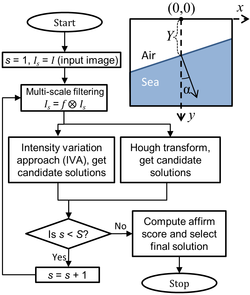
The flowchart of the proposed method is shown in Fig. 1. The horizon is represented using , the vertical distance of the horizon from the center point of upper edge of the image, and , the angle made by the normal to the horizon pointing into the sea with the axis shown in inset of Fig. 1. The details of the functional blocks, namely multi-scale filtering, Hough transform, intensity variation approach (IVA), and the computation of affirm score for selection of the final solution are presented below.
Multiscale filter — Here we explain the computation of multi-scale images and mean multi-scale images which are used in the Hough transform block and IVA block, respectively.
For the input image , we compute filtered image with vertical median filter of scale as follows:
| (1) |
Such multi-scale images are are computed for . The median filter smooths small random variations but retains the prominent edges, thus aiding the Hough transform. An example of the multi-scale images obtained from an image is given in Fig. 2.

Mean multi-scale image is also computed for each as follows:
| (2) |
The mean multi-scale image reinforces edges consistent over multiple scale, yet retains small details albeit with much smaller intensity. Bouma et. al reinforces used only the mean multi-scale image corresponding to the largest value of . But, we use mean multi-scale image corresponding to each value of in the IVA block.
Hough transform candidates — First, the binary edgemap of the multi-scale image is computed using canny edge detector. Then, Hough transform is applied on the edge map as follows:
| (3) |
The top 10 candidates with the largest values of are selected for each scale . Thus, a total of 100 candidates are collected using Hough transform. For each candidate , the parameters of the horizon and the Hough score is stored.
Intensity variation approach — For each vertical strip (i.e. a column of pixels in an image) characterized by pixel , the point is determined as follows:
| (4) |
This means that the point of maximum intensity variation is chosen for each strip of one pixel. Then, a line is fit on all these points. The line is used as a horizon candidate and corresponding to it is determined. For each scale , the candidate is determined. The mean value of the magnitude of intensity gradients for all the strips is used as the IVA score:
| (5) |
Affirm score and selection of final solution For each pair of Hough and IVA candidate , we compute two scores, a goodness score of the pair and the geometric proximity score of the pair. The goodness score quantifies the goodness of the pair in terms of the goodness of each candidate in the pair, i.e. goodness of the Hough transform for candidate and goodness of IVA for the candidate . The goodness score is defined as:
| (6) |
The geometric proximity score quantifies the geometric similarity of the candidates and in the candidate pair . It is defined as follows:
| (7) |
where is the number of pixels along the y-axis (i.e., the number of pixels in the frame along the vertical direction, see inset of 1), is the relative vertical distance between horizon candidates and ranges between . The normalization by is done because both Hough transform and IVA approaches gives candidates with the value of in the range . Consequently, represents the proximity of the candidates in terms of their vertical positions. The term represents the angular difference and lies in the range . However values close to , , and mean that the candidates have similar orientation. Thus, effectively represents proximity of the candidates in terms of orientation. Consequently, the geometric proximity score represents the proximity of the candidates in terms of both position and orientation.
Then, the affirm score is computed as the product of the goodness and geometric proximity scores:
| (8) |
The pair with the highest value of the affirm score is used to determine the final solution. The high value of the affirm score indicates the best cross-modal pair, in which the Hough candidate corresponds to a true line feature. On the contrary, IVA candidates is subject to line fitting errors due to fitting of line over points determined independently for each vertical strip. Thus, instead of using a combination of both the Hough and IVA candidates, only the Hough candidate is used as the final solution.
III Results and comparison
We present results of MSCM-LiFe and comparison with other methods in this section. We use 13 videos acquired using two Canon 70D cameras at 25 frames per second, one untouched camera for visible range videos, and another with hot mirror removed and NIR filter (BP800 Bandpass Filter by Midwest Optical Systems) added for near infrared videos. Among the visible range videos, 4 videos are taken on-board a ship while the other 5 videos are taken on-shore. Four NIR videos are taken in on-shore setup. Across these 13 videos, more that 3100 frames with various challenges are included. All frames are of high definition 1920 1080 pixels. Each frame in each video is annotated manually using a Matlab annotation tool and the annotation is used as the ground truth (GT). Across the frames, the GT values of range in and range in . I
| median() | median() (degrees) | ||||||||
| Video | Frames | MSCM-LiFe | ENIW [13] | FGSL [14] | MuSMF [20] | MSCM-LiFe | ENIW [13] | FGSL [14] | MuSMF [20] |
| Visible range on-board videos (camera is mounted on the ship and the ship is moving) | |||||||||
| V-1 | 299 | 5.7 | 37.8 | 37.5 | 170.2 | 0.6 | 0.5 | 0.5 | 0.5 |
| V-2 | 249 | 4.5 | 152.0 | 152.6 | 119.8 | 0.5 | 1.9 | 2.0 | 2.0 |
| V-3 | 249 | 3.2 | 174.8 | 17174.8 | 203.4 | 0.5 | 1.6 | 2.0 | 2.0 |
| V-4 | 249 | 6.5 | 69.5 | 69.8 | 331.2 | 0.7 | 1.2 | 1.3 | 1.3 |
| Visible range on-shore videos (camera is placed at shore on a fixed platform) | |||||||||
| V-5 | 110 | 8.9 | 130.3 | 130.3 | 90.6 | 0.3 | 11.2 | 11.1 | 10.7 |
| V-6 | 110 | 2.2 | 276.0 | 269.2 | 196.8 | 0.4 | 4.5 | 1.6 | 1.6 |
| V-7 | 299 | 9.7 | 34.6 | 34.6 | 145.5 | 0.7 | 0.8 | 0.7 | 0.7 |
| V-8 | 130 | 1.9 | 22.5 | 1.6 | 149.8 | 0.4 | 0.4 | 0.4 | 0.4 |
| V-9 | 299 | 3.0 | 24.8 | 2.8 | 103.2 | 0.4 | 1.3 | 0.4 | 0.4 |
| Near-infrared on-shore videos (camera is placed at shore on a fixed platform) | |||||||||
| V-10 | 83 | 1.9 | 720.5 | 651.1 | 507.7 | 1.0 | 1.5 | 0.9 | 0.9 |
| V-11 | 299 | 1.5 | 66.9 | 69.0 | 35.6 | 1.0 | 0.1 | 0.1 | 0.1 |
| V-12 | 299 | 1.2 | 5.4 | 5.2 | 60.9 | 0.2 | 1.0 | 0.4 | 0.4 |
| V-13 | 299 | 0.8 | 2.4 | 2.3 | 52.2 | 0.0 | 0.0 | 0.0 | 0.0 |
| Total | 3124 | 2.8 | 39.1 | 37.1 | 107.0 | 0.5 | 0.8 | 0.5 | 2.0 |
We compare the performance of the proposed method with 3 other methods (Author’s own Matlab implementations). For each method, the parameters and of the line detected as horizon are computed and compared with the ground truth. The methods used are the method of Ettinger et. al (ENIW) [13], method of Fefilatyev et. al (FGSL) [14], and multi-scale median filter based approach (MuSMF) [20]. These methods represent the state-of-the-art for horizon detection in maritime images. Further, Hough transform is used in FGSL and multi-scale IVA is used MuSMF. Thus, they can be considered predecessors of the proposed method.
 |
 |
| (a) Histogram of error in estimate of for all methods | (b) Histogram of error in estimate of for all methods |
 |
 |
| (c) Histogram zoom-in for MSCM-LiFe for | (d) Histogram zoom-in for MSCM-LiFe for |
The median of errors in the parameters for each of the videos are listed in Table I. It is seen that MSCM-LiFe performs consistently well giving a small median error for all of the videos. In comparison, all other methods perform poorer. The error is more accentuated in the parameter . Only for video V-13, the errors of 3 methods is parameter is less than 2.5 pixels.
We also plot the error histograms for both and parameters for all the frames in Fig. 3(a,b). While all algorithms have peak error values in the first bin, which is of the size 40 pixels for and 5∘ for , the proposed method have highest number of frames with peak error in the first bin which means lower error comparatively. A further zoom-in of the histograms for the proposed methods is shown in Fig. 3(c,d), which clearly indicates that the proposed method has very small error for most of the frames, within 10 pixels for the parameter for 80% of the frames and within 1∘ for the parameter for 86% of the frames. Some sample results are shown in Fig. 4.
The small percent of frames for which the MSCM-LiFe performs poor are typically the frames in which the foam of a long wake spanning the entire width of the frame causes very strong Hough candidates as well IVA candidates which are consistent across all the scales. Notably, all the methods fail in such scenario.

IV Conclusion
This paper has proposed multi-scale cross-modal line feature for horizon detection to overcome the challenges of horizon detection in images captured using electro-optical sensors. Usage of three concepts and two modalities ensures that the line feature persistent over multiple scales and occurring across more than one modality is chosen. The choice of such line feature is dictated by a newly proposed affirm score that checks the goodness of a line feature pair across the two modalities as well as the geometric proximity of the pair.
The method is tested for 13 videos comprising of more than 3000 frames, of which 4 videos were near-infrared and the others were visible range. The results show that the proposed method performs well even in the presence of severe occlusion, wakes, skyline, etc. It performs better than 3 contemporary methods which use concepts such as mutli-scale filtering, Hough transform, intensity variation, as well as statistical distances.
Acknowledgment
This work was conducted within Rolls Royce@NTU Corporate Lab with the support of National Research Foundation under the CorpLab@University scheme.
References
- [1] D. K. Prasad, D. Rajan, L. Rachmawati, E. Rajabally, and C. Quek, “Video processing from electro-optical sensors for object detection and tracking in maritime environment: A survey,” IEEE Transactions on Intelligent Transportation Systems, vol. 18, 2017.
- [2] S. Fefilatyev, D. Goldgof, and C. Lembke, “Tracking ships from fast moving camera through image registration,” in International Conference on Pattern Recognition, 2010, pp. 3500–3503.
- [3] X. Cao, Z. Rasheed, H. Liu, and N. Haering, “Automatic geo-registration of maritime video feeds,” in International Conference on Pattern Recognition, 2008, pp. 1–4.
- [4] D. Bloisi, L. Iocchi, M. Fiorini, and G. Graziano, “Automatic maritime surveillance with visual target detection,” in Proc. of the International Defense and Homeland Security Simulation Workshop, 2011, pp. 141–145.
- [5] S. P. van den Broek, H. Bouma, and M. A. Degache, “Discriminating small extended targets at sea from clutter and other classes of boats in infrared and visual light imagery,” in SPIE Defense and Security Symposium, 2008, pp. 69 690B–69 690B.
- [6] P. Voles, A. Smith, and M. K. Teal, “Nautical scene segmentation using variable size image windows and feature space reclustering,” in European Conference on Computer Vision. Springer, 2000, pp. 324–335.
- [7] D. Tang, G. Sun, D.-h. Wang, Z.-d. Niu, and Z.-p. Chen, “Research on infrared ship detection method in sea-sky background,” in International Symposium on Photoelectronic Detection and Imaging, 2013, pp. 89 072H–89 072H.
- [8] G.-Q. Bao, S.-S. Xiong, and Z.-Y. Zhou, “Vision-based horizon extraction for micro air vehicle flight control,” IEEE Transactions on Instrumentation and Measurement, vol. 54, no. 3, pp. 1067–1072, 2005.
- [9] H. Zhang, P. Yin, X. Zhang, and X. Shen, “A robust adaptive horizon recognizing algorithm based on projection,” Transactions of the Institute of Measurement and Control, 2010.
- [10] H. Wei, H. Nguyen, P. Ramu, C. Raju, X. Liu, and J. Yadegar, “Automated intelligent video surveillance system for ships,” in SPIE Defense, Security, and Sensing, 2009, pp. 73 061N–73 061N.
- [11] D. Dusha, W. Boles, and R. Walker, “Attitude estimation for a fixed-wing aircraft using horizon detection and optical flow,” in Digital Image Computing Techniques and Applications, 2007, pp. 485–492.
- [12] T. G. McGee, R. Sengupta, and K. Hedrick, “Obstacle detection for small autonomous aircraft using sky segmentation,” in International Conference on Robotics and Automation, 2005, pp. 4679–4684.
- [13] S. M. Ettinger, M. C. Nechyba, P. G. Ifju, and M. Waszak, “Vision-guided flight stability and control for micro air vehicles,” Advanced Robotics, vol. 17, no. 7, pp. 617–640, 2003.
- [14] S. Fefilatyev, D. Goldgof, M. Shreve, and C. Lembke, “Detection and tracking of ships in open sea with rapidly moving buoy-mounted camera system,” Ocean Engineering, vol. 54, pp. 1–12, 2012.
- [15] T. Y. van Valkenburg-van Haarst and K. A. Scholte, “Polynomial background estimation using visible light video streams for robust automatic detection in a maritime environment,” in SPIE Europe Security+ Defence, 2009, pp. 748 209–748 209.
- [16] C. Demonceaux, P. Vasseur, and C. Pégard, “Omnidirectional vision on UAV for attitude computation,” in IEEE International Conference on Robotics and Automation, 2006, pp. 2842–2847.
- [17] S. Todorovic and M. C. Nechyba, “A vision system for intelligent mission profiles of micro air vehicles,” IEEE Transactions on Vehicular Technology, vol. 53, no. 6, pp. 1713–1725, 2004.
- [18] ——, “A vision system for horizon tracking and object recognition for micro air vehicles,” in Proc. Florida Conference on Recent Advances in Robotics, 2004.
- [19] B. Bhanu and R. D. Holben, “Model-based segmentation of FLIR images,” IEEE Transactions on Aerospace and Electronic Systems, vol. 26, no. 1, pp. 2–11, 1990.
- [20] H. Bouma, D.-J. J. de Lange, S. P. van den Broek, R. A. Kemp, and P. B. Schwering, “Automatic detection of small surface targets with electro-optical sensors in a harbor environment,” in SPIE Europe Security and Defence, 2008, pp. 711 402–711 402.
- [21] E. Gershikov, T. Libe, and S. Kosolapov, “Horizon Line Detection in Marine Images: Which Method to Choose?” International Journal on Advances in Intelligent Systems, vol. 6, no. 1 & 2, 2013.
- [22] S. Fefilatyev, V. Smarodzinava, L. O. Hall, and D. B. Goldgof, “Horizon detection using machine learning techniques,” in International Conference on Machine Learning and Applications, 2006, pp. 17–21.
- [23] D. K. Prasad, D. Rajan, L. Rachmawati, E. Rajabaly, and C. Quek, “MuSCoWERT: multi-scale consistence of weighted edge radon transform for horizon detection in maritime images,” Journal of Optical Society of America A, vol. 33, no. 12, pp. 2491–2500, 2017.
- [24] D. K. Prasad, K. C. Prasath, D. Rajan, C. Quek, L. Rachmawati, and E. Rajabally, “Challenges in video based object detection in maritime scenario using computer vision,” in International Conference on Connected Vehicles, 2017.