An Efficient Algebraic Solution to the Perspective-Three-Point Problem

Tong Ke

Stergios Roumeliotis Address: University of Minnesota Address: Minneapolis, MN 55455 Email: kexxx069@cs.umn.edu Address: University of Minnesota Address: Minneapolis, MN 55455 Email: stergios@cs.umn.edu

Abstract

In this work, we present an algebraic solution to the classical perspective-3-point (P3P) problem for determining the position and attitude of a camera from observations of three known reference points. In contrast to previous approaches, we first directly determine the camera’s attitude by employing the corresponding geometric constraints to formulate a system of trigonometric equations. This is then efficiently solved, following an algebraic approach, to determine the unknown rotation matrix and subsequently the camera’s position. As compared to recent alternatives, our method avoids computing unnecessary (and potentially numerically unstable) intermediate results, and thus achieves higher numerical accuracy and robustness at a lower computational cost. These benefits are validated through extensive Monte-Carlo simulations for both nominal and close-to-singular geometric configurations.

1 Introduction

The Perspective-n-Point (PnP) is the problem of determining the 3D position and orientation (pose) of a camera from observations of known point features. The PnP is typically formulated and solved linearly by employing lifting (e.g., [1]), or as a nonlinear least-squares problem minimized iteratively (e.g., [10]) or directly (e.g., [12]). The minimal case of the PnP (for n=3) is often used in practice, in conjunction with RANSAC, for removing outliers [5].

The first solution to the P3P problem was given by Grunert [9] in 1841. Since then, several methods have been introduced, some of which [9, 4, 19, 5, 17, 8] were reviewed and compared, in terms of numerical accuracy, by Haralick et al. [11]. Common to these algorithms is that they employ the law of cosines to formulate a system of three quadratic equations in the features’ distances from the camera. They differ, however, in the elimination process followed for arriving at a univariate polynomial. Later on, Quan and Lan [21] and more recently Gao et al. [6] employed the same formulation but instead used the Sylvester resultant [3] and Wu-Ritz’s zero-decomposition method [23], respectively, to solve the resulting system of equations, and, in the case of [6], to determine the number of real solutions. Regardless of the approach followed, once the feature’s distances have been computed, finding the camera’s orientation, expressed as a unit quaternion [13] or a rotation matrix [14], often requires computing the eigenvectors of a $4\times 4$ matrix (e.g., [21]) or performing singular value decomposition (SVD) of a $3\times 3$ matrix (e.g., [6]), respectively, both of which are time-consuming. Furthermore, numerical error propagation from the computed distances to the rotation matrix significantly reduces the accuracy of the computed pose estimates.

To the best of our knowledge, the first method¹¹ 1 Nister and Stewenius [20] also follow a geometric approach for solving the generalized P3P resulting into an octic univariate polynomial whose odd monomials vanish for the case of the central P3P. that does not employ the law of cosines in its P3P problem formulation is that of Kneip et al. [15], and later on that of Masselli and Zell [18]. Specifically, [15] and [18] follow a geometric approach for avoiding computing the features’ distances and instead directly solve for the camera’s pose. In both cases, however, several intermediate terms (e.g., tangents and cotangents of certain angles) need to be computed, which negatively affect the speed and numerical precision of the resulting algorithms.

Similar to [15] and [18], our proposed approach does not require first computing the features’ distances. Differently though, in our derivation, we first eliminate the camera’s position and the features’ distances to result into a system of three equations involving only the camera’s orientation. Then, we follow an algebraic process for successively eliminating two of the unknown 3-dof and arriving into a quartic polynomial. Our algorithm (summarized in Alg. 1) requires fewer operations and involves simpler and numerically more stable expressions, as compared to either [15] or [18], and thus performs better in terms of efficiency, accuracy, and robustness. Specifically, the main advantages of our approach are:

•

Our algorithm’s implementation takes about 40% of the time required by the current state of the art [15]. ²² 2 Although Masselli and Zell [18] claim that their algorithm runs faster than Kneip et al.’s [15], our results (see Section 3) show the opposite to be true (by a small margin). The reason we arrive at a different conclusion is that our simulation randomly generates a new geometric configuration for each run, while Masselli employs only one configuration during their entire simulation, in which they save time due to caching.
•

Our method achieves better accuracy than [15, 18] under nominal conditions. Moreover, we are able to further improve the numerical precision by applying root polishing to the solutions of the quartic polynomial while remaining faster than [15, 18].
•

Our algorithm is more robust than [15, 18] when considering close-to-singular configurations (the three points are almost collinear or very close to each other).

The remaining of this paper is structured as follows. Section 2 presents the definition of the P3P problem, as well as our derivations for estimating first the orientation and then the position of the camera. In Section 3, we assess the performance of our approach against [15] and [18] in simulation for both nominal and singular configurations. Finally, we conclude our work in Section 4.

2 Problem Formulation and Solution

2.1 Problem Definition

Given the positions, ${}^{\scriptscriptstyle{G}}\mathbf{p}_{i}$ , of three known features $f_{i},\ i=1,2,3$ , with respect to a reference frame $\{G\}$ , and the corresponding unit-vector, bearing measurements, ${}^{\scriptscriptstyle{C}}\mathbf{b}_{i}$ , $i=1,2,3$ , our objective is to estimate the position, ${}^{\scriptscriptstyle{G}}\mathbf{p}_{\scriptscriptstyle{C}}$ , and orientation, i.e., the rotation matrix ${}^{\scriptscriptstyle{G}}_{\scriptscriptstyle{C}}\mathbf{C}$ , of the camera $\{C\}$ .

2.2 Solving for the orientation

From the geometry of the problem (see Fig. 1), we have (for $i=1,2,3$ ):

{}^{\scriptscriptstyle{G}}\mathbf{p}_{i}

\displaystyle={}^{\scriptscriptstyle{G}}\mathbf{p}_{\scriptscriptstyle{C}}+d_{i}{}^{\scriptscriptstyle{G}}_{\scriptscriptstyle{C}}\mathbf{C}{}^{\scriptscriptstyle{C}}\mathbf{b}_{i}

(1)

where $d_{i}\triangleq\|^{\scriptscriptstyle{G}}\mathbf{p}_{\scriptscriptstyle{C}}-{}^{\scriptscriptstyle{G}}\mathbf{p}_{i}\|$ is the distance between the camera and the feature $f_{i}$ .

Refer to caption — Figure 1: The camera $\{C\}$ , whose position, ${}^{\scriptscriptstyle{G}}\mathbf{p}_{\scriptscriptstyle{C}}$ , and orientation, ${}^{\scriptscriptstyle{G}}_{\scriptscriptstyle{C}}\mathbf{C}$ , we seek to determine, observes unit-vector bearing measurement ${}^{\scriptscriptstyle{C}}\mathbf{b}_{i}$ of a feature $f_{i}$ , whose position, ${}^{\scriptscriptstyle{G}}\mathbf{p}_{i}$ , is known.

In order to eliminate the unknown camera position, ${}^{\scriptscriptstyle{G}}\mathbf{p}_{\scriptscriptstyle{C}}$ , and feature distance, $d_{i},\ i=1,2,3$ , we subtract pairwise the three equations corresponding to (1) for $(i,j)=(1,2),\ (1,3)$ and $(2,3)$ , and project them on the vector ${}^{\scriptscriptstyle{G}}_{\scriptscriptstyle{C}}\mathbf{C}({}^{\scriptscriptstyle{C}}\mathbf{b}_{i}\times{}^{\scriptscriptstyle{C}}\mathbf{b}_{j})$ to yield the following system of 3 equations in the unknown rotation ${}^{\scriptscriptstyle{G}}_{\scriptscriptstyle{C}}\mathbf{C}$ :

$\displaystyle(^{\scriptscriptstyle{G}}\mathbf{p}_{1}-{}^{\scriptscriptstyle{G}}\mathbf{p}_{2})^{\scriptscriptstyle{T}}{}^{\scriptscriptstyle{G}}_{\scriptscriptstyle{C}}\mathbf{C}({}^{\scriptscriptstyle{C}}\mathbf{b}_{1}\times{}^{\scriptscriptstyle{C}}\mathbf{b}_{2})$	$\displaystyle=0$	(2)
$\displaystyle(^{\scriptscriptstyle{G}}\mathbf{p}_{1}-{}^{\scriptscriptstyle{G}}\mathbf{p}_{3})^{\scriptscriptstyle{T}}{}^{\scriptscriptstyle{G}}_{\scriptscriptstyle{C}}\mathbf{C}({}^{\scriptscriptstyle{C}}\mathbf{b}_{1}\times{}^{\scriptscriptstyle{C}}\mathbf{b}_{3})$	$\displaystyle=0$	(3)
$\displaystyle(^{\scriptscriptstyle{G}}\mathbf{p}_{2}-{}^{\scriptscriptstyle{G}}\mathbf{p}_{3})^{\scriptscriptstyle{T}}{}^{\scriptscriptstyle{G}}_{\scriptscriptstyle{C}}\mathbf{C}({}^{\scriptscriptstyle{C}}\mathbf{b}_{2}\times{}^{\scriptscriptstyle{C}}\mathbf{b}_{3})$	$\displaystyle=0$	(4)

Next, and in order to compute one of the 3 unknown degrees of rotational freedom, we introduce the following factorization of ${}^{\scriptscriptstyle{G}}_{\scriptscriptstyle{C}}\mathbf{C}$ :

{}^{\scriptscriptstyle{G}}_{\scriptscriptstyle{C}}\mathbf{C}=\mathbf{C}(\mathbf{k}_{1},\theta_{1})\mathbf{C}(\mathbf{k}_{2},\theta_{2})\mathbf{C}(\mathbf{k}_{3},\theta_{3})

(5)

where³³ 3 $\mathbf{C}(\mathbf{k},\theta)$ denotes the rotation matrix describing the rotation about the unit vector, $\mathbf{k}$ , by an angle $\theta$ . Note that in the ensuing derivations, all rotation angles are defined using the left-hand rule.

\displaystyle\mathbf{k}_{1}\triangleq\frac{{}^{\scriptscriptstyle{G}}\mathbf{p}_{1}-{}^{\scriptscriptstyle{G}}\mathbf{p}_{2}}{\|{}^{\scriptscriptstyle{G}}\mathbf{p}_{1}-{}^{\scriptscriptstyle{G}}\mathbf{p}_{2}\|},\ \mathbf{k}_{3}\triangleq\frac{{}^{\scriptscriptstyle{C}}\mathbf{b}_{1}\times{}^{\scriptscriptstyle{C}}\mathbf{b}_{2}}{\|{}^{\scriptscriptstyle{C}}\mathbf{b}_{1}\times{}^{\scriptscriptstyle{C}}\mathbf{b}_{2}\|},\ \mathbf{k}_{2}\triangleq\frac{\mathbf{k}_{1}\times\mathbf{k}_{3}}{\|\mathbf{k}_{1}\times\mathbf{k}_{3}\|}

(6)

Substituting (5) in (2), yields a scalar equation in the unknown $\theta_{2}$ :

\displaystyle\mathbf{k}_{1}^{\scriptscriptstyle{T}}\mathbf{C}(\mathbf{k}_{2},\theta_{2})\mathbf{k}_{3}

\displaystyle=0

(7)

which we solve by employing Rodrigues’ rotation formula [16]:⁴⁴ 4 $\lfloor\mathbf{k}\rfloor$ denotes the $3\times 3$ skew-symmetric matrix corresponding to $\mathbf{k}$ such that $\lfloor\mathbf{k}\rfloor\mathbf{a}=\mathbf{k}\times\mathbf{a}$ , $\forall\ \mathbf{k},\mathbf{a}\in\mathbb{R}^{3}$ . Note also that if $\mathbf{k}$ is a unit vector, then $\lfloor\mathbf{k}\rfloor^{2}=\mathbf{k}\mathbf{k}^{\scriptscriptstyle{T}}-\mathbf{I}$ , while for two vectors $\mathbf{a}$ , $\mathbf{b}$ , $\lfloor\mathbf{a}\rfloor\lfloor\mathbf{b}\rfloor=\mathbf{b}\mathbf{a}^{\scriptscriptstyle{T}}-(\mathbf{a}^{\scriptscriptstyle{T}}\mathbf{b})\mathbf{I}$ . Lastly, it is easy to show that $\lfloor\lfloor\mathbf{a}\rfloor\mathbf{b}\rfloor=\mathbf{b}\mathbf{a}^{\scriptscriptstyle{T}}-\mathbf{a}\mathbf{b}^{\scriptscriptstyle{T}}.$

\mathbf{C}(\mathbf{k}_{2},\theta_{2})=\cos\theta_{2}\mathbf{I}-\sin\theta_{2}\lfloor\mathbf{k}_{2}\rfloor+(1-\cos\theta_{2})\mathbf{k}_{2}\mathbf{k}_{2}^{\scriptscriptstyle{T}}

(8)

to get

\displaystyle\theta_{2}=\arccos(\mathbf{k}_{1}^{\scriptscriptstyle{T}}\mathbf{k}_{3})\pm\frac{\pi}{2}

(9)

Note that we only need to consider one of these two solutions [in our case, we select $\theta_{2}=\arccos(\mathbf{k}_{1}^{\scriptscriptstyle{T}}\mathbf{k}_{3})-\frac{\pi}{2}$ ; see Fig. 2], since the other one will result in the same ${}^{\scriptscriptstyle{G}}_{\scriptscriptstyle{C}}\mathbf{C}$ (see Appendix 5.2 for a formal proof).
In what follows, we describe the process for eliminating $\theta_{3}$ from (3) and (4), and eventually arriving into a quartic polynomial involving a trigonometric function of $\theta_{1}$ . To do so, we once again substitute in (3) and (4) the factorization of ${}^{\scriptscriptstyle{G}}_{\scriptscriptstyle{C}}\mathbf{C}$ defined in (5) to get (for $i=1,2$ ):

\mathbf{u}_{i}^{\scriptscriptstyle{T}}\mathbf{C}(\mathbf{k}_{1},\theta_{1})\mathbf{C}(\mathbf{k}_{2},\theta_{2})\mathbf{C}(\mathbf{k}_{3},\theta_{3})\mathbf{v}_{i}=0

(10)

where

\displaystyle\mathbf{u}_{i}\triangleq{}^{\scriptscriptstyle{G}}\mathbf{p}_{i}-{}^{\scriptscriptstyle{G}}\mathbf{p}_{3},~~\mathbf{v}_{i}

\displaystyle\triangleq{}^{\scriptscriptstyle{C}}\mathbf{b}_{i}\times{}^{\scriptscriptstyle{C}}\mathbf{b}_{3},~~i=1,2,

(11)

and employ the following property of rotation matrices

\mathbf{C}(\mathbf{k}_{1},\theta_{1})\mathbf{C}(\mathbf{k}_{2},\theta_{2})\mathbf{C}^{\scriptscriptstyle{T}}(\mathbf{k}_{1},\theta_{1})=\mathbf{C}(\mathbf{C}(\mathbf{k}_{1},\theta_{1})\mathbf{k}_{2},\theta_{2})

to rewrite (10) in a simpler form as

	$\displaystyle\mathbf{u}_{i}^{\scriptscriptstyle{T}}\mathbf{C}(\mathbf{k}_{1},\theta_{1})\mathbf{C}(\mathbf{C}(\mathbf{k}_{2},\theta_{2})\mathbf{k}_{3},\theta_{3})\mathbf{C}(\mathbf{k}_{2},\theta_{2})\mathbf{v}_{i}$	$\displaystyle=0$
	$\displaystyle\Rightarrow\mathbf{u}_{i}^{\scriptscriptstyle{T}}\mathbf{C}(\mathbf{k}_{1},\theta_{1})\mathbf{C}(\mathbf{k}^{\prime}_{3},\theta_{3})\mathbf{v}^{\prime}_{i}$	$\displaystyle=0$		(12)

where

	$\displaystyle\mathbf{v}^{\prime}_{i}$	$\displaystyle\triangleq\mathbf{C}(\mathbf{k}_{2},\theta_{2})\mathbf{v}_{i},\ i=1,2$
	$\displaystyle\mathbf{k}^{\prime}_{3}$	$\displaystyle\triangleq\mathbf{C}(\mathbf{k}_{2},\theta_{2})\mathbf{k}_{3}=\mathbf{k}_{2}\times\mathbf{k}_{1}$		(13)

The last equality in (13) is geometrically depicted in Fig. 2 and algebraically derived in Appendix 5.1. Analogously, it is straightforward to show that

\mathbf{k}^{\prime}_{1}\triangleq\mathbf{C}^{\scriptscriptstyle{T}}(\mathbf{k}_{2},\theta_{2})\mathbf{k}_{1}=\mathbf{k}_{3}\times\mathbf{k}_{2}

Figure 2: Geometric relation between unit vectors

\mathbf{k}_{1},\ \mathbf{k}_{2},\ \mathbf{k}_{3},\ \mathbf{k}_{3}^{\prime},\ \mathbf{k}_{3}^{\prime\prime},

and

\mathbf{u}_{1}

. Note that

\mathbf{k}_{1},\ \mathbf{k}_{3}

, and

\mathbf{k}_{3}^{\prime}

belong to a plane

\pi_{1}

whose normal is

\mathbf{k}_{2}

. Also,

\mathbf{k}_{2},\ \mathbf{k}_{3}^{\prime}

, and

\mathbf{k}_{3}^{\prime\prime}

lie on a plane,

\pi_{2}

, normal to

\pi_{1}

Next, by employing Rodrigues’ rotation formula [see (8)], for expressing the product of a rotation matrix and a vector as a linear function of the unknown $\begin{bmatrix}\cos\theta&\sin\theta\end{bmatrix}^{\scriptscriptstyle{T}}$ , i.e.,

	$\displaystyle\mathbf{C}(\mathbf{k},\theta)\mathbf{v}$	$\displaystyle=(-\cos\theta\lfloor\mathbf{k}\rfloor^{2}-\sin\theta\lfloor\mathbf{k}\rfloor+\mathbf{k}\mathbf{k}^{\scriptscriptstyle{T}})\mathbf{v}$
		$\displaystyle=\begin{bmatrix}-\lfloor\mathbf{k}\rfloor^{2}\mathbf{v}&-\lfloor\mathbf{k}\rfloor\mathbf{v}\end{bmatrix}\begin{bmatrix}\cos\theta\\ \sin\theta\end{bmatrix}+(\mathbf{k}^{\scriptscriptstyle{T}}\mathbf{v})\mathbf{k}$		(14)

in (12) yields (for $i=1,2$ ):

		$\displaystyle\left(\begin{bmatrix}-\lfloor\mathbf{k}_{1}\rfloor^{2}\mathbf{u}_{i}&\lfloor\mathbf{k}_{1}\rfloor\mathbf{u}_{i}\end{bmatrix}\begin{bmatrix}\cos\theta_{1}\\ \sin\theta_{1}\end{bmatrix}+(\mathbf{k}_{1}^{\scriptscriptstyle{T}}\mathbf{u}_{i})\mathbf{k}_{1}\right)^{\scriptscriptstyle{T}}$
	$\displaystyle\cdot$	$\displaystyle\left(\begin{bmatrix}-\lfloor\mathbf{k}^{\prime}_{3}\rfloor^{2}\mathbf{v}^{\prime}_{i}&-\lfloor\mathbf{k}^{\prime}_{3}\rfloor\mathbf{v}^{\prime}_{i}\end{bmatrix}\begin{bmatrix}\cos\theta_{3}\\ \sin\theta_{3}\end{bmatrix}+({\mathbf{k}^{\prime}_{3}}^{\scriptscriptstyle{T}}\mathbf{v}^{\prime}_{i})\mathbf{k}^{\prime}_{3}\right)=0$		(15)

Expanding (15) and rearranging terms, yields (for $i=1,2$ )

	$\displaystyle\begin{bmatrix}\cos\theta_{1}\\ \sin\theta_{1}\end{bmatrix}^{\scriptscriptstyle{T}}\begin{bmatrix}\mathbf{u}_{i}^{\scriptscriptstyle{T}}\lfloor\mathbf{k}_{1}\rfloor^{2}\lfloor\mathbf{k}^{\prime}_{3}\rfloor^{2}\mathbf{v}^{\prime}_{i}&\mathbf{u}_{i}^{\scriptscriptstyle{T}}\lfloor\mathbf{k}_{1}\rfloor^{2}\lfloor\mathbf{k}^{\prime}_{3}\rfloor\mathbf{v}^{\prime}_{i}\\ \mathbf{u}_{i}^{\scriptscriptstyle{T}}\lfloor\mathbf{k}_{1}\rfloor\lfloor\mathbf{k}^{\prime}_{3}\rfloor^{2}\mathbf{v}^{\prime}_{i}&\mathbf{u}_{i}^{\scriptscriptstyle{T}}\lfloor\mathbf{k}_{1}\rfloor\lfloor\mathbf{k}^{\prime}_{3}\rfloor\mathbf{v}^{\prime}_{i}\end{bmatrix}\begin{bmatrix}\cos\theta_{3}\\ \sin\theta_{3}\end{bmatrix}$
$\displaystyle+$	$\displaystyle(\mathbf{k}_{1}^{\scriptscriptstyle{T}}\mathbf{u}_{i})\begin{bmatrix}-\mathbf{k}_{1}^{\scriptscriptstyle{T}}\lfloor\mathbf{k}^{\prime}_{3}\rfloor^{2}\mathbf{v}^{\prime}_{i}&-\mathbf{k}_{1}^{\scriptscriptstyle{T}}\lfloor\mathbf{k}^{\prime}_{3}\rfloor\mathbf{v}^{\prime}_{i}\end{bmatrix}\begin{bmatrix}\cos\theta_{3}\\ \sin\theta_{3}\end{bmatrix}$
$\displaystyle=$	$\displaystyle({\mathbf{k}^{\prime}_{3}}^{\scriptscriptstyle{T}}\mathbf{v}^{\prime}_{i})\begin{bmatrix}\mathbf{u}_{i}^{\scriptscriptstyle{T}}\lfloor\mathbf{k}_{1}\rfloor\lfloor\mathbf{k}^{\prime}_{3}\rfloor\mathbf{k}_{1}&\mathbf{u}_{i}^{\scriptscriptstyle{T}}\lfloor\mathbf{k}_{1}\rfloor\mathbf{k}^{\prime}_{3}\end{bmatrix}\begin{bmatrix}\cos\theta_{1}\\ \sin\theta_{1}\end{bmatrix}$	(16)

Notice that the term $\mathbf{u}_{i}^{\scriptscriptstyle{T}}\lfloor\mathbf{k}_{1}\rfloor\lfloor\mathbf{k}^{\prime}_{3}\rfloor$ appears three times in (16), and

$\displaystyle\mathbf{u}_{1}^{\scriptscriptstyle{T}}\lfloor\mathbf{k}_{1}\rfloor\lfloor\mathbf{k}^{\prime}_{3}\rfloor$	$\displaystyle=\mathbf{u}_{1}^{\scriptscriptstyle{T}}\mathbf{k}^{\prime}_{3}\mathbf{k}_{1}^{\scriptscriptstyle{T}}$
	$\displaystyle=({}^{\scriptscriptstyle{G}}\mathbf{p}_{1}-{}^{\scriptscriptstyle{G}}\mathbf{p}_{3})^{\scriptscriptstyle{T}}\lfloor\mathbf{k}_{1}\rfloor\lfloor\mathbf{k}^{\prime}_{3}\rfloor$
	$\displaystyle=({}^{\scriptscriptstyle{G}}\mathbf{p}_{1}-{}^{\scriptscriptstyle{G}}\mathbf{p}_{2}+{}^{\scriptscriptstyle{G}}\mathbf{p}_{2}-{}^{\scriptscriptstyle{G}}\mathbf{p}_{3})^{\scriptscriptstyle{T}}\lfloor\mathbf{k}_{1}\rfloor\lfloor\mathbf{k}^{\prime}_{3}\rfloor$
	$\displaystyle=({}^{\scriptscriptstyle{G}}\mathbf{p}_{2}-{}^{\scriptscriptstyle{G}}\mathbf{p}_{3})^{\scriptscriptstyle{T}}\lfloor\mathbf{k}_{1}\rfloor\lfloor\mathbf{k}^{\prime}_{3}\rfloor$
	$\displaystyle=\mathbf{u}_{2}^{\scriptscriptstyle{T}}\mathbf{k}^{\prime}_{3}\mathbf{k}_{1}^{\scriptscriptstyle{T}}=\mathbf{u}_{2}^{\scriptscriptstyle{T}}\lfloor\mathbf{k}_{1}\rfloor\lfloor\mathbf{k}^{\prime}_{3}\rfloor$	(17)

This motivates to rewrite (12) as (for $i=1,2$ ):

$\displaystyle 0$	$\displaystyle=\mathbf{u}_{i}^{\scriptscriptstyle{T}}\mathbf{C}(\mathbf{k}_{1},\theta_{1})\mathbf{C}(\mathbf{k}^{\prime}_{3},\theta_{3})\mathbf{v}^{\prime}_{i}$
	$\displaystyle=\mathbf{u}_{i}^{\scriptscriptstyle{T}}\mathbf{C}(\mathbf{k}_{1},\theta_{1})\mathbf{C}(\mathbf{k}_{1},-\phi)\mathbf{C}(\mathbf{k}_{1},\phi)\mathbf{C}(\mathbf{k}^{\prime}_{3},\theta_{3})\mathbf{v}^{\prime}_{i}$
	$\displaystyle=\mathbf{u}_{i}^{\scriptscriptstyle{T}}\mathbf{C}(\mathbf{k}_{1},\theta_{1}-\phi)\mathbf{C}(\mathbf{C}(\mathbf{k}_{1},\phi)\mathbf{k}^{\prime}_{3},\theta_{3})\mathbf{C}(\mathbf{k}_{1},\phi)\mathbf{v}^{\prime}_{i}$
	$\displaystyle=\mathbf{u}_{i}^{\scriptscriptstyle{T}}\mathbf{C}(\mathbf{k}_{1},\theta_{1}^{\prime})\mathbf{C}(\mathbf{k}^{\prime\prime}_{3},\theta_{3})\mathbf{v}^{\prime\prime}_{i}$	(18)

where

\displaystyle\theta_{1}^{\prime}\triangleq\theta_{1}-\phi,\ \mathbf{v}^{\prime\prime}_{i}\triangleq\mathbf{C}(\mathbf{k}_{1},\phi)\mathbf{v}^{\prime}_{i},\ \mathbf{k}^{\prime\prime}_{3}\triangleq\mathbf{C}(\mathbf{k}_{1},\phi)\mathbf{k}^{\prime}_{3}

(19)

To simplify the equation analogous to (16) that will result from (18) [instead of (16)], we seek to find a $\phi$ (not necessarily unique) such that $\mathbf{u}_{1}^{\scriptscriptstyle{T}}\mathbf{k}^{\prime\prime}_{3}=0$ , and hence, $\mathbf{u}_{i}^{\scriptscriptstyle{T}}\lfloor\mathbf{k}_{1}\rfloor\lfloor\mathbf{k}^{\prime\prime}_{3}\rfloor=0$ [see (17)], i.e.,

$\displaystyle 0$	$\displaystyle=\mathbf{u}_{1}^{\scriptscriptstyle{T}}\mathbf{k}^{\prime\prime}_{3}=\mathbf{u}_{1}^{\scriptscriptstyle{T}}\mathbf{C}(\mathbf{k}_{1},\phi)\mathbf{k}^{\prime}_{3}$	(20)
	$\displaystyle=\mathbf{u}_{1}^{\scriptscriptstyle{T}}(\cos\phi\mathbf{I}-\sin\phi\lfloor\mathbf{k}_{1}\rfloor+(1-\cos\phi)\mathbf{k}_{1}\mathbf{k}_{1}^{\scriptscriptstyle{T}})\mathbf{k}^{\prime}_{3}$
	$\displaystyle=\cos\phi\mathbf{u}_{1}^{\scriptscriptstyle{T}}\mathbf{k}^{\prime}_{3}-\sin\phi\mathbf{u}_{1}^{\scriptscriptstyle{T}}\lfloor\mathbf{k}_{1}\rfloor\mathbf{k}^{\prime}_{3}$
	$\displaystyle=\cos\phi\mathbf{u}_{1}^{\scriptscriptstyle{T}}\mathbf{k}^{\prime}_{3}-\sin\phi\mathbf{u}_{1}^{\scriptscriptstyle{T}}\mathbf{k}_{2}$

\displaystyle\Rightarrow\begin{bmatrix}\cos\phi&\sin\phi\end{bmatrix}

\displaystyle=\frac{1}{\delta}\begin{bmatrix}\mathbf{u}_{1}^{\scriptscriptstyle{T}}\mathbf{k}_{2}&\mathbf{u}_{1}^{\scriptscriptstyle{T}}\mathbf{k}^{\prime}_{3}\end{bmatrix}

(21)

where

\displaystyle\delta\triangleq\sqrt{(\mathbf{u}_{1}^{\scriptscriptstyle{T}}\mathbf{k}^{\prime}_{3})^{2}+(\mathbf{u}_{1}^{\scriptscriptstyle{T}}\mathbf{k}_{2})^{2}}=\|\mathbf{u}_{1}\times\mathbf{k}_{1}\|

(22)

and thus [from (19) using (8)]

$\displaystyle\mathbf{k}_{3}^{\prime\prime}$	$\displaystyle=\cos\phi\mathbf{k}^{\prime}_{3}-\sin\phi\lfloor\mathbf{k}_{1}\rfloor\mathbf{k}^{\prime}_{3}+(1-\cos\phi)\mathbf{k}_{1}\mathbf{k}_{1}^{\scriptscriptstyle{T}}\mathbf{k}^{\prime}_{3}$
	$\displaystyle=(\mathbf{k}^{\prime}_{3}\mathbf{k}_{2}^{\scriptscriptstyle{T}}\mathbf{u}_{1}-\mathbf{k}_{2}{\mathbf{k}_{3}^{\prime}}^{\scriptscriptstyle{T}}\mathbf{u}_{1})/\delta=\mathbf{u}_{1}\times(\mathbf{k}^{\prime}_{3}\times\mathbf{k}_{2})/\delta$
	$\displaystyle=\frac{\mathbf{u}_{1}\times\mathbf{k}_{1}}{\\|\mathbf{u}_{1}\times\mathbf{k}_{1}\\|}$	(23)

Now, we can expand (18) using (14) to get an equation analogous to (16):

		$\displaystyle\begin{bmatrix}\cos\theta_{1}^{\prime}\\ \sin\theta_{1}^{\prime}\end{bmatrix}^{\scriptscriptstyle{T}}\begin{bmatrix}\mathbf{u}_{i}^{\scriptscriptstyle{T}}\lfloor\mathbf{k}_{1}\rfloor^{2}\lfloor\mathbf{k}^{\prime\prime}_{3}\rfloor^{2}\mathbf{v}^{\prime\prime}_{i}&\mathbf{u}_{i}^{\scriptscriptstyle{T}}\lfloor\mathbf{k}_{1}\rfloor^{2}\lfloor\mathbf{k}^{\prime\prime}_{3}\rfloor\mathbf{v}^{\prime\prime}_{i}\\ \mathbf{u}_{i}^{\scriptscriptstyle{T}}\lfloor\mathbf{k}_{1}\rfloor\lfloor\mathbf{k}^{\prime\prime}_{3}\rfloor^{2}\mathbf{v}^{\prime\prime}_{i}&\mathbf{u}_{i}^{\scriptscriptstyle{T}}\lfloor\mathbf{k}_{1}\rfloor\lfloor\mathbf{k}^{\prime\prime}_{3}\rfloor\mathbf{v}^{\prime\prime}_{i}\end{bmatrix}\begin{bmatrix}\cos\theta_{3}\\ \sin\theta_{3}\end{bmatrix}$
		$\displaystyle+(\mathbf{k}_{1}^{\scriptscriptstyle{T}}\mathbf{u}_{i})\begin{bmatrix}-\mathbf{k}_{1}^{\scriptscriptstyle{T}}\lfloor\mathbf{k}^{\prime\prime}_{3}\rfloor^{2}\mathbf{v}^{\prime\prime}_{i}&-\mathbf{k}_{1}^{\scriptscriptstyle{T}}\lfloor\mathbf{k}^{\prime\prime}_{3}\rfloor\mathbf{v}^{\prime\prime}_{i}\end{bmatrix}\begin{bmatrix}\cos\theta_{3}\\ \sin\theta_{3}\end{bmatrix}=$
		$\displaystyle({\mathbf{k}^{\prime\prime}_{3}}^{\scriptscriptstyle{T}}\mathbf{v}^{\prime\prime}_{i})\begin{bmatrix}\mathbf{u}_{i}^{\scriptscriptstyle{T}}\lfloor\mathbf{k}_{1}\rfloor\lfloor\mathbf{k}^{\prime\prime}_{3}\rfloor\mathbf{k}_{1}&\mathbf{u}_{i}^{\scriptscriptstyle{T}}\lfloor\mathbf{k}_{1}\rfloor\mathbf{k}^{\prime\prime}_{3}\end{bmatrix}\begin{bmatrix}\cos\theta_{1}^{\prime}\\ \sin\theta_{1}^{\prime}\end{bmatrix}$		(24)

Substituting $\mathbf{u}_{i}^{\scriptscriptstyle{T}}\lfloor\mathbf{k}_{1}\rfloor\lfloor\mathbf{k}^{\prime\prime}_{3}\rfloor=0$ [see (17)] in (24) and renaming terms, yields (for $i=1,2$ ):

	$\displaystyle\begin{bmatrix}\cos\theta_{1}^{\prime}\\ \sin\theta_{1}^{\prime}\end{bmatrix}^{\scriptscriptstyle{T}}\begin{bmatrix}\bar{f}_{i1}&\bar{f}_{i2}\\ 0&0\end{bmatrix}\begin{bmatrix}\cos\theta_{3}\\ \sin\theta_{3}\end{bmatrix}+\begin{bmatrix}\bar{f}_{i4}&\bar{f}_{i5}\end{bmatrix}\begin{bmatrix}\cos\theta_{3}\\ \sin\theta_{3}\end{bmatrix}$
$\displaystyle=$	$\displaystyle\begin{bmatrix}0&\bar{f}_{i3}\end{bmatrix}\begin{bmatrix}\cos\theta_{1}^{\prime}\\ \sin\theta_{1}^{\prime}\end{bmatrix}$
$\displaystyle\Rightarrow$	$\displaystyle\begin{bmatrix}\bar{f}_{i1}\cos\theta_{1}^{\prime}+\bar{f}_{i4}&\bar{f}_{i2}\cos\theta_{1}^{\prime}+\bar{f}_{i5}\end{bmatrix}\begin{bmatrix}\cos\theta_{3}\\ \sin\theta_{3}\end{bmatrix}=\bar{f}_{i3}\sin\theta_{1}^{\prime}$	(25)

where⁵⁵ 5 The simplified expressions for the following terms, shown after the second equality, require lengthy algebraic derivations which we omit due to space limitations.

	$\displaystyle\bar{f}_{i1}$	$\displaystyle\triangleq\mathbf{u}_{i}^{\scriptscriptstyle{T}}\lfloor\mathbf{k}_{1}\rfloor^{2}\lfloor\mathbf{k}^{\prime\prime}_{3}\rfloor^{2}\mathbf{v}^{\prime\prime}_{i}=\delta\mathbf{v}_{i}^{\scriptscriptstyle{T}}\mathbf{k}_{2}$
	$\displaystyle\bar{f}_{i2}$	$\displaystyle\triangleq\mathbf{u}_{i}^{\scriptscriptstyle{T}}\lfloor\mathbf{k}_{1}\rfloor^{2}\lfloor\mathbf{k}^{\prime\prime}_{3}\rfloor\mathbf{v}^{\prime\prime}_{i}=\delta\mathbf{v}_{i}^{\scriptscriptstyle{T}}\mathbf{k}_{1}^{\prime}$
	$\displaystyle\bar{f}_{i3}$	$\displaystyle\triangleq({\mathbf{k}^{\prime\prime}_{3}}^{\scriptscriptstyle{T}}\mathbf{v}^{\prime\prime}_{i})\mathbf{u}_{i}^{\scriptscriptstyle{T}}\lfloor\mathbf{k}_{1}\rfloor\mathbf{k}^{\prime\prime}_{3}=\delta\mathbf{v}_{i}^{\scriptscriptstyle{T}}\mathbf{k}_{3}$
	$\displaystyle\bar{f}_{i4}$	$\displaystyle\triangleq-(\mathbf{u}_{i}^{\scriptscriptstyle{T}}\mathbf{k}_{1})\mathbf{k}_{1}^{\scriptscriptstyle{T}}\lfloor\mathbf{k}^{\prime\prime}_{3}\rfloor^{2}\mathbf{v}^{\prime\prime}_{i}=(\mathbf{u}_{i}^{\scriptscriptstyle{T}}\mathbf{k}_{1})(\mathbf{v}_{i}^{\scriptscriptstyle{T}}\mathbf{k}_{1}^{\prime})$
	$\displaystyle\bar{f}_{i5}$	$\displaystyle\triangleq-(\mathbf{u}_{i}^{\scriptscriptstyle{T}}\mathbf{k}_{1})\mathbf{k}_{1}^{\scriptscriptstyle{T}}\lfloor\mathbf{k}^{\prime\prime}_{3}\rfloor\mathbf{v}^{\prime\prime}_{i}=-(\mathbf{u}_{i}^{\scriptscriptstyle{T}}\mathbf{k}_{1})(\mathbf{v}_{i}^{\scriptscriptstyle{T}}\mathbf{k}_{2})$

For $i=1,2$ , (25) results into the following system:

\begin{bmatrix}\bar{f}_{11}\cos\theta_{1}^{\prime}+\bar{f}_{14}&\bar{f}_{12}\cos\theta_{1}^{\prime}+\bar{f}_{15}\\ \bar{f}_{21}\cos\theta_{1}^{\prime}+\bar{f}_{24}&\bar{f}_{22}\cos\theta_{1}^{\prime}+\bar{f}_{25}\end{bmatrix}\begin{bmatrix}\cos\theta_{3}\\ \sin\theta_{3}\end{bmatrix}=\begin{bmatrix}\bar{f}_{13}\\ \bar{f}_{23}\end{bmatrix}\sin\theta_{1}^{\prime}

(26)

Note that since $\bar{f}_{11}\bar{f}_{14}+\bar{f}_{12}\bar{f}_{15}=0$ , we can further simplify (26) by introducing $\theta_{3}^{\prime}$ , where

\displaystyle\begin{bmatrix}\cos\theta_{3}^{\prime}\\ \sin\theta_{3}^{\prime}\end{bmatrix}\triangleq\begin{bmatrix}\frac{\bar{f}_{11}\cos\theta_{3}+\bar{f}_{12}\sin\theta_{3}}{\sqrt{\bar{f}_{11}^{2}+\bar{f}_{12}^{2}}}&-\frac{\bar{f}_{14}\cos\theta_{3}+\bar{f}_{15}\sin\theta_{3}}{\sqrt{\bar{f}_{14}^{2}+\bar{f}_{15}^{2}}}\end{bmatrix}^{\scriptscriptstyle{T}}

(27)

Replacing $\theta_{3}$ by $\theta_{3}^{\prime}$ in (26), we have

\begin{bmatrix}f_{11}\cos\theta_{1}^{\prime}&f_{15}\\ f_{21}\cos\theta_{1}^{\prime}+f_{24}&f_{22}\cos\theta_{1}^{\prime}+f_{25}\end{bmatrix}\begin{bmatrix}\cos\theta_{3}^{\prime}\\ \sin\theta_{3}^{\prime}\end{bmatrix}=\begin{bmatrix}f_{13}\\ f_{23}\end{bmatrix}\sin\theta_{1}^{\prime}

(28)

where

$\displaystyle f_{11}$	$\displaystyle\triangleq\delta\mathbf{k}_{3}^{\scriptscriptstyle{T}}{}^{\scriptscriptstyle{C}}\mathbf{b}_{3}$	(29)
$\displaystyle f_{21}$	$\displaystyle\triangleq\delta({}^{\scriptscriptstyle{C}}\mathbf{b}_{1}^{\scriptscriptstyle{T}}{}^{\scriptscriptstyle{C}}\mathbf{b}_{2})(\mathbf{k}_{3}^{\scriptscriptstyle{T}}{}^{\scriptscriptstyle{C}}\mathbf{b}_{3})$	(30)
$\displaystyle f_{22}$	$\displaystyle\triangleq\delta(\mathbf{k}_{3}^{\scriptscriptstyle{T}}{}^{\scriptscriptstyle{C}}\mathbf{b}_{3})\\|{}^{\scriptscriptstyle{C}}\mathbf{b}_{1}\times{}^{\scriptscriptstyle{C}}\mathbf{b}_{2}\\|$	(31)
$\displaystyle f_{13}$	$\displaystyle\triangleq\bar{f}_{13}=\delta\mathbf{v}_{1}^{\scriptscriptstyle{T}}\mathbf{k}_{3}$	(32)
$\displaystyle f_{23}$	$\displaystyle\triangleq\bar{f}_{23}=\delta\mathbf{v}_{2}^{\scriptscriptstyle{T}}\mathbf{k}_{3}$	(33)
$\displaystyle f_{24}$	$\displaystyle\triangleq(\mathbf{u}_{2}^{\scriptscriptstyle{T}}\mathbf{k}_{1})(\mathbf{k}_{3}^{\scriptscriptstyle{T}}{}^{\scriptscriptstyle{C}}\mathbf{b}_{3})\\|{}^{\scriptscriptstyle{C}}\mathbf{b}_{1}\times{}^{\scriptscriptstyle{C}}\mathbf{b}_{2}\\|$	(34)
$\displaystyle f_{15}$	$\displaystyle\triangleq-(\mathbf{u}_{1}^{\scriptscriptstyle{T}}\mathbf{k}_{1})(\mathbf{k}_{3}^{\scriptscriptstyle{T}}{}^{\scriptscriptstyle{C}}\mathbf{b}_{3})$	(35)
$\displaystyle f_{25}$	$\displaystyle\triangleq-(\mathbf{u}_{2}^{\scriptscriptstyle{T}}\mathbf{k}_{1})({}^{\scriptscriptstyle{C}}\mathbf{b}_{1}^{\scriptscriptstyle{T}}{}^{\scriptscriptstyle{C}}\mathbf{b}_{2})(\mathbf{k}_{3}^{\scriptscriptstyle{T}}{}^{\scriptscriptstyle{C}}\mathbf{b}_{3})$	(36)

From (28), we have

	$\displaystyle\begin{bmatrix}\cos\theta_{3}^{\prime}\\ \sin\theta_{3}^{\prime}\end{bmatrix}=$	$\displaystyle\det\left(\begin{bmatrix}f_{11}\cos\theta_{1}^{\prime}&f_{15}\\ f_{21}\cos\theta_{1}^{\prime}+f_{24}&f_{22}\cos\theta_{1}^{\prime}+f_{25}\end{bmatrix}\right)^{-1}$
	$\displaystyle\cdot$	$\displaystyle\begin{bmatrix}f_{22}\cos\theta_{1}^{\prime}+f_{25}&-f_{15}\\ -(f_{21}\cos\theta_{1}^{\prime}+f_{24})&f_{11}\cos\theta_{1}^{\prime}\end{bmatrix}\begin{bmatrix}f_{13}\\ f_{23}\end{bmatrix}\sin\theta_{1}^{\prime}$		(37)

Computing the norm of both sides of (37), results in

		$\displaystyle\left\lVert\begin{bmatrix}f_{22}\cos\theta_{1}^{\prime}+f_{25}&-f_{15}\\ -(f_{21}\cos\theta_{1}^{\prime}+f_{24})&f_{11}\cos\theta_{1}^{\prime}\end{bmatrix}\begin{bmatrix}f_{13}\\ f_{23}\end{bmatrix}\right\rVert^{2}(1-\cos^{2}\theta_{1}^{\prime})$
		$\displaystyle=\det\left(\begin{bmatrix}f_{11}\cos\theta_{1}^{\prime}&f_{15}\\ f_{21}\cos\theta_{1}^{\prime}+f_{24}&f_{22}\cos\theta_{1}^{\prime}+f_{25}\end{bmatrix}\right)^{2}$

which is a 4th-order polynomial in $\cos\theta_{1}^{\prime}$ that can be compactly written as:

\displaystyle\sum_{j=0}^{4}\alpha_{j}\cos^{j}\theta_{1}^{\prime}=0

(38)

with

$\displaystyle\alpha_{4}$	$\displaystyle\triangleq g_{5}^{2}+g_{1}^{2}+g_{3}^{2}$	(39)
$\displaystyle\alpha_{3}$	$\displaystyle\triangleq 2(g_{5}g_{6}+g_{1}g_{2}+g_{3}g_{4})$	(40)
$\displaystyle\alpha_{2}$	$\displaystyle\triangleq g_{6}^{2}+2g_{5}g_{7}+g_{2}^{2}+g_{4}^{2}-g_{1}^{2}-g_{3}^{2}$	(41)
$\displaystyle\alpha_{1}$	$\displaystyle\triangleq 2(g_{6}g_{7}-g_{1}g_{2}-g_{3}g_{4})$	(42)
$\displaystyle\alpha_{0}$	$\displaystyle\triangleq g_{7}^{2}-g_{2}^{2}-g_{4}^{2}$	(43)
$\displaystyle g_{1}$	$\displaystyle\triangleq f_{13}f_{22}$	(44)
$\displaystyle g_{2}$	$\displaystyle\triangleq f_{13}f_{25}-f_{15}f_{23}$	(45)
$\displaystyle g_{3}$	$\displaystyle\triangleq f_{11}f_{23}-f_{13}f_{21}$	(46)
$\displaystyle g_{4}$	$\displaystyle\triangleq-f_{13}f_{24}$	(47)
$\displaystyle g_{5}$	$\displaystyle\triangleq f_{11}f_{22}$	(48)
$\displaystyle g_{6}$	$\displaystyle\triangleq f_{11}f_{25}-f_{15}f_{21}$	(49)
$\displaystyle g_{7}$	$\displaystyle\triangleq-f_{15}f_{24}$	(50)

We compute the roots of (38) in closed form to find $\cos\theta_{1}^{\prime}$ . Similarly to [15] and [18], we employ Ferrari’s method [2] to attain the resolvent cubic of (38), which is subsequently solved by Cardano’s formula [2]. Once the (up to) four real solutions of (38) have been determined, an optional step is to apply root polishing following Newton’s method, which improves accuracy for minimal increase in the processing cost (see Section 3.2). Regardless, for each solution of $\cos\theta_{1}^{\prime}$ , we will have two possible solutions for $\sin\theta_{1}^{\prime}$ , i.e.,

\sin\theta_{1}^{\prime}=\pm\sqrt{1-\cos^{2}\theta_{1}^{\prime}}

(51)

which, in general, will result in two different solutions for ${}^{\scriptscriptstyle{C}}_{\scriptscriptstyle{G}}\mathbf{C}$ . Note though that only one of them is valid if we use the fact that $d_{i}>0$ (see Appendix 5.3).

Next, for each pair of $(\cos\theta_{1}^{\prime},\sin\theta_{1}^{\prime})$ , we compute $\cos\theta_{3}^{\prime}$ and $\sin\theta_{3}^{\prime}$ from (37), which can be written as

\begin{bmatrix}\cos\theta_{3}^{\prime}\\ \sin\theta_{3}^{\prime}\end{bmatrix}=\frac{\sin\theta_{1}^{\prime}}{g_{5}\cos^{2}\theta_{1}^{\prime}+g_{6}\cos\theta_{1}^{\prime}+g_{7}}\begin{bmatrix}g_{1}\cos\theta_{1}^{\prime}+g_{2}\\ g_{3}\cos\theta_{1}^{\prime}+g_{4}\end{bmatrix}

(52)

Lastly, instead of first computing $\theta_{1}$ from (19) and $\theta_{3}$ from (27) to find ${}^{\scriptscriptstyle{G}}_{\scriptscriptstyle{C}}\mathbf{C}$ using (5), we hereafter describe a faster method for recovering ${}^{\scriptscriptstyle{G}}_{\scriptscriptstyle{C}}\mathbf{C}$ . Specifically, from (5), (12) and (18), we have

$\displaystyle{}^{\scriptscriptstyle{G}}_{\scriptscriptstyle{C}}\mathbf{C}$	$\displaystyle=\mathbf{C}(\mathbf{k}_{1},\theta_{1})\mathbf{C}(\mathbf{k}_{2},\theta_{2})\mathbf{C}(\mathbf{k}_{3},\theta_{3})$
	$\displaystyle=\mathbf{C}(\mathbf{k}_{1},\theta_{1})\mathbf{C}(\mathbf{k}_{3}^{\prime},\theta_{3})\mathbf{C}(\mathbf{k}_{2},\theta_{2})$
	$\displaystyle=\mathbf{C}(\mathbf{k}_{1},\theta_{1}^{\prime})\mathbf{C}(\mathbf{k}_{3}^{\prime\prime},\theta_{3})\mathbf{C}(\mathbf{k}_{1},\phi)\mathbf{C}(\mathbf{k}_{2},\theta_{2})$	(53)

Since $\mathbf{k}_{1}$ is perpendicular to $\mathbf{k}_{3}^{\prime\prime}$ , we can construct a rotation matrix $\mathbf{\bar{C}}$ such that

\displaystyle\mathbf{\bar{C}}=\begin{bmatrix}\mathbf{k}_{1}&\mathbf{k}_{3}^{\prime\prime}&\mathbf{k}_{1}\times\mathbf{k}_{3}^{\prime\prime}\end{bmatrix}

and hence

\displaystyle\mathbf{k}_{1}=\mathbf{\bar{C}}\mathbf{e}_{1},\ \mathbf{k}_{3}^{\prime\prime}=\mathbf{\bar{C}}\mathbf{e}_{2}

(54)

where

\displaystyle\begin{bmatrix}\mathbf{e}_{1}&\mathbf{e}_{2}&\mathbf{e}_{3}\end{bmatrix}\triangleq\mathbf{I}_{3}

Substituting (54) in (53), we have

$\displaystyle{}^{\scriptscriptstyle{G}}_{\scriptscriptstyle{C}}\mathbf{C}$	$\displaystyle=\mathbf{\bar{C}}\mathbf{C}(\mathbf{e}_{1},\theta_{1}^{\prime})\mathbf{C}(\mathbf{e}_{2},\theta_{3})\mathbf{\bar{C}}^{\scriptscriptstyle{T}}\mathbf{C}(\mathbf{k}_{1},\phi)\mathbf{C}(\mathbf{k}_{2},\theta_{2})$
	$\displaystyle=\mathbf{\bar{C}}\mathbf{C}(\mathbf{e}_{1},\theta_{1}^{\prime})\mathbf{C}(\mathbf{e}_{2},\theta_{3})\mathbf{C}(\mathbf{e}_{2},\theta_{3}^{\prime}-\theta_{3})\mathbf{\bar{\bar{C}}}$
	$\displaystyle=\mathbf{\bar{C}}\mathbf{C}(\mathbf{e}_{1},\theta_{1}^{\prime})\mathbf{C}(\mathbf{e}_{2},\theta_{3}^{\prime})\mathbf{\bar{\bar{C}}}$	(55)

where

	$\displaystyle\mathbf{\bar{\bar{C}}}$	$\displaystyle\triangleq\mathbf{C}(\mathbf{e}_{2},\theta_{3}-\theta_{3}^{\prime})\mathbf{\bar{C}}^{\scriptscriptstyle{T}}\mathbf{C}(\mathbf{k}_{1},\phi)\mathbf{C}(\mathbf{k}_{2},\theta_{2})$
		$\displaystyle=\mathbf{C}(\mathbf{e}_{2},\theta_{3}-\theta_{3}^{\prime})\begin{bmatrix}\mathbf{k}_{1}^{\prime}&\mathbf{k}_{3}&\mathbf{k}_{1}^{\prime}\times\mathbf{k}_{3}\end{bmatrix}^{\scriptscriptstyle{T}}$
		$\displaystyle\stackrel{{\scriptstyle\eqref{eq:t3p}}}{{=}}\begin{bmatrix}{}^{\scriptscriptstyle{C}}\mathbf{b}_{1}&\mathbf{k}_{3}&{}^{\scriptscriptstyle{C}}\mathbf{b}_{1}\times\mathbf{k}_{3}\end{bmatrix}^{\scriptscriptstyle{T}}$

The advantages of (55) are: (i) The matrix product $\mathbf{C}(\mathbf{e}_{1},\theta_{1}^{\prime})\mathbf{C}(\mathbf{e}_{2},\theta_{3}^{\prime})$ can be computed analytically; (ii) $\mathbf{\bar{C}},\mathbf{\bar{\bar{C}}}$ are invariant to the (up to) four possible solutions and thus, we only need to construct them once.

2.3 Solving for the position

Substituting in (1) the expression for $d_{3}$ from (62) and rearranging terms, yields

\displaystyle{}^{\scriptscriptstyle{G}}\mathbf{p}_{\scriptscriptstyle{C}}

\displaystyle={}^{\scriptscriptstyle{G}}\mathbf{p}_{3}-\frac{\delta\sin\theta_{1}^{\prime}}{\mathbf{k}_{3}^{\scriptscriptstyle{T}}{}^{\scriptscriptstyle{C}}\mathbf{b}_{3}}{}^{\scriptscriptstyle{G}}_{\scriptscriptstyle{C}}\mathbf{C}{}^{\scriptscriptstyle{C}}\mathbf{b}_{3}

(56)

Note that we only use (1) for $i=3$ to compute ${}^{\scriptscriptstyle{G}}\mathbf{p}_{\scriptscriptstyle{C}}$ from ${}^{\scriptscriptstyle{G}}_{\scriptscriptstyle{C}}\mathbf{C}$ . Alternatively, we could find the position using a least-squares approach based on (1) for $i=1,2,3$ (see Appendix 5.4), if we care more for accuracy than speed. Lastly, the proposed P3P solution is summarized in Alg. 1.

Algorithm 1 Solving for the camera’s pose

Input:

{}^{\scriptscriptstyle{G}}\mathbf{p}_{i},~i=1,2,3

the features’ positions;

{}^{\scriptscriptstyle{C}}\mathbf{b}_{i},~i=1,2,3

bearing measurements

Output:

{}^{\scriptscriptstyle{G}}\mathbf{p}_{\scriptscriptstyle{C}}

, the position of the camera;

{}^{\scriptscriptstyle{C}}_{\scriptscriptstyle{G}}\mathbf{C}

, the orientation of the camera

1 Compute

\mathbf{k}_{1}

\mathbf{k}_{3}

using (6)

2 Compute

\mathbf{u}_{i}

and

\mathbf{v}_{i}

using (11),

i=1,2

3 Compute

\delta

and

\mathbf{k}_{3}^{\prime\prime}

using (22) and (23)

4 Compute the

f_{ij}

’s using (29)-(36)

5 Compute

\alpha_{i}

i=0,1,2,3,4

using (39)-(50)

6 Solve (38) to get

n

(

n=2

4

) real solutions for

\cos\theta_{1}^{\prime}

, denoted as

\cos\theta_{1}^{\prime(i)}

i=1...n

7 for $i=1:n$ do

\sin\theta_{1}^{\prime(i)}\leftarrow\sign(\mathbf{k}_{3}^{\scriptscriptstyle{T}}{}^{\scriptscriptstyle{C}}\mathbf{b}_{3})\sqrt{1-\cos^{2}\theta_{1}^{\prime(i)}}

9 Compute

\cos\theta_{3}^{\prime(i)}

and

\sin\theta_{3}^{\prime(i)}

using (52)

10 Compute

{}^{\scriptscriptstyle{C}}_{\scriptscriptstyle{G}}\mathbf{C}^{(i)}

using (55)

11 Compute

{}^{\scriptscriptstyle{G}}\mathbf{p}_{\scriptscriptstyle{C}}^{(i)}

using (56)

12 end for

3 Experimental results

Our algorithm is implemented⁶⁶ 6 Our code is submitted along with the paper as supplemental material. in C++ using the same linear algebra library, TooN [22], as [15]. We employ simulation data to test our code and compare it to the solutions of [15] and [18]. For each single P3P problem, we randomly generate three 3D landmarks, which are uniformly distributed in a $0.4\times 0.3\times 0.4$ cuboid centered around the origin. The position of the camera is ${}^{\scriptscriptstyle{G}}\mathbf{p}_{\scriptscriptstyle{C}}=\mathbf{e}_{3}$ , and its orientation is ${}^{\scriptscriptstyle{C}}_{\scriptscriptstyle{G}}\mathbf{C}=\mathbf{C}(\mathbf{e}_{1},\pi)$ .

3.1 Numerical accuracy

We generate simulation data without adding any noise or rounding error to the bearing measurements, and run all three algorithms on 50,000 randomly-generated configurations to assess their numerical accuracy. Note that the position error is computed as the norm of the difference between the estimate and the ground truth of ${}^{\scriptscriptstyle{G}}\mathbf{p}_{\scriptscriptstyle{C}}$ . As for the orientation error, we compute the rotation matrix that transforms the estimated ${}^{\scriptscriptstyle{G}}_{\scriptscriptstyle{C}}\mathbf{C}$ to the true one, convert it to the equivalent axis-angle representation, and use the absolute value of the angle as the error. Since there are multiple solutions to a P3P problem, we compute the errors for all of them and pick the smallest one (i.e., the root closest to the true solution).

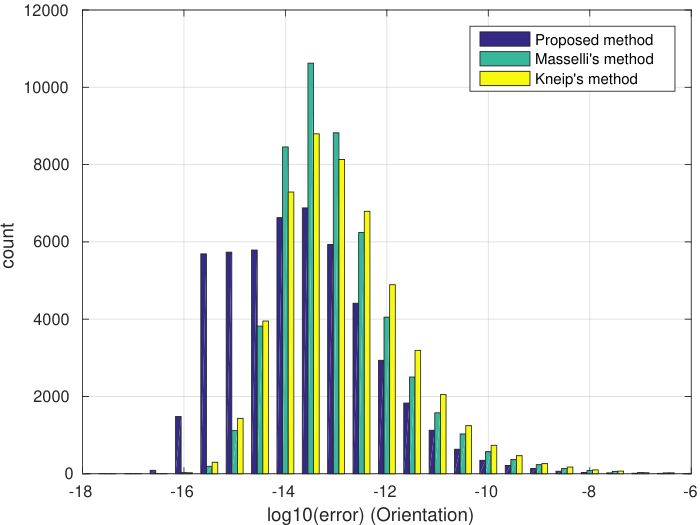
The distributions and the means of the position and orientation errors are depicted in Fig.s 3 - 4 and Table 1. As evident, we get similar results to those presented in [18] for Kneip et al.’s [15] and Masselli and Zell’s methods [18], while our approach outperforms both of them by two orders of magnitude in terms of accuracy. This can be attributed to the fact that our algorithm requires fewer operations and thus exhibits lower numerical-error propagation.

Furthermore, and as shown in the results of Table 1, we can further improve the numerical precision by applying root polishing. Typically, two iterations of Newton’s method [24] lead to significantly better results, especially for the orientation, while taking only 0.01 $\mu$ s per iteration, or about 4% of the total processing time.

	position	orientation
Kneip’s method	1.18E-05	1.02E-05
Masselli’s method	1.84E-08	4.89E-10
Proposed method	1.66E-10	5.30E-12
Proposed method+Root polishing	5.07E-11	1.53E-13

Table 1: Nominal case: Pose mean errors.

3.2 Processing cost

We use a test program that solves 100,000 randomly generated P3P problems and calculates the total execution time to evaluate the computational cost of the three algorithms considered. We run it on a 2.0 GHz $\times$ 4 Core laptop and the results show that our code takes 0.54 $\mu$ s on average (0.52 $\mu$ s without root polishing) while [15] and [18] take 1.3 $\mu$ s and 1.5 $\mu$ s, respectively. This corresponds to a 2.5 $\times$ speed up (or 40% of the time of [15]). Note also, in contrast to what is reported in [18], Masselli’s method is actually slower than Kneip’s. As mentioned earlier, Masselli’s results in [18] are based on 1,000 runs of the same features’ configuration, and take advantage of data caching to outperform Kneip.

3.3 Robustness

There are two typical singular cases that lead to infinite solutions in the P3P problem:

•

Singular case 1: The 3 landmarks are collinear.
•

Singular case 2: Any two of the 3 bearing measurements coincide.

In practice, it is almost impossible for these conditions to hold exactly, but we may still have numerical issues when the geometric configuration is close to these cases. To test the robustness of the three algorithms considered, we generate simulation data corresponding to small perturbations (uniformly distributed within $[-0.05~~0.05]$ ) of the features’ positions when in singular configurations. The errors are defined as in Section 3.1, while we compute the medians of them to assess the robustness of the three methods. For fairness, we do not apply root polishing to our code here. According to the results shown in Fig.s 5 - 8 and Tables 2 - 3, our method achieves the best accuracy in these two close-to-singular cases. The reason is that we do not compute any quantities that may suffer from numerical issues, such as cotangent and tangent in [15] and [18], respectively.

	position	orientation
Kneip’s method	1.42E-14	1.34E-14
Masselli’s method	7.13E-15	6.15E-15
Proposed method	5.16E-15	3.73E-15

Table 2: Singular case 1: Pose median errors.

	position	orientation
Kneip’s method	8.10E-14	8.85E-14
Masselli’s method	7.24E-14	6.07E-14
Proposed method	6.73E-14	1.75E-14

Table 3: Singular case 2: Pose median errors.

4 Conclusion and Future Work

In this paper, we have introduced an algebraic approach for computing the solutions of the P3P problem in closed form. Similarly to [15] and [18], our algorithm does not solve for the distances first, and hence reduces numerical-error propagation. Differently though, it does not involve numerically-unstable functions (e.g., tangent, or cotangent) and has simpler expressions than the two recent alternative methods [15, 18], and thus it outperforms them in terms of speed, accuracy, and robustness to close-to-singular cases.

As part of our ongoing work, we are currently extending our approach to also address the case of the generalized (non-central camera) P3P [20].

5 Appendix

5.1 Proof of $\mathbf{k}^{\prime}_{3}=\mathbf{k}_{2}\times\mathbf{k}_{1}$

First, note that $\mathbf{k}_{2}\times\mathbf{k}_{1}$ is a unit vector since $\mathbf{k}_{2}$ is perpendicular to $\mathbf{k}_{1}$ . Also, from (13) and (7) we have

\mathbf{k}_{1}^{\scriptscriptstyle{T}}\mathbf{k}^{\prime}_{3}=\mathbf{k}_{1}^{\scriptscriptstyle{T}}\mathbf{C}(\mathbf{k}_{2},\theta_{2})\mathbf{k}_{3}=0

(57)

Then, we can prove $\mathbf{k}^{\prime}_{3}=\mathbf{k}_{2}\times\mathbf{k}_{1}$ by showing that their inner product is equal to 1:

	$\displaystyle(\mathbf{k}_{2}\times\mathbf{k}_{1})^{\scriptscriptstyle{T}}\mathbf{k}_{3}^{\prime}$	$\displaystyle=\mathbf{k}_{1}^{\scriptscriptstyle{T}}(\mathbf{k}_{3}^{\prime}\times\mathbf{k}_{2})$
		$\displaystyle\stackrel{{\scriptstyle\eqref{eq:ki}}}{{=}}\frac{\mathbf{k}_{1}^{\scriptscriptstyle{T}}(\mathbf{k}_{3}^{\prime}\times(\mathbf{k}_{1}\times\mathbf{k}_{3}))}{\\|\mathbf{k}_{1}\times\mathbf{k}_{3}\\|}$
		$\displaystyle\stackrel{{\scriptstyle\eqref{eq:st2}}}{{=}}\frac{\mathbf{k}_{1}^{\scriptscriptstyle{T}}(\mathbf{k}_{1}(\mathbf{k}_{3}^{\scriptscriptstyle{T}}\mathbf{k}_{3}^{\prime})-\mathbf{k}_{3}(\mathbf{k}_{1}^{\scriptscriptstyle{T}}\mathbf{k}_{3}^{\prime}))}{\cos\theta_{2}}$
		$\displaystyle=\frac{\mathbf{k}_{3}^{\scriptscriptstyle{T}}\mathbf{C}(\mathbf{k}_{2},\theta_{2})\mathbf{k}_{3}}{\cos\theta_{2}}=1$

5.2 Equivalence between the two solutions of $\theta_{2}$

When solving for $\theta_{2}$ [see (9)], we have two possible solutions $\theta_{2}^{(1)}=\arccos(\mathbf{k}_{1}^{\scriptscriptstyle{T}}\mathbf{k}_{3})-\frac{\pi}{2}$ and $\theta_{2}^{(2)}=\theta_{2}^{(1)}+\pi$ . Next, we will prove that using $\theta_{2}^{(2)}$ to find ${}^{\scriptscriptstyle{G}}_{\scriptscriptstyle{C}}\mathbf{C}$ is equivalent to using $\theta_{2}^{(1)}$ . First, note that (see Fig. 2)

	$\displaystyle\mathbf{C}(\mathbf{k}_{2},\theta_{2}^{(1)}+\frac{\pi}{2})\mathbf{k}_{3}$	$\displaystyle=\mathbf{C}(\mathbf{k}_{2},\frac{\pi}{2})\mathbf{k}_{3}^{\prime}=-\mathbf{k}_{2}\times\mathbf{k}_{3}^{\prime}$
		$\displaystyle=-\mathbf{k}_{2}\times(\mathbf{k}_{2}\times\mathbf{k}_{1})=\mathbf{k}_{1}$		(58)

Then, we can write $\mathbf{C}(\mathbf{k}_{2},\theta_{2}^{(2)})$ as

	$\displaystyle\mathbf{C}(\mathbf{k}_{2},\theta_{2}^{(2)})$
$\displaystyle=$	$\displaystyle\mathbf{C}(\mathbf{k}_{2},\theta_{2}^{(1)}+\frac{\pi}{2})\mathbf{C}(\mathbf{k}_{2},\frac{\pi}{2})$
$\displaystyle=$	$\displaystyle\mathbf{C}(\mathbf{k}_{2},\theta_{2}^{(1)}+\frac{\pi}{2})\mathbf{C}(\mathbf{k}_{3},\pi)\mathbf{C}(\mathbf{k}_{2},-\frac{\pi}{2})\mathbf{C}(\mathbf{k}_{3},-\pi)$
$\displaystyle=$	$\displaystyle\mathbf{C}(\mathbf{C}(\mathbf{k}_{2},\theta_{2}^{(1)}+\frac{\pi}{2})\mathbf{k}_{3},\pi)\mathbf{C}(\mathbf{k}_{2},\theta_{2}^{(1)}+\frac{\pi}{2})\mathbf{C}(\mathbf{k}_{2},-\frac{\pi}{2})\mathbf{C}(\mathbf{k}_{3},\pi)$
$\displaystyle\stackrel{{\scriptstyle\eqref{eq:t290}}}{{=}}$	$\displaystyle\mathbf{C}(\mathbf{k}_{1},\pi)\mathbf{C}(\mathbf{k}_{2},\theta_{2}^{(1)})\mathbf{C}(\mathbf{k}_{3},\pi)$	(59)

If we use $\theta_{2}^{(2)}$ to find ${}^{\scriptscriptstyle{G}}_{\scriptscriptstyle{C}}\mathbf{C}$ ,

$\displaystyle{}^{\scriptscriptstyle{G}}_{\scriptscriptstyle{C}}\mathbf{C}$	$\displaystyle=\mathbf{C}(\mathbf{k}_{1},\theta_{1}^{(2)})\mathbf{C}(\mathbf{k}_{2},\theta_{2}^{(2)})\mathbf{C}(\mathbf{k}_{3},\theta_{3}^{(2)})$
	$\displaystyle\stackrel{{\scriptstyle\eqref{eq:ck2}}}{{=}}\mathbf{C}(\mathbf{k}_{1},\theta_{1}^{(2)})\mathbf{C}(\mathbf{k}_{1},\pi)\mathbf{C}(\mathbf{k}_{2},\theta_{2}^{(1)})\mathbf{C}(\mathbf{k}_{3},\pi)\mathbf{C}(\mathbf{k}_{3},\theta_{3}^{(2)})$
	$\displaystyle=\mathbf{C}(\mathbf{k}_{1},\theta_{1}^{(2)}+\pi)\mathbf{C}(\mathbf{k}_{2},\theta_{2}^{(1)})\mathbf{C}(\mathbf{k}_{3},\theta_{3}^{(2)}+\pi)$	(60)

Note that ${}^{\scriptscriptstyle{G}}_{\scriptscriptstyle{C}}\mathbf{C}$ in (60) is of the same form as that in (5), so any solutions of ${}^{\scriptscriptstyle{G}}_{\scriptscriptstyle{C}}\mathbf{C}$ computed using $\theta_{2}^{(2)}$ will be found by using $\theta_{2}^{(1)}$ . Thus, we do not need to consider any other solutions for $\theta_{1}$ and $\theta_{3}$ beyond the ones found for ${}^{\scriptscriptstyle{G}}_{\scriptscriptstyle{C}}\mathbf{C}$ .

5.3 Determining the sign of $\sin\theta_{1}^{\prime}$

From (51), we have two solutions for $\sin\theta_{1}^{\prime}$ , and thus for $\theta_{1}^{\prime}$ , with $\theta_{1}^{\prime(2)}=-\theta_{1}^{\prime}$ . This will also result into two solutions for $\theta_{3}^{\prime}$ [see (52)] and, hence, two solutions for $\theta_{3}$ : $\theta_{3}$ and $\theta_{3}^{(2)}=\theta_{3}+\pi$ . Considering these two options, we get two distinct solutions for ${}^{\scriptscriptstyle{G}}_{\scriptscriptstyle{C}}\mathbf{C}$ [see (53)]:

	$\displaystyle\mathbf{C}_{1}$	$\displaystyle\triangleq\mathbf{C}(\mathbf{k}_{1},\theta_{1}^{\prime})\mathbf{C}(\mathbf{k}_{3}^{\prime\prime},\theta_{3})\mathbf{C}(\mathbf{k}_{1},\phi)\mathbf{C}(\mathbf{k}_{2},\theta_{2})$
	$\displaystyle\mathbf{C}_{2}$	$\displaystyle\triangleq\mathbf{C}(\mathbf{k}_{1},-\theta_{1}^{\prime})\mathbf{C}(\mathbf{k}_{3}^{\prime\prime},\theta_{3}+\pi)\mathbf{C}(\mathbf{k}_{1},\phi)\mathbf{C}(\mathbf{k}_{2},\theta_{2})$

Then, notice that

	$\displaystyle\mathbf{C}_{2}\mathbf{C}_{1}^{\scriptscriptstyle{T}}$	$\displaystyle=\mathbf{C}(\mathbf{k}_{1},-\theta_{1}^{\prime})\mathbf{C}(\mathbf{k}_{3}^{\prime\prime},\pi)\mathbf{C}(\mathbf{k}_{1},-\theta_{1}^{\prime})$
		$\displaystyle=\mathbf{C}(\mathbf{k}_{3}^{\prime\prime},\pi)\mathbf{C}(\mathbf{C}^{\scriptscriptstyle{T}}(\mathbf{k}_{3}^{\prime\prime},\pi)\mathbf{k}_{1},-\theta_{1}^{\prime})\mathbf{C}(\mathbf{k}_{1},-\theta_{1}^{\prime})$
		$\displaystyle=\mathbf{C}(\mathbf{k}_{3}^{\prime\prime},\pi)\mathbf{C}(-\mathbf{k}_{1},-\theta_{1}^{\prime})\mathbf{C}(\mathbf{k}_{1},-\theta_{1}^{\prime})$
		$\displaystyle=\mathbf{C}(\mathbf{k}_{3}^{\prime\prime},\pi)$

If $\mathbf{C}_{1}=\mathbf{C}_{2}$ , this would require

\displaystyle\mathbf{C}(\mathbf{k}_{3}^{\prime\prime},\pi)=\mathbf{C}_{2}\mathbf{C}_{1}^{\scriptscriptstyle{T}}=\mathbf{I}

which cannot be true, hence $\mathbf{C}_{1}$ and $\mathbf{C}_{2}$ cannot be equal. Thus, there are always two different solutions of ${}^{\scriptscriptstyle{G}}_{\scriptscriptstyle{C}}\mathbf{C}$ .

If, however, we use the fact that $d_{i}\ (i=1,2,3)$ is positive, we can determine the sign of $\sin\theta_{1}^{\prime}$ , and choose the valid one among the two solutions of ${}^{\scriptscriptstyle{G}}_{\scriptscriptstyle{C}}\mathbf{C}$ . Subtracting (1) pairwise for ( $i=3$ ) from ( $i=1$ ), we have

$\displaystyle{}^{\scriptscriptstyle{G}}\mathbf{p}_{1}-{}^{\scriptscriptstyle{G}}\mathbf{p}_{3}=$	$\displaystyle d_{1}{}^{\scriptscriptstyle{G}}_{\scriptscriptstyle{C}}\mathbf{C}{}^{\scriptscriptstyle{C}}\mathbf{b}_{1}-d_{3}{}^{\scriptscriptstyle{G}}_{\scriptscriptstyle{C}}\mathbf{C}{}^{\scriptscriptstyle{C}}\mathbf{b}_{3}$
$\displaystyle\Rightarrow{}^{\scriptscriptstyle{G}}\mathbf{p}_{1}-{}^{\scriptscriptstyle{G}}\mathbf{p}_{3}=$	$\displaystyle\mathbf{C}(\mathbf{k}_{1},\theta_{1}^{\prime})\mathbf{C}(\mathbf{k}_{3}^{\prime\prime},\theta_{3})\mathbf{C}(\mathbf{k}_{1},\phi)$
$\displaystyle\cdot$	$\displaystyle\mathbf{C}(\mathbf{k}_{2},\theta_{2})(d_{1}{}^{\scriptscriptstyle{C}}\mathbf{b}_{1}-d_{3}{}^{\scriptscriptstyle{C}}\mathbf{b}_{3})$	(61)

Multiplying both sides of (61) with ${\mathbf{k}_{3}^{\prime\prime}}^{\scriptscriptstyle{T}}\mathbf{C}(\mathbf{k}_{1},-\theta_{1}^{\prime})$ from the left, yields

	$\displaystyle{\mathbf{k}_{3}^{\prime\prime}}^{\scriptscriptstyle{T}}\mathbf{C}(\mathbf{k}_{1},-\theta_{1}^{\prime})({}^{\scriptscriptstyle{G}}\mathbf{p}_{1}-{}^{\scriptscriptstyle{G}}\mathbf{p}_{3})$
$\displaystyle=$	$\displaystyle{\mathbf{k}_{3}^{\prime\prime}}^{\scriptscriptstyle{T}}\mathbf{C}(\mathbf{k}_{1},\phi)\mathbf{C}(\mathbf{k}_{2},\theta_{2})(d_{1}{}^{\scriptscriptstyle{C}}\mathbf{b}_{1}-d_{3}{}^{\scriptscriptstyle{C}}\mathbf{b}_{3})$
$\displaystyle\Rightarrow$	$\displaystyle{\mathbf{k}_{3}^{\prime\prime}}^{\scriptscriptstyle{T}}(\cos\theta_{1}^{\prime}\mathbf{I}+\sin\theta_{1}^{\prime}\lfloor\mathbf{k}_{1}\rfloor+(1-\cos\theta_{1}^{\prime})\mathbf{k}_{1}\mathbf{k}_{1}^{\scriptscriptstyle{T}})\mathbf{u}_{1}$
$\displaystyle=$	$\displaystyle{\mathbf{k}_{3}^{\prime}}^{\scriptscriptstyle{T}}\mathbf{C}(\mathbf{k}_{2},\theta_{2})(d_{1}{}^{\scriptscriptstyle{C}}\mathbf{b}_{1}-d_{3}{}^{\scriptscriptstyle{C}}\mathbf{b}_{3})$
$\displaystyle\stackrel{{\scriptstyle\eqref{eq:k3pp}}}{{\Rightarrow}}$	$\displaystyle\sin\theta_{1}^{\prime}{\mathbf{k}_{3}^{\prime\prime}}^{\scriptscriptstyle{T}}\lfloor\mathbf{k}_{1}\rfloor\mathbf{u}_{1}=\mathbf{k}_{3}^{\scriptscriptstyle{T}}(d_{1}{}^{\scriptscriptstyle{C}}\mathbf{b}_{1}-d_{3}{}^{\scriptscriptstyle{C}}\mathbf{b}_{3})$
$\displaystyle\Rightarrow$	$\displaystyle-\sin\theta_{1}^{\prime}\mathbf{u}_{1}^{\scriptscriptstyle{T}}\lfloor\mathbf{k}_{1}\rfloor\mathbf{k}_{3}^{\prime\prime}=-d_{3}\mathbf{k}_{3}^{\scriptscriptstyle{T}}{}^{\scriptscriptstyle{C}}\mathbf{b}_{3}$
$\displaystyle\Rightarrow$	$\displaystyle\delta\sin\theta_{1}^{\prime}=d_{3}(\mathbf{k}_{3}^{\scriptscriptstyle{T}}{}^{\scriptscriptstyle{C}}\mathbf{b}_{3})$	(62)

Using the fact that $d_{3}>0$ and $\delta>0$ , we select the sign of $\sin\theta_{1}^{\prime}$ to be the same as that of $\mathbf{k}_{3}^{\scriptscriptstyle{T}}{}^{\scriptscriptstyle{C}}\mathbf{b}_{3}$ .

5.4 Least-squares solution for the position

${}^{\scriptscriptstyle{G}}\mathbf{p}_{\scriptscriptstyle{C}}$ can also be solved following a least-squares approach, which is slower but more accurate than (56). Specifically, (1) can result in the following system:

\begin{bmatrix}{}^{\scriptscriptstyle{G}}\mathbf{C}_{\scriptscriptstyle{C}}{}^{\scriptscriptstyle{C}}\mathbf{b}_{1}&&&\mathbf{I}\\ &{}^{\scriptscriptstyle{G}}\mathbf{C}_{\scriptscriptstyle{C}}{}^{\scriptscriptstyle{C}}\mathbf{b}_{2}&&\mathbf{I}\\ &&{}^{\scriptscriptstyle{G}}\mathbf{C}_{\scriptscriptstyle{C}}{}^{\scriptscriptstyle{C}}\mathbf{b}_{3}&\mathbf{I}\\ \end{bmatrix}\begin{bmatrix}d_{1}\\ d_{2}\\ d_{3}\\ {}^{\scriptscriptstyle{G}}\mathbf{p}_{\scriptscriptstyle{C}}\end{bmatrix}=\begin{bmatrix}{}^{\scriptscriptstyle{G}}\mathbf{p}_{1}\\ {}^{\scriptscriptstyle{G}}\mathbf{p}_{2}\\ {}^{\scriptscriptstyle{G}}\mathbf{p}_{3}\\ \end{bmatrix}

Then, we only need to apply QR decomposition [7] and backsolve for ${}^{\scriptscriptstyle{G}}\mathbf{p}_{\scriptscriptstyle{C}}$ (i.e., we do not need to compute $d_{i},\ i=1,2,3$ ).

5.5 Derivation of $\bar{f}_{ij}$

	$\displaystyle\bar{f}_{i1}$	$\displaystyle\triangleq\mathbf{u}_{i}^{\scriptscriptstyle{T}}\lfloor\mathbf{k}_{1}\rfloor^{2}\lfloor\mathbf{k}^{\prime\prime}_{3}\rfloor^{2}\mathbf{v}^{\prime\prime}_{i}$
		$\displaystyle=\mathbf{u}_{i}^{\scriptscriptstyle{T}}\lfloor\mathbf{k}_{1}\rfloor(\mathbf{k}^{\prime\prime}_{3}\mathbf{k}_{1}^{\scriptscriptstyle{T}}-(\mathbf{k}_{1}^{\scriptscriptstyle{T}}\mathbf{k}^{\prime\prime}_{3})\mathbf{I})\lfloor\mathbf{k}^{\prime\prime}_{3}\rfloor\mathbf{v}^{\prime\prime}_{i}$
		$\displaystyle=(\mathbf{u}_{i}^{\scriptscriptstyle{T}}\lfloor\mathbf{k}_{1}\rfloor\mathbf{k}^{\prime\prime}_{3})(\mathbf{k}_{1}^{\scriptscriptstyle{T}}\lfloor\mathbf{k}^{\prime\prime}_{3}\rfloor\mathbf{v}^{\prime\prime}_{i})$
		$\displaystyle=((\mathbf{u}_{i}\times\mathbf{k}_{1})^{\scriptscriptstyle{T}}\mathbf{k}^{\prime\prime}_{3})(\mathbf{k}_{1}^{\scriptscriptstyle{T}}\mathbf{C}(\mathbf{k}_{1},\phi)\mathbf{C}(\mathbf{k}_{2},\theta_{2})\lfloor\mathbf{k}_{3}\rfloor\mathbf{v}_{i})$
		$\displaystyle=\delta{\mathbf{k}_{1}^{\prime}}^{\scriptscriptstyle{T}}\lfloor\mathbf{k}_{3}\rfloor\mathbf{v}_{i}$
		$\displaystyle=\delta\mathbf{v}_{i}^{\scriptscriptstyle{T}}\mathbf{k}_{2}$
	$\displaystyle\bar{f}_{i2}$	$\displaystyle\triangleq\mathbf{u}_{i}^{\scriptscriptstyle{T}}\lfloor\mathbf{k}_{1}\rfloor^{2}\lfloor\mathbf{k}^{\prime\prime}_{3}\rfloor\mathbf{v}^{\prime\prime}_{i}$
		$\displaystyle=(\mathbf{u}_{i}^{\scriptscriptstyle{T}}\lfloor\mathbf{k}_{1}\rfloor\mathbf{k}^{\prime\prime}_{3})(\mathbf{k}_{1}^{\scriptscriptstyle{T}}\mathbf{v}^{\prime\prime}_{i})$
		$\displaystyle=\delta(\mathbf{k}_{1}^{\scriptscriptstyle{T}}\mathbf{C}(\mathbf{k}_{1},\phi)\mathbf{C}(\mathbf{k}_{2},\theta_{2})\mathbf{v}_{i})$
		$\displaystyle=\delta\mathbf{v}_{i}^{\scriptscriptstyle{T}}\mathbf{k}_{1}^{\prime}$
	$\displaystyle\bar{f}_{i3}$	$\displaystyle\triangleq({\mathbf{k}^{\prime\prime}_{3}}^{\scriptscriptstyle{T}}\mathbf{v}^{\prime\prime}_{i})\mathbf{u}_{i}^{\scriptscriptstyle{T}}\lfloor\mathbf{k}_{1}\rfloor\mathbf{k}^{\prime\prime}_{3}$
		$\displaystyle=\delta\mathbf{k}_{3}^{\scriptscriptstyle{T}}\mathbf{C}(\mathbf{k}_{2},-\theta_{2})\mathbf{C}(\mathbf{k}_{1},-\phi)\mathbf{C}(\mathbf{k}_{1},\phi)\mathbf{C}(\mathbf{k}_{2},\theta_{2})\mathbf{v}_{i}$
		$\displaystyle=\delta\mathbf{v}_{i}^{\scriptscriptstyle{T}}\mathbf{k}_{3}$
	$\displaystyle\bar{f}_{i4}$	$\displaystyle\triangleq-(\mathbf{u}_{i}^{\scriptscriptstyle{T}}\mathbf{k}_{1})\mathbf{k}_{1}^{\scriptscriptstyle{T}}\lfloor\mathbf{k}^{\prime\prime}_{3}\rfloor^{2}\mathbf{v}^{\prime\prime}_{i}$
		$\displaystyle=-(\mathbf{u}_{i}^{\scriptscriptstyle{T}}\mathbf{k}_{1})\mathbf{k}_{1}(\mathbf{k}^{\prime\prime}_{3}{\mathbf{k}^{\prime\prime}_{3}}^{\scriptscriptstyle{T}}-\mathbf{I})\mathbf{v}^{\prime\prime}_{i}$
		$\displaystyle=(\mathbf{u}_{i}^{\scriptscriptstyle{T}}\mathbf{k}_{1})(\mathbf{k}_{1}\mathbf{v}^{\prime\prime}_{i})$
		$\displaystyle=(\mathbf{u}_{i}^{\scriptscriptstyle{T}}\mathbf{k}_{1})(\mathbf{v}_{i}^{\scriptscriptstyle{T}}\mathbf{k}_{1}^{\prime})$
	$\displaystyle\bar{f}_{i5}$	$\displaystyle\triangleq-(\mathbf{u}_{i}^{\scriptscriptstyle{T}}\mathbf{k}_{1})\mathbf{k}_{1}^{\scriptscriptstyle{T}}\lfloor\mathbf{k}^{\prime\prime}_{3}\rfloor\mathbf{v}^{\prime\prime}_{i}=-(\mathbf{u}_{i}^{\scriptscriptstyle{T}}\mathbf{k}_{1})(\mathbf{v}_{i}^{\scriptscriptstyle{T}}\mathbf{k}_{2})$

5.6 Derivation of $f_{ij}$ and $\bar{\bar{\mathbf{C}}}$

First, note that

	$\displaystyle\mathbf{v}_{i}^{\scriptscriptstyle{T}}\mathbf{k}_{2}$	$\displaystyle=({}^{\scriptscriptstyle{C}}\mathbf{b}_{i}\times{}^{\scriptscriptstyle{C}}\mathbf{b}_{3})^{\scriptscriptstyle{T}}(\mathbf{k}_{1}^{\prime}\times\mathbf{k}_{3})$
		$\displaystyle=({}^{\scriptscriptstyle{C}}\mathbf{b}_{i}^{\scriptscriptstyle{T}}\mathbf{k}_{1}^{\prime})({}^{\scriptscriptstyle{C}}\mathbf{b}_{3}^{\scriptscriptstyle{T}}\mathbf{k}_{3})-({}^{\scriptscriptstyle{C}}\mathbf{b}_{i}^{\scriptscriptstyle{T}}\mathbf{k}_{3})({}^{\scriptscriptstyle{C}}\mathbf{b}_{3}^{\scriptscriptstyle{T}}\mathbf{k}_{1}^{\prime})$
		$\displaystyle=({}^{\scriptscriptstyle{C}}\mathbf{b}_{i}^{\scriptscriptstyle{T}}\mathbf{k}_{1}^{\prime})({}^{\scriptscriptstyle{C}}\mathbf{b}_{3}^{\scriptscriptstyle{T}}\mathbf{k}_{3})$
	$\displaystyle\mathbf{v}_{i}^{\scriptscriptstyle{T}}\mathbf{k}_{1}^{\prime}$	$\displaystyle=-({}^{\scriptscriptstyle{C}}\mathbf{b}_{i}\times{}^{\scriptscriptstyle{C}}\mathbf{b}_{3})^{\scriptscriptstyle{T}}(\mathbf{k}_{2}\times\mathbf{k}_{3})$
		$\displaystyle=-({}^{\scriptscriptstyle{C}}\mathbf{b}_{i}^{\scriptscriptstyle{T}}\mathbf{k}_{2})({}^{\scriptscriptstyle{C}}\mathbf{b}_{3}^{\scriptscriptstyle{T}}\mathbf{k}_{3})+({}^{\scriptscriptstyle{C}}\mathbf{b}_{i}^{\scriptscriptstyle{T}}\mathbf{k}_{3})({}^{\scriptscriptstyle{C}}\mathbf{b}_{3}^{\scriptscriptstyle{T}}\mathbf{k}_{2})$
		$\displaystyle=-({}^{\scriptscriptstyle{C}}\mathbf{b}_{i}^{\scriptscriptstyle{T}}\mathbf{k}_{2})({}^{\scriptscriptstyle{C}}\mathbf{b}_{3}^{\scriptscriptstyle{T}}\mathbf{k}_{3})$

Let $\psi\triangleq\theta_{3}-\theta_{3}^{\prime}$ , and thus

\displaystyle\begin{bmatrix}\cos\theta_{3}^{\prime}\\ \sin\theta_{3}^{\prime}\end{bmatrix}=\begin{bmatrix}\cos\psi\cos\theta_{3}+\sin\psi\sin\theta_{3}\\ \cos\psi\cos\theta_{3}+\sin\psi\sin\theta_{3}\end{bmatrix}

(63)

From (63) and (27), we get

	$\displaystyle\cos\psi$	$\displaystyle=\frac{\bar{f}_{11}}{\sqrt{\bar{f}_{11}^{2}+\bar{f}_{12}^{2}}}=-\frac{\bar{f}_{15}}{\sqrt{\bar{f}_{14}^{2}+\bar{f}_{15}^{2}}}$
		$\displaystyle=\frac{\mathbf{v}_{1}^{\scriptscriptstyle{T}}\mathbf{k}_{2}}{\sqrt{(\mathbf{v}_{1}^{\scriptscriptstyle{T}}\mathbf{k}_{2})^{2}+(\mathbf{v}_{1}^{\scriptscriptstyle{T}}\mathbf{k}_{1}^{\prime})^{2}}}$
		$\displaystyle=\frac{{}^{\scriptscriptstyle{C}}\mathbf{b}_{1}^{\scriptscriptstyle{T}}\mathbf{k}_{1}^{\prime}}{\sqrt{({}^{\scriptscriptstyle{C}}\mathbf{b}_{1}^{\scriptscriptstyle{T}}\mathbf{k}_{2})^{2}+({}^{\scriptscriptstyle{C}}\mathbf{b}_{1}^{\scriptscriptstyle{T}}\mathbf{k}_{1}^{\prime})^{2}}}$
		$\displaystyle=\frac{{}^{\scriptscriptstyle{C}}\mathbf{b}_{1}^{\scriptscriptstyle{T}}\mathbf{k}_{1}^{\prime}}{\\|\mathbf{k}_{3}\times{}^{\scriptscriptstyle{C}}\mathbf{b}_{1}\\|}$
		$\displaystyle={}^{\scriptscriptstyle{C}}\mathbf{b}_{1}^{\scriptscriptstyle{T}}\mathbf{k}_{1}^{\prime}$

	$\displaystyle\sin\psi$	$\displaystyle=\frac{\bar{f}_{12}}{\sqrt{\bar{f}_{11}^{2}+\bar{f}_{12}^{2}}}=\frac{\bar{f}_{14}}{\sqrt{\bar{f}_{14}^{2}+\bar{f}_{15}^{2}}}$
		$\displaystyle=\frac{\mathbf{v}_{1}^{\scriptscriptstyle{T}}\mathbf{k}_{1}^{\prime}}{\sqrt{(\mathbf{v}_{1}^{\scriptscriptstyle{T}}\mathbf{k}_{2})^{2}+(\mathbf{v}_{1}^{\scriptscriptstyle{T}}\mathbf{k}_{1}^{\prime})^{2}}}$
		$\displaystyle=-{}^{\scriptscriptstyle{C}}\mathbf{b}_{1}^{\scriptscriptstyle{T}}\mathbf{k}_{2}$

Then, from (26) and (28), we derive the expressions of $f_{ij}$ :

	$\displaystyle f_{11}$	$\displaystyle=\bar{f}_{11}\cos\psi+\bar{f}_{12}\sin\psi$
		$\displaystyle=\delta({}^{\scriptscriptstyle{C}}\mathbf{b}_{3}^{\scriptscriptstyle{T}}\mathbf{k}_{3})(({}^{\scriptscriptstyle{C}}\mathbf{b}_{1}^{\scriptscriptstyle{T}}\mathbf{k}_{2})^{2}+({}^{\scriptscriptstyle{C}}\mathbf{b}_{1}^{\scriptscriptstyle{T}}\mathbf{k}_{1}^{\prime})^{2})$
		$\displaystyle=\delta({}^{\scriptscriptstyle{C}}\mathbf{b}_{3}^{\scriptscriptstyle{T}}\mathbf{k}_{3})$
	$\displaystyle f_{21}$	$\displaystyle=\bar{f}_{21}\cos\psi+\bar{f}_{22}\sin\psi$
		$\displaystyle=\delta({}^{\scriptscriptstyle{C}}\mathbf{b}_{3}^{\scriptscriptstyle{T}}\mathbf{k}_{3})(({}^{\scriptscriptstyle{C}}\mathbf{b}_{2}^{\scriptscriptstyle{T}}\mathbf{k}_{2})({}^{\scriptscriptstyle{C}}\mathbf{b}_{1}^{\scriptscriptstyle{T}}\mathbf{k}_{2})+({}^{\scriptscriptstyle{C}}\mathbf{b}_{2}^{\scriptscriptstyle{T}}\mathbf{k}_{1}^{\prime})({}^{\scriptscriptstyle{C}}\mathbf{b}_{1}^{\scriptscriptstyle{T}}\mathbf{k}_{1}^{\prime}))$
		$\displaystyle=\delta({}^{\scriptscriptstyle{C}}\mathbf{b}_{3}^{\scriptscriptstyle{T}}\mathbf{k}_{3})({}^{\scriptscriptstyle{C}}\mathbf{b}_{2}^{\scriptscriptstyle{T}}(\mathbf{k}_{2}\mathbf{k}_{2}^{\scriptscriptstyle{T}}+\mathbf{k}_{1}^{\prime}{\mathbf{k}_{1}^{\prime}}^{\scriptscriptstyle{T}}){}^{\scriptscriptstyle{C}}\mathbf{b}_{1})$
		$\displaystyle=\delta({}^{\scriptscriptstyle{C}}\mathbf{b}_{3}^{\scriptscriptstyle{T}}\mathbf{k}_{3})({}^{\scriptscriptstyle{C}}\mathbf{b}_{2}^{\scriptscriptstyle{T}}(\mathbf{I}-\mathbf{k}_{3}\mathbf{k}_{3}^{\scriptscriptstyle{T}}){}^{\scriptscriptstyle{C}}\mathbf{b}_{1})$
		$\displaystyle=\delta({}^{\scriptscriptstyle{C}}\mathbf{b}_{3}^{\scriptscriptstyle{T}}\mathbf{k}_{3})({}^{\scriptscriptstyle{C}}\mathbf{b}_{2}^{\scriptscriptstyle{T}}{}^{\scriptscriptstyle{C}}\mathbf{b}_{1})$
	$\displaystyle f_{22}$	$\displaystyle=-\bar{f}_{21}\sin\psi+\bar{f}_{22}\cos\psi$
		$\displaystyle=\delta({}^{\scriptscriptstyle{C}}\mathbf{b}_{3}^{\scriptscriptstyle{T}}\mathbf{k}_{3})(({}^{\scriptscriptstyle{C}}\mathbf{b}_{2}^{\scriptscriptstyle{T}}\mathbf{k}_{1}^{\prime})({}^{\scriptscriptstyle{C}}\mathbf{b}_{1}^{\scriptscriptstyle{T}}\mathbf{k}_{2})-({}^{\scriptscriptstyle{C}}\mathbf{b}_{2}^{\scriptscriptstyle{T}}\mathbf{k}_{2})({}^{\scriptscriptstyle{C}}\mathbf{b}_{1}^{\scriptscriptstyle{T}}\mathbf{k}_{1}^{\prime}))$
		$\displaystyle=\delta({}^{\scriptscriptstyle{C}}\mathbf{b}_{3}^{\scriptscriptstyle{T}}\mathbf{k}_{3})({}^{\scriptscriptstyle{C}}\mathbf{b}_{2}^{\scriptscriptstyle{T}}(\mathbf{k}_{2}\mathbf{k}_{2}^{\scriptscriptstyle{T}}+\mathbf{k}_{1}^{\prime}{\mathbf{k}_{1}^{\prime}}^{\scriptscriptstyle{T}}){}^{\scriptscriptstyle{C}}\mathbf{b}_{1})$
		$\displaystyle=\delta({}^{\scriptscriptstyle{C}}\mathbf{b}_{3}^{\scriptscriptstyle{T}}\mathbf{k}_{3})({}^{\scriptscriptstyle{C}}\mathbf{b}_{2}\times{}^{\scriptscriptstyle{C}}\mathbf{b}_{1})^{\scriptscriptstyle{T}}(\mathbf{k}_{1}^{\prime}\times\mathbf{k}_{2})$
		$\displaystyle=\delta({}^{\scriptscriptstyle{C}}\mathbf{b}_{3}^{\scriptscriptstyle{T}}\mathbf{k}_{3})\\|{}^{\scriptscriptstyle{C}}\mathbf{b}_{2}\times{}^{\scriptscriptstyle{C}}\mathbf{b}_{1}\\|\mathbf{k}_{3}^{\scriptscriptstyle{T}}\mathbf{k}_{3}$
		$\displaystyle=\delta({}^{\scriptscriptstyle{C}}\mathbf{b}_{3}^{\scriptscriptstyle{T}}\mathbf{k}_{3})\\|{}^{\scriptscriptstyle{C}}\mathbf{b}_{2}\times{}^{\scriptscriptstyle{C}}\mathbf{b}_{1}\\|$
	$\displaystyle f_{15}$	$\displaystyle=\bar{f}_{15}\cos\psi-\bar{f}_{14}\sin\psi$
		$\displaystyle=-(\mathbf{u}_{1}^{\scriptscriptstyle{T}}\mathbf{k}_{1})f_{11}/\delta$
		$\displaystyle=-(\mathbf{u}_{1}^{\scriptscriptstyle{T}}\mathbf{k}_{1})({}^{\scriptscriptstyle{C}}\mathbf{b}_{3}^{\scriptscriptstyle{T}}\mathbf{k}_{3})$
	$\displaystyle f_{24}$	$\displaystyle=\bar{f}_{25}\sin\psi+\bar{f}_{24}\cos\psi$
		$\displaystyle=(\mathbf{u}_{2}^{\scriptscriptstyle{T}}\mathbf{k}_{1})f_{22}/\delta$
		$\displaystyle=(\mathbf{u}_{2}^{\scriptscriptstyle{T}}\mathbf{k}_{1})({}^{\scriptscriptstyle{C}}\mathbf{b}_{3}^{\scriptscriptstyle{T}}\mathbf{k}_{3})\\|{}^{\scriptscriptstyle{C}}\mathbf{b}_{2}\times{}^{\scriptscriptstyle{C}}\mathbf{b}_{1}\\|$
	$\displaystyle f_{25}$	$\displaystyle=\bar{f}_{25}\cos\psi-\bar{f}_{24}\sin\psi$
		$\displaystyle=-(\mathbf{u}_{2}^{\scriptscriptstyle{T}}\mathbf{k}_{1})f_{21}/\delta$
		$\displaystyle=-(\mathbf{u}_{2}^{\scriptscriptstyle{T}}\mathbf{k}_{1})({}^{\scriptscriptstyle{C}}\mathbf{b}_{3}^{\scriptscriptstyle{T}}\mathbf{k}_{3})({}^{\scriptscriptstyle{C}}\mathbf{b}_{1}^{\scriptscriptstyle{T}}\mathbf{k}_{1}^{\prime})$

Additionally, we can derive the expression of $\mathbf{\bar{\bar{C}}}$ , which is defined in (55):

	$\displaystyle\mathbf{\bar{\bar{C}}}$	$\displaystyle=\mathbf{C}(\mathbf{e}_{2},\theta_{3}-\theta_{3}^{\prime})\mathbf{\bar{C}}^{\scriptscriptstyle{T}}\mathbf{C}(\mathbf{k}_{1},\phi)\mathbf{C}(\mathbf{k}_{2},\theta_{2})$
		$\displaystyle=\mathbf{C}(\mathbf{e}_{2},\psi)\begin{bmatrix}\mathbf{k}_{1}&\mathbf{k}_{3}^{\prime}&\mathbf{k}_{2}\end{bmatrix}^{\scriptscriptstyle{T}}\mathbf{C}(\mathbf{k}_{2},\theta_{2})$
		$\displaystyle=\mathbf{C}(\mathbf{e}_{2},\psi)\begin{bmatrix}\mathbf{k}_{1}^{\prime}&\mathbf{k}_{3}&\mathbf{k}_{2}\end{bmatrix}^{\scriptscriptstyle{T}}$
		$\displaystyle=\begin{bmatrix}\cos\psi\mathbf{k}_{1}^{\prime}-\sin\psi\mathbf{k}_{2}&\mathbf{k}_{3}&\sin\psi\mathbf{k}_{1}^{\prime}+\cos\psi\mathbf{k}_{2}\end{bmatrix}^{\scriptscriptstyle{T}}$
		$\displaystyle=\begin{bmatrix}(\mathbf{k}_{1}^{\prime}{\mathbf{k}_{1}^{\prime}}^{\scriptscriptstyle{T}}+\mathbf{k}_{2}\mathbf{k}_{2}^{\scriptscriptstyle{T}}){}^{\scriptscriptstyle{C}}\mathbf{b}_{1}&\mathbf{k}_{3}&\sin\psi\mathbf{k}_{1}^{\prime}+\cos\psi\mathbf{k}_{2}\end{bmatrix}^{\scriptscriptstyle{T}}$
		$\displaystyle=\begin{bmatrix}(\mathbf{I}-\mathbf{k}_{3}\mathbf{k}_{3}^{\scriptscriptstyle{T}}){}^{\scriptscriptstyle{C}}\mathbf{b}_{1}&\mathbf{k}_{3}&\sin\psi\mathbf{k}_{1}^{\prime}+\cos\psi\mathbf{k}_{2}\end{bmatrix}^{\scriptscriptstyle{T}}$
		$\displaystyle=\begin{bmatrix}{}^{\scriptscriptstyle{C}}\mathbf{b}_{1}&\mathbf{k}_{3}&\sin\psi\mathbf{k}_{1}^{\prime}+\cos\psi\mathbf{k}_{2}\end{bmatrix}^{\scriptscriptstyle{T}}$
		$\displaystyle=\begin{bmatrix}{}^{\scriptscriptstyle{C}}\mathbf{b}_{1}&\mathbf{k}_{3}&{}^{\scriptscriptstyle{C}}\mathbf{b}_{1}\times\mathbf{k}_{3}\end{bmatrix}^{\scriptscriptstyle{T}}$

5.7 Comparison with the P3P code in OpenCV

We also compared the performance of our code with that in OpenCV (based on [6]), using the same setup as Sec. 3. The error distributions are showed in Fig. 9 and Fig. 10. It is obvious that the code in OpenCV has lower numerical accuracy comparing to ours. Also, it takes around 3 $\mu$ s on average to compute P3P once, which is much slower than ours (0.52 $\mu$ s according to Sec. 3).

In conclusion, our code performs much better than the one in OpenCV.

References

[1] A. Ansar and K. Daniilidis. Linear pose estimation from points or lines. IEEE Transactions on Pattern Analysis and Machine Intelligence, 25(5):578–589, 2003.
[2] G. Cardano, T. R. Witmer, and O. Ore. The Rules of Algebra: Ars Magna, volume 685. Courier Corporation, 2007.
[3] D. A. Cox, J. Little, and D. O’Shea. Using algebraic geometry, volume 185. Springer Science & Business Media, 2006.
[4] S. Finsterwalder and W. Scheufele. Das rückwärtseinschneiden im raum. Verlag d. Bayer. Akad. d. Wiss., 1903.
[5] M. A. Fischler and R. C. Bolles. Random sample consensus: a paradigm for model fitting with applications to image analysis and automated cartography. Communications of the ACM, 24(6):381–395, 1981.
[6] X.-S. Gao, X.-R. Hou, J. Tang, and H.-F. Cheng. Complete solution classification for the perspective-three-point problem. IEEE Transactions on Pattern Analysis and Machine Intelligence, 25(8):930–943, 2003.
[7] G. H. Golub and C. F. Van Loan. Matrix computations, volume 3. JHU Press, 2012.
[8] E. W. Grafarend, P. Lohse, and B. Schaffrin. Dreidimensionaler rückwärtsschnitt teil i: Die projektiven gleichungen. Zeitschrift für Vermessungswesen, pages 1–37, 1989.
[9] J. A. Grunert. Das pothenotische problem in erweiterter gestalt nebst über seine anwendungen in der geodäsie. Grunerts archiv für mathematik und physik, 1:238–248, 1841.
[10] R. M. Haralick, H. Joo, C.-N. Lee, X. Zhuang, V. G. Vaidya, and M. B. Kim. Pose estimation from corresponding point data. IEEE Transactions on Systems, Man, and Cybernetics, 19(6):1426–1446, 1989.
[11] R. M. Haralick, D. Lee, K. Ottenburg, and M. Nolle. Analysis and solutions of the three point perspective pose estimation problem. In Proc. of the IEEE Conference on Computer Vision and Pattern Recognition, pages 592–598, Lahaina, HI, June 3–6 1991.
[12] J. A. Hesch and S. I. Roumeliotis. A direct least-squares (DLS) method for PnP. In Proc. of the 13th International Conference on Computer Vision, pages 383–390, Barcelona, Spain, Nov. 6–13 2011.
[13] B. K. Horn. Closed-form solution of absolute orientation using unit quaternions. Journal of the Optical Society of America A, 4(4):629–642, 1987.
[14] B. K. Horn, H. M. Hilden, and S. Negahdaripour. Closed-form solution of absolute orientation using orthonormal matrices. Journal of the Optical Society of America A, 5(7):1127–1135, 1988.
[15] L. Kneip, D. Scaramuzza, and R. Siegwart. A novel parametrization of the perspective-three-point problem for a direct computation of absolute camera position and orientation. In Proc. of the IEEE Conference on Computer Vision and Pattern Recognition, pages 2969–2976, Colorado Springs, CO, June 21–25 2011.
[16] D. Koks. A roundabout route to geometric algebra. Explorations in Mathematical Physics: The Concepts behind an Elegant Language, pages 147–184, 2006.
[17] S. Linnainmaa, D. Harwood, and L. S. Davis. Pose determination of a three-dimensional object using triangle pairs. IEEE Transactions on Pattern Analysis and Machine Intelligence, 10(5):634–647, 1988.
[18] A. Masselli and A. Zell. A new geometric approach for faster solving the perspective-three-point problem. In Proc. of the IEEE International Conference on Pattern Recognition, pages 2119–2124, Stockholm, Sweden, Aug. 24–28 2014.
[19] E. Merritt. Explicit three-point resection in space. Photogrammetric Engineering, 15(4):649–655, 1949.
[20] D. Nistér and H. Stewénius. A minimal solution to the generalised 3-point pose problem. Journal of Mathematical Imaging and Vision, 27(1):67–79, 2007.
[21] L. Quan and Z. Lan. Linear n-point camera pose determination. IEEE Transactions on Pattern Analysis and Machine Intelligence, 21(8):774–780, 1999.
[22] TooN. C++ Linear Algebra Library. Available: https://www.edwardrosten.com/cvd/toon/html-user/. Accessed Nov. 15, 2016.
[23] W. Wen-Tsun. Basic principles of mechanical theorem proving in elementary geometries. Journal of Automated Reasoning, 2(3):221–252, 1986.
[24] T. J. Ypma. Historical development of the Newton-Raphson method. SIAM review, 37(4):531–551, 1995.

An Efficient Algebraic Solution to the Perspective-Three-Point Problem

Abstract

1 Introduction

2 Problem Formulation and Solution

2.1 Problem Definition

2.2 Solving for the orientation

2.3 Solving for the position

3 Experimental results

3.1 Numerical accuracy

3.2 Processing cost

3.3 Robustness

4 Conclusion and Future Work

5 Appendix

5.1 Proof of 𝐤3′=𝐤2×𝐤1\mathbf{k}^{\prime}_{3}=\mathbf{k}_{2}\times\mathbf{k}_{1}

5.2 Equivalence between the two solutions of θ2\theta_{2}

5.3 Determining the sign of sin⁡θ1′\sin\theta_{1}^{\prime}

5.4 Least-squares solution for the position

5.5 Derivation of f¯i​j\bar{f}_{ij}

5.6 Derivation of fi​jf_{ij} and 𝐂¯¯\bar{\bar{\mathbf{C}}}

5.7 Comparison with the P3P code in OpenCV

References

5.1 Proof of $\mathbf{k}^{\prime}_{3}=\mathbf{k}_{2}\times\mathbf{k}_{1}$

5.2 Equivalence between the two solutions of $\theta_{2}$

5.3 Determining the sign of $\sin\theta_{1}^{\prime}$

5.5 Derivation of $\bar{f}_{ij}$

5.6 Derivation of $f_{ij}$ and $\bar{\bar{\mathbf{C}}}$