跳到论文正文
W Papers独立论文阅读器 arXiv:1701.08174 论文正文 计算阅读时间 · 0%
引用这篇论文根据当前论文元数据生成,正式投稿前建议核对。


License: arXiv.org perpetual non-exclusive license
arXiv:1701.08174v2 [cs.IT] 19 Apr 2017

Rotated Eigenstructure Analysis for
Source Localization without Energy-decay Models

Junting Chen and Urbashi Mitra Affiliation: Affiliation: Ming Hsieh Department of Electrical Engineering, University of Southern California
Los Angeles, CA 90089 USA, email:{juntingc, ubli}@usc.edu
Abstract

Herein, the problem of simultaneous localization of two sources given a modest number of samples is examined. In particular, the strategy does not require knowledge of the target signatures of the sources a priori, nor does it exploit classical methods based on a particular decay rate of the energy emitted from the sources as a function of range. General structural properties of the signatures such as unimodality are exploited. The algorithm localizes targets based on the rotated eigenstructure of a reconstructed observation matrix. In particular, the optimal rotation can be found by maximizing the ratio of the dominant singular value of the observation matrix over the nuclear norm of the optimally rotated observation matrix. It is shown that this ratio has a unique local maximum leading to computationally efficient search algorithms. Moreover, analytical results are developed to show that the squared localization error decreases at a rate n−3n^{-3} for a Gaussian field with a single source, where n​(log⁡n)2n(\log n)^{2} scales proportionally to the number of samples MM.

I Introduction

Underwater source detection and localization is an important but challenging problem. Classical range-based or energy-based source localization algorithms usually require energy-decay models and the knowledge of the environment [1, 2, 3, 4, 5, 6]. However, critical environment parameters may not be available in many underwater applications, in which case, classical model-dependent methods may break down, even when the measurement signal-to-noise ratio (SNR) is high.

There have been some studies on source localization using nonparametric machine learning techniques, such as kernel regressions and support vector machines [7, 8, 9, 10]. However, these methods either require a large amount of sensor data, or some implicit information of the environment, such as the choice of kernel functions. For example, determining the best kernel parameters (such as bandwidth) is very difficult given a small amount of data.

This paper focuses on source detection and localization problems when only some structural properties of the energy field generated by the sources are available. Specifically, instead of requiring the knowledge of how energy decays with distance to the source, the paper aims at exploiting only the assumption that the closer to the source the higher energy received, and moreover, the energy field of the source is spatially invariant and decomposable. In fact, such a structural property is generic in many underwater applications. The prior work [11, 12] studied the single source case, where an observation matrix is formed from a few energy measurements of the field in the target area, and the missing entries of the observation matrix are filled using matrix completion methods. Knowing that the matrix would be rank-1 under full and noise-free sampling of the whole area, singular value decomposition (SVD) is applied to extract the dominant singular vectors, and the source location is inferred from analyzing the peaks of the singular vectors.

Herein, we propose to improve upon two shortcomings in [11, 12]: we make rigorous an estimation/localization bound (versus focusing on the reduction of the search region) and we provide a method for localizing two sources. In the two source case, we need to tackle an additional difficulty that the SVD of the observation matrix does not correspond to the signature vectors of the sources. To resolve this issue, a method of rotated eigenstructure analysis is proposed, where the observation matrix is formed by rotating the coordinate system such that the sources are aligned in a row or in a column of the matrix. We develop algorithms to first localize the central axis of the two sources, and then separate the sources on the central axis.

To summarize, we derive algorithms to simultaneously localize up to two sources based on only a few power measurements in the target area without knowing any specific energy-decay model. The contributions of this paper are as follows:

  • •

    We derive the location estimators with analytical results to show that the squared error decreases at a rate n−3n^{-3} for a Gaussian field with a single source, where n​(log⁡n)2n(\log n)^{2} scales proportionally to the number of samples MM.

  • •

    We develop a localization algorithm for the double source case based on a novel rotated eigenstructure analysis. We show that the two sources can be separated even when their aggregate power field has a single peak.

The rest of the paper is organized as follows. Section II gives the system model and assumptions. Section III develops location estimator with performance analysis for single source case. Section IV proposes rotated eigenstructure analysis for double source case. Numerical results are given in Section V and Section VI concludes this work.

II System Model

Refer to caption
Refer to caption
Figure 1: Without knowing the energy-decay model, to localize the two sources in (a) based on the a small number of measurement samples in (b), where the colored bricks represent the sample locations and the black crosses represent the source locations.

Consider that there are KK (K=1,2K=1,2) sources with unknown locations 𝐬k=(xkS,ykS)∈ℝ2\mathbf{s}_{k}=(x_{k}^{\text{S}},y_{k}^{\text{S}})\in\mathbb{R}^{2} located in a bounded area 𝒜\mathcal{A}. Suppose that the sensors can only measure the aggregate power transmitted by the sources, and is given by

h⁡(x,y)=∑khk​(x,y)h(x,y)=\sum_{k}h_{k}(x,y)

for measurement location (x,y)(x,y), where

hk​(x,y)=α​u​(x−xkS)​u​(y−ykS)h_{k}(x,y)=\alpha u(x-x_{k}^{\text{S}})u(y-y_{k}^{\text{S}}) (1)

is the power density from source kk, where α>0\alpha>0. The explicit form of the density function hk​(x,y)h_{k}(x,y) is unknown to the system, except that the characteristic function u⁡(x)u(x) is known to have the following properties

  1. a)

    positive semi-definite, i.e., u⁡(x)≥0u(x)\geq 0 for all x∈ℝx\in\mathbb{R}

  2. b)

    symmetric, i.e., u⁡(x)=u⁡(−x)u(x)=u(-x)

  3. c)

    unimodal, i.e., u′(x)<0u^{{}^{\prime}}(x)<0 for x>0x>0,

  4. d)

    smooth, i.e., |u′(x)|<Ku|u^{{}^{\prime}}(x)|<K_{u} for some Ku>0K_{u}>0, and

  5. e)

    normalized, i.e., ∫−∞∞u​(x)2​𝑑x=1\int_{-\infty}^{\infty}u(x)^{2}dx=1.

Note that u⁡(x)u(x) can be considered as the marginal power density function.

Consider that MM power measurements {h(l)}\{h^{(l)}\} are taken over distinct locations 𝐳(l)=(x(l),y(l))\mathbf{z}^{(l)}=(x^{(l)},y^{(l)}), l=1,2,…,Ml=1,2,\dots,M, uniformly at random in the target area 𝒜\mathcal{A}. The measurements are assigned to a n1×n2n_{1}\times n_{2} observation matrix 𝐇^\hat{\mathbf{H}} as follows. First, partition the target area 𝒜\mathcal{A} into n1×n2n_{1}\times n_{2} disjoint cells 𝒢i​j\mathcal{G}_{ij}, i=1,2,…,n1i=1,2,\dots,n_{1} and j=1,2,…,n2j=1,2,\dots,n_{2}, where n1n_{1} and n2n_{2} are to be determined. Second, assign the power measurements h(l)h^{(l)} to the corresponding (i,j)(i,j)th entry of 𝐇^\hat{\mathbf{H}} as

H^i​j=s⁡(𝒢i​j)​h(l)\hat{H}_{ij}=s(\mathcal{G}_{ij})h^{(l)} (2)

if 𝐳(l)∈𝒢i​j\mathbf{z}^{(l)}\in\mathcal{G}_{ij},where s⁡(𝒢i​j)s(\mathcal{G}_{ij}) measures the area of 𝒢i​j\mathcal{G}_{ij}.11 1 If multiple samples are close to each other and assigned to the same entry of 𝐇^\hat{\mathbf{H}}, the value of that entry is the average of the sample values. Denote Ω\Omega as the set of observed entries of 𝐇^\hat{\mathbf{H}}, i.e., (i,j)∈Ω(i,j)\in\Omega if there exists 𝐳(l)∈𝒢i​j\mathbf{z}^{(l)}\in\mathcal{G}_{ij} such that h(l)h^{(l)} is assigned to H^i​j\hat{H}_{ij}.

For easy discussion, assume that 𝒜=[−L2,L2]×[−L2,L2]\mathcal{A}=[-\frac{L}{2},\frac{L}{2}]\times[-\frac{L}{2},\frac{L}{2}], n1=n2=nn_{1}=n_{2}=n, and 𝒢i​j\mathcal{G}_{ij} are rectangles centered at (xi,yj)(x_{i},y_{j}), xi=−L2+L2​n+Ln​(i−1)x_{i}=-\frac{L}{2}+\frac{L}{2n}+\frac{L}{n}(i-1), yj=−L2+L2​n+Ln​(j−1)y_{j}=-\frac{L}{2}+\frac{L}{2n}+\frac{L}{n}(j-1), and have identical size with each other. Let 𝐇=α​∑k=1K𝐮k​𝐯kT\mathbf{H}=\alpha\sum_{k=1}^{K}\mathbf{u}_{k}\mathbf{v}_{k}^{\text{T}} be the matrix of ideal observation, where

𝐮k\displaystyle\mathbf{u}_{k} =LN​[u⁡(x1−xkS),u⁡(x2−xkS),…,u⁡(xn−xkS)]T\displaystyle=\frac{L}{N}\big[u(x_{1}-x_{k}^{\text{S}}),u(x_{2}-x_{k}^{\text{S}}),\dots,u(x_{n}-x_{k}^{\text{S}})\big]^{\text{T}} (3)
𝐯k\displaystyle\mathbf{v}_{k} =LN​[u⁡(y1−ykS),u⁡(y2−ykS),…,u⁡(yn−ykS)]T\displaystyle=\frac{L}{N}\big[u(y_{1}-y_{k}^{\text{S}}),u(y_{2}-y_{k}^{\text{S}}),\dots,u(y_{n}-y_{k}^{\text{S}})\big]^{\text{T}} (4)

for k=1,2k=1,2. Thus 𝐇\mathbf{H} has rank at most KK. For (i,j)∈Ω(i,j)\in\Omega, we have H^i​j≈Hi​j\hat{H}_{ij}\approx H_{ij}, where the slight difference is due to sampling away from the centers of the cells 𝒢i​j\mathcal{G}_{ij}. As a result, 𝐇^\hat{\mathbf{H}} is a sparse and noisy observation of the low rank matrix 𝐇\mathbf{H}. An application example is illustrated in 1.

The goal of this paper is to find the approximate locations of the sources using only the spatial invariant property (1) and the four generic properties of the characteristic function u⁡(x)u(x). Note that this problem is non-trivial. We insist on several features of the algorithm to be developed: it should be robust to structural knowledge of the signatures of the sources (as captured by g⁡(x,y)g(x,y) in (1)). This disallows the use of parametric regression or parameter estimation for source localization. In addition, we wish to under-sample the target area using small MM. As such, maximum value entries may not represent the true locations of the sources. While not a focus of the current work, we will use matrix completion methods and the low rank property of 𝐇\mathbf{H} as in [12, 11] to cope with the under-sampled observations.

III Eigenstructure Analysis for
Single Source Localization

To simplify the discussion, the following mild assumptions are made.22 2 The two assumptions are mainly to avoid discussing the effects on the boundary of 𝒜\mathcal{A} and the high order noise term in the sampling noise model (21). Straight-forward modifications can be made to handle the boundary effect in practical algorithms.

  1. A1)

    The observation area 𝒜\mathcal{A} is large enough, such that there is only negligible energy spreading outside the area 𝒜\mathcal{A}.

  2. A2)

    The parameter nn is not too small, such that u​(xi−xkS)2​δ2≈∫xixi+1u​(x−xkS)2​𝑑xu(x_{i}-x_{k}^{\text{S}})^{2}\delta^{2}\approx\int_{x_{i}}^{x_{i+1}}u(x-x_{k}^{\text{S}})^{2}dx and u​(yi−ykS)2​δ2≈∫yiyi+1u​(y−ykS)2​𝑑yu(y_{i}-y_{k}^{\text{S}})^{2}\delta^{2}\approx\int_{y_{i}}^{y_{i+1}}u(y-y_{k}^{\text{S}})^{2}dy for all i=1,2,…,ni=1,2,\dots,n.

Mathematically, the above assumptions imply that the vectors 𝐮k\mathbf{u}_{k} and 𝐯k\mathbf{v}_{k} have unit norm.

III-A Observation Matrix Construction

We first exploit the low rank property of 𝐇\mathbf{H} to obtain the full matrix 𝐇^c\hat{\mathbf{H}}_{\text{c}} from the partially observed matrix 𝐇^\hat{\mathbf{H}}. Let 𝒫Ω​(𝐗)\mathcal{P}_{\Omega}(\mathbf{X}) be a projection, such that the (i,j)(i,j)th element of matrix 𝒫Ω​(𝐗)\mathcal{P}_{\Omega}(\mathbf{X}) is [𝒫Ω​(𝐗)]i​j=Xi​j\big[\mathcal{P}_{\Omega}(\mathbf{X})\big]_{ij}=X_{ij} if (i,j)∈Ω(i,j)\in\Omega, and [𝒫Ω​(𝐗)]i​j=0\big[\mathcal{P}_{\Omega}(\mathbf{X})\big]_{ij}=0 otherwise. The completed matrix 𝐇^c\hat{\mathbf{H}}_{\text{c}} can be found as the unique solution to the following problem

minimize𝐗\displaystyle\underset{\mathbf{X}}{\text{minimize}} ‖𝐗‖∗\displaystyle\quad\|\mathbf{X}\|_{*} (5)
subject to ‖𝒫Ω​(𝐗−𝐇^)‖F≤ϵ\displaystyle\quad\|\mathcal{P}_{\Omega}(\mathbf{X}-\hat{\mathbf{H}})\|_{\text{F}}\leq\epsilon

where ‖𝐗‖∗\|\mathbf{X}\|_{*} denotes the nuclear norm of 𝐗\mathbf{X} and ϵ\epsilon is a small parameter to tolerate the discrepancy between the two matrices.

To choose a proper dimension nn for the observation matrix 𝐇^c∈ℝn×n\hat{\mathbf{H}}_{c}\in\mathbb{R}^{n\times n}, we consider the results in [13]. It has been shown that under some mild conditions of 𝐇\mathbf{H} (such as the strong incoherence property and small rank property), the matrix 𝐇∈ℝn×n\mathbf{H}\in\mathbb{R}^{n\times n} can be exactly recovered with a high probability, if the dimension nn satisfies C​n​(log⁡n)2≤MCn(\log n)^{2}\leq M and noise-free sampling, H^i​j=Hi​j\hat{H}_{ij}=H_{ij} for (i,j)∈Ω(i,j)\in\Omega, is performed. Here, CC is a positive constant. Given this, we propose to choose n=ncn=n_{\text{c}} as the largest integer to satisfy nc​(log⁡nc)2≤M/Cn_{\text{c}}(\log n_{\text{c}})^{2}\leq M/C.

III-B Location Estimator Exploiting Property of Symmetry

Consider the SVD of the completed matrix 𝐇^c\hat{\mathbf{H}}_{\text{c}} as 𝐇^c=α1​𝐮^1​𝐯^1T+∑i=2ncαi​𝐮^i​𝐯^iT\hat{\mathbf{H}}_{\text{c}}=\alpha_{1}\hat{\mathbf{u}}_{1}\hat{\mathbf{v}}_{1}^{\text{T}}+\sum_{i=2}^{n_{\text{c}}}\alpha_{i}\hat{\mathbf{u}}_{i}\hat{\mathbf{v}}_{i}^{\text{T}}. We thus model the singular vectors of 𝐇^c\hat{\mathbf{H}}_{c} as 𝐮^1=𝐮1+𝐞u\hat{\mathbf{u}}_{1}=\mathbf{u}_{1}+\mathbf{e}_{u} and 𝐯^1=𝐯1+𝐞v\hat{\mathbf{v}}_{1}=\mathbf{v}_{1}+\mathbf{e}_{v}.

Note that the vectors 𝐮1\mathbf{u}_{1} and 𝐯1\mathbf{v}_{1} defined in (3) and (4), respectively, contain the source location information due to the unimodal property of u⁡(x)u(x). However, due to the noise vectors 𝐞u\mathbf{e}_{u} and 𝐞v\mathbf{e}_{v}, the source location cannot be found by simply locating the peaks of 𝐮^1\hat{\mathbf{u}}_{1} and 𝐯^1\hat{\mathbf{v}}_{1}.

To resolve this difficulty, we exploit the symmetric property of u⁡(x)u(x) and develop a location estimator as follows.

Define a reflected correlation function as

R^​(t,𝐮^1)=∫−∞∞u^​(x)​u^​(−x+t)​𝑑x\hat{R}(t;\hat{\mathbf{u}}_{1})=\int_{-\infty}^{\infty}\hat{u}(x)\hat{u}(-x+t)dx (6)

where u^​(x)\hat{u}(x) is a (nonparametric) regression function from vector 𝐮^1\hat{\mathbf{u}}_{1}. For example, u^​(x)\hat{u}(x) can be obtained by u^​(x)=𝐮^1​(i)\hat{u}(x)=\hat{\mathbf{u}}_{1}(i) if x=xix=x_{i}, and by linear interpolation between 𝐮^1​(i)\hat{\mathbf{u}}_{1}(i) and 𝐮^1​(i+1)\hat{\mathbf{u}}_{1}(i+1) if xi<x<xi+1x_{i}<x<x_{i+1}. Then the location estimator for x1Sx_{1}^{\text{S}} is given by

x^1S​(𝐮^1)=12​argmaxt∈ℝ​R^​(t,𝐮^1).\hat{x}_{1}^{\text{S}}(\hat{\mathbf{u}}_{1})=\frac{1}{2}\underset{t\in\mathbb{R}}{\text{argmax}}\,\hat{R}(t;\hat{\mathbf{u}}_{1}). (7)

The location estimator for y1Sy_{1}^{\text{S}} can be obtained in a similar way.

The location estimator (7) exploits the fact that as 𝐮^1\hat{\mathbf{u}}_{1} is symmetric, the reflected correlation (6), which is the correlation between 𝐮^1\hat{\mathbf{u}}_{1} and a reflected and shifted version of 𝐮^1\hat{\mathbf{u}}_{1}, is maximized at the source location. Therefore, the estimator x^1S​(𝐮^1)\hat{x}_{1}^{\text{S}}(\hat{\mathbf{u}}_{1}) tries to the suppress the perturbation from the noise by correlating over all the entries of 𝐮^1\hat{\mathbf{u}}_{1}.

We establish several properties for the estimator x^1S​(𝐮^1)\hat{x}_{1}^{\text{S}}(\hat{\mathbf{u}}_{1}).

Consider the autocorrelation for the characteristic function u⁡(x)u(x) as

τ⁡(t)=∫−∞∞u⁡(x)​u​(x−t)​𝑑x.\tau(t)=\int_{-\infty}^{\infty}u(x)u(x-t)dx. (8)

Then, the following property can be derived.

Lemma 1 (Monotonicity).

The autocorrelation function τ⁡(t)\tau(t) is non-negative and symmetric. In addition, τ⁡(t)\tau(t) is strictly decreasing in t>0t>0.

Let the dominant singular vector of 𝐇^c\hat{\mathbf{H}}_{\text{c}} as the solution to (5) be given by 𝐮^1=𝐮1+𝐞1\hat{\mathbf{u}}_{1}=\mathbf{u}_{1}+\mathbf{e}_{1}, where 𝐮1\mathbf{u}_{1} is the dominant singular of 𝐇\mathbf{H}. Let 𝐞←1\overleftarrow{\mathbf{e}}_{1} be a vector with reverse elements of 𝐞1\mathbf{e}_{1}, i.e., the jjth element of 𝐞←1\overleftarrow{\mathbf{e}}_{1} equals to the last but the jjth element of 𝐞1\mathbf{e}_{1}. Let 𝐞1−t\mathbf{e}_{1}^{-t} be a vector obtained from the tt-shift of 𝐞←1\overleftarrow{\mathbf{e}}_{1}, i.e., for t>0t>0, the first tt elements of 𝐞1−t\mathbf{e}_{1}^{-t} are zeros and the remaining (nc−t)(n_{c}-t) elements of 𝐞1−t\mathbf{e}_{1}^{-t} are identical to the first (nc−t)(n_{c}-t) elements of 𝐞←1\overleftarrow{\mathbf{e}}_{1}; and for t<0t<0, the first (nc−t)(n_{c}-t) elements of 𝐞1−t\mathbf{e}_{1}^{-t} are identical to the last (nc−t)(n_{c}-t) elements of 𝐞←1\overleftarrow{\mathbf{e}}_{1} and the remaining tt elements of 𝐞1−t\mathbf{e}_{1}^{-t} are zeros. With such a notion, we make the following assumption on the singular vector 𝐮^1=𝐮1+𝐞1\hat{\mathbf{u}}_{1}=\mathbf{u}_{1}+\mathbf{e}_{1} of the completed matrix 𝐇^c\hat{\mathbf{H}}_{\text{c}}:

|𝐮1T​𝐞1−t|≤Ce​|𝐮1T​𝐞1||\mathbf{u}_{1}^{\text{T}}\mathbf{e}_{1}^{-t}|\leq C_{e}|\mathbf{u}_{1}^{\text{T}}\mathbf{e}_{1}| (9)

for any 0≤t≤nc−10\leq t\leq n_{c}-1, where Ce<∞C_{e}<\infty is a positive constant that only depends on the characteristic function u⁡(x)u(x) but not ncn_{c} or MM.

Such an approximation is motivated by two observations. First, the entries of the vector 𝐞1\mathbf{e}_{1} may have roughly the same chance to take positive values or negative values because both 𝐮1\mathbf{u}_{1} and 𝐮1+𝐞1\mathbf{u}_{1}+\mathbf{e}_{1} have unit norm. Second, the magnitude of the elements in 𝐮1\mathbf{u}_{1} depends only on the characteristic function u⁡(x)u(x) but not ncn_{c} or MM. Although it is difficult to analytically validate the assumption (9), it can be roughly confirmed by massive simulation results.

As a result, we have the following theorem to characterize the estimation error of x^1S\hat{x}_{1}^{\text{S}}.

Theorem 1 (Localization error bound).

Suppose that the sampling error of 𝐇^\hat{\mathbf{H}} from the true energy field matrix 𝐇\mathbf{H} is bounded by ‖𝒫Ω​(𝐇^−𝐇)‖F≤ϵ¯\|\mathcal{P}_{\Omega}(\hat{\mathbf{H}}-\mathbf{H})\|_{\text{F}}\leq\bar{\epsilon} and the algorithm parameter ϵ\epsilon in (5) is chosen as ϵ=ϵ¯\epsilon=\bar{\epsilon}. Then, with high probability,

|x^1S−x1S|≤12​τ−1​(1−μu​L6​nc​(M)−3+o⁡(nc​(M)−3))|\hat{x}_{1}^{\text{S}}-x_{1}^{\text{S}}|\leq\frac{1}{2}\tau^{-1}\big(1-\mu_{u}L^{6}n_{c}(M)^{-3}+o(n_{c}(M)^{-3})\big) (10)

where τ−1​(r)\tau^{-1}(r) is the inverse function of r=τ⁡(t)r=\tau(t), μu=Ce​128​u​(0)2​Ku2\mu_{u}=C_{e}128u(0)^{2}K_{u}^{2}, and nc​(M)n_{c}(M) is the largest integer chosen such that M≥C​nc​(log⁡nc)2M\geq Cn_{c}(\log n_{c})^{2}.

The specific performance from (10) depends on the characteristics of the energy field. Intuitively, if u⁡(x)u(x) has a sharp peak (large slope of the autocorrelation function τ⁡(t)\tau(t)), the localization error should be smaller. Consider a numerical example where the energy field has a Gaussian characteristic function.

Corollary 1 (Squared error bound in Gaussian field).

For a Gaussian characteristic function u⁡(x)=(2​γπ)14​e−γ​x2u(x)=\big(\frac{2\gamma}{\pi}\big)^{\frac{1}{4}}e^{-\gamma x^{2}}, there exists a constant CμC_{\mu}, which only depends on the characteristic function u⁡(x)u(x), such that with high probability, the squared estimation error is upper bounded by

|x^1S−x1S|2+|y^1S−y1S|2≤Cμ​L6​nc​(M)−3+o⁡(nc​(M)−3).|\hat{x}_{1}^{\text{S}}-x_{1}^{\text{S}}|^{2}+|\hat{y}_{1}^{\text{S}}-y_{1}^{\text{S}}|^{2}\leq C_{\mu}L^{6}n_{c}(M)^{-3}+o(n_{c}(M)^{-3}). (11)

Theorem 1 and Corollary 1 gives the asymptotic performance of the proposed localization algorithm without knowing the energy-decay model. For large MM, the worst case squared error decays at a rate nc​(M)−3n_{c}(M)^{-3}. As a benchmark, the squared error of a naive scheme, which estimates the source location directly from the position of the measurement sample that observes the highest power, decreases as M−1M^{-1}, which is equivalent to nc​(M)−1​(log⁡nc​(M))−2n_{c}(M)^{-1}(\log n_{c}(M))^{-2}, much slower than that of the proposed algorithm. This is because, the granularity of the original observations is L/ML/\sqrt{M}. The results then confirm that by exploiting the low rank property using matrix completion and the reflected correlation technique, the proposed algorithm significantly improves the localization resolution.

IV Rotated Eigenstructure Analysis for
Double Source Localization

The location estimator x^1S\hat{x}_{1}^{\text{S}} in (7) is based on the intuition that the singular vectors of 𝐇\mathbf{H} are just the vectors 𝐮1\mathbf{u}_{1} and 𝐯1\mathbf{v}_{1}, which contains the source location in their peaks. However, a similar technique cannot be applied to the two source case, because 𝐮k\mathbf{u}_{k} and 𝐯k\mathbf{v}_{k} may not be the singular vectors of 𝐇\mathbf{H}, as the vectors {𝐮k}\{\mathbf{u}_{k}\} may not be orthogonal.

IV-A Optimal Rotation of the Observation Matrix

When there are two sources, the (ideal) observation matrix 𝐇\mathbf{H} is not rank-1, expect for the special case where the two sources are aligned on one of the axes of the coordinate system.

Without loss of generality (w.l.o.g.), assume that the sources are aligned with the xx-axis, where ykS=Cy_{k}^{\text{S}}=C for k=1,2k=1,2. Consequently, we have 𝐯1=𝐯2\mathbf{v}_{1}=\mathbf{v}_{2}, and 𝐇=α⁡(∑k𝐮k)​𝐯1T\mathbf{H}=\alpha\big(\sum_{k}\mathbf{u}_{k}\big)\mathbf{v}_{1}^{\text{T}}, which is rank-1. Hence, the right singular vector of 𝐇\mathbf{H} is 𝐯1\mathbf{v}_{1} and, by analyzing the peak of 𝐯1\mathbf{v}_{1}, the central axis y^kS=C\hat{y}_{k}^{\text{S}}=C can be estimated.

The above observations suggest that we rotate the coordinate system such that the sources are aligned with one of the axes. Consider rotating the coordinate system by θ\theta. The entries of 𝐇^c\hat{\mathbf{H}}_{\text{c}} are rearranged into a new observation matrix 𝐇^θ\hat{\mathbf{H}}_{\theta}, where

[𝐇^θ](i,j)=[𝐇^c](p,q)\big[\hat{\mathbf{H}}_{\theta}\big]_{(i,j)}=\big[\hat{\mathbf{H}}_{\text{c}}\big]_{(p,q)} (12)

in which (p,q)(p,q) is the index such that (xp′,yq′)(x_{p}^{{}^{\prime}},y_{q}^{{}^{\prime}}) is the closest point in Euclidean distance to (x¯,y¯)(\bar{x},\bar{y}) in the original coordinate system 𝒞0\mathcal{C}_{0}, with x¯=d​cos⁡(β+θ)\bar{x}=d\cos(\beta+\theta) and y¯=d​sin⁡(β+θ)\bar{y}=d\sin(\beta+\theta). Here β=∠⁡(xi,yj)\beta=\angle(x_{i},y_{j}) is the angle of (xi,yj)(x_{i},y_{j}) to the xx-axis of the rotated coordinate system 𝒞θ\mathcal{C}_{\theta}, and d=‖(xi,yj)‖2d=\|(x_{i},y_{j})\|_{2}. Note that 1≤i,j≤n′1\leq i,j\leq n^{{}^{\prime}}, where n′≤ncn^{{}^{\prime}}\leq n_{c}, since the rotation of the axes induce truncation of some data samples.

Let the orientation angle of the central axis of the sources with respect to (w.r.t.) the xx-axis in the original coordinate system 𝒞0\mathcal{C}_{0} be θ0\theta_{0}, θ0∈[0,π)\theta_{0}\in[0,\pi). Then the desired rotation for coordinate system 𝒞θ\mathcal{C}_{\theta} would be θ∗=θ0\theta^{*}=\theta_{0} for θ0<π2\theta_{0}<\frac{\pi}{2}, or θ∗=θ0−π2\theta^{*}=\theta_{0}-\frac{\pi}{2} for θ0≥π2\theta_{0}\geq\frac{\pi}{2}. The desired rotation θ\theta can be obtained as

maximizeθ∈[0,π2]ρ⁡(θ)≜λ1​(𝐇^θ)∑kλk​(𝐇^θ)\underset{\theta\in[0,\frac{\pi}{2}]}{\text{maximize}}\quad\rho(\theta)\triangleq\frac{\lambda_{1}(\hat{\mathbf{H}}_{\theta})}{\sum_{k}\lambda_{k}(\hat{\mathbf{H}}_{\theta})} (13)

where λk​(𝐀)\lambda_{k}(\mathbf{A}) is the kkth largest singular value of 𝐀\mathbf{A}. Note that ρ⁡(θ)≤1\rho(\theta)\leq 1 for all θ∈[0,π2]\theta\in[0,\frac{\pi}{2}] and ρ⁡(θ∗)=1\rho(\theta^{*})=1, where 𝐇^θ\hat{\mathbf{H}}_{\theta} becomes a rank-1 matrix when the sources are aligned with one of the axes.

The maximization problem (13) is in general non-convex. An exhaustive search for the solution θ∗\theta^{*} is computationally expensive, since for each θ\theta, SVD should be performed to obtain the singular value profile of 𝐇^θ\hat{\mathbf{H}}_{\theta}. Therefore, we need to study the properties of the alignment metric ρ⁡(θ)\rho(\theta) in order to develop efficient algorithms for the source detection.

IV-B The Unimodal Property

We also show that the function ρ⁡(θ)\rho(\theta) also has the unimodal property defined as follows.

Definition 1 (Unimodality).

A function f⁡(x)f(x) is called unimodal in a bounded region (a,b)(a,b), if there exists x0∈[a,b]x_{0}\in[a,b], such that f′(x)f′(y)<0f^{{}^{\prime}}(x)f^{{}^{\prime}}(y)<0 for any a<x<x0<y<ba<x<x_{0}<y<b.

The unimodality suggests that f⁡(x)f(x) has a single peak in (a,b)(a,b), and hence f⁡(x)f(x) has a unique local maximum (or minimum).

Theorem 2 (Unimodality in the two source case).

The function ρ⁡(θ)\rho(\theta) in (13) is unimodal in θ∈(θ∗−π4,θ∗+π4)\theta\in(\theta^{*}-\frac{\pi}{4},\theta^{*}+\frac{\pi}{4}), if

s⋅τ′(t)>t⋅τ′(s)s\cdot\tau^{{}^{\prime}}(t)>t\cdot\tau^{{}^{\prime}}(s) (14)

for all 0<s<t0<s<t, where τ′(t)≜dd​tτ(t)\tau^{{}^{\prime}}(t)\triangleq\frac{d}{dt}\tau(t). In addition, ρ⁡(θ)\rho(\theta) is strictly increasing over (θ∗−π4,θ∗)(\theta^{*}-\frac{\pi}{4},\theta^{*}) and strictly decreasing over (θ∗,θ∗+π4)(\theta^{*},\theta^{*}+\frac{\pi}{4}).

The result in Theorem 2 is powerful, since it confirms that the function ρ⁡(θ)\rho(\theta) is unimodal within a π2\frac{\pi}{2}-window, and there is a unique local maximum, when the autocorrelation of the energy field characteristic function u⁡(x)u(x) agrees with the condition (14). Note that ρ⁡(θ)\rho(\theta) is also symmetric w.r.t. θ=θ∗\theta=\theta^{*}. As a result, a simple bisection search algorithm can efficiently find the global optimal solution θ∗\theta^{*} to (13). An example algorithm is given in Algorithm 1.

  1. 1.

    Let θL=0\theta_{\text{L}}=0 and θR=π2\theta_{\text{R}}=\frac{\pi}{2}. Choose an integer T≥1T\geq 1 for smoothing (for sampling noise tolerance).

  2. 2.

    Let θc=12​(θL+θR)\theta_{c}=\frac{1}{2}(\theta_{\text{L}}+\theta_{\text{R}}). Take uniformly TT points in [θL,θc][\theta_{\text{L}},\theta_{c}], i.e., θi=θc−iT​(θc−θL)\theta_{i}=\theta_{c}-\frac{i}{T}(\theta_{c}-\theta_{\text{L}}), and compute ρ¯L​(θL,θR)=1T​∑i=1Tρ⁡(θi)\bar{\rho}_{\text{L}}(\theta_{\text{L}},\theta_{\text{R}})=\frac{1}{T}\sum_{i=1}^{T}\rho(\theta_{i}) using (12) and (13). Compute ρ¯R​(θL,θR)\bar{\rho}_{\text{R}}(\theta_{\text{L}},\theta_{\text{R}}) in the similar way.

  3. 3.

    If ρ¯L>ρ¯R\bar{\rho}_{\text{L}}>\bar{\rho}_{\text{R}}, then θR=θc\theta_{\text{R}}=\theta_{c}; otherwise, θL=θc\theta_{\text{L}}=\theta_{c}.

  4. 4.

    Repeat form Step 2) until θR−θL\theta_{\text{R}}-\theta_{\text{L}} small enough. Then θ∗=θc\theta^{*}=\theta_{c} is found.

Algorithm 1 Search for the optimal rotation angle

Note that condition (14) can be satisfied by a variety of energy fields. For example, for Laplacian field u⁡(x)=γ​e−γ​|x|u(x)=\sqrt{\gamma}e^{-\gamma|x|}, we have τ⁡(t)=(1+γ​t)​e−γ​t\tau(t)=(1+\gamma t)e^{-\gamma t}, and τ′(t)=−γ2te−γ​t\tau^{{}^{\prime}}(t)=-\gamma^{2}te^{-\gamma t}; for Gaussian field u⁡(x)=(2​γπ)14​e−γ​x2u(x)=\big(\frac{2\gamma}{\pi}\big)^{\frac{1}{4}}e^{-\gamma x^{2}}, we have τ(t)=e−γt2/2\tau(t)=e^{-\gamma t^{2}/2}, and τ′(t)=−γte−γt2/2\tau^{{}^{\prime}}(t)=-\gamma te^{-\gamma t^{2}/2}. In both cases, condition (14) is satisfied.

IV-C Source Detection

In the coordinate system 𝒞θ\mathcal{C}_{\theta} under optimal rotation θ=θ∗\theta=\theta^{*} (assuming alignment on the xx-axis), the left and right singular vectors of 𝐇^θ\hat{\mathbf{H}}_{\theta} can be modeled as 𝐮^1=12​(𝐮1​(θ∗)+𝐮2​(θ∗))+𝐞u\hat{\mathbf{u}}_{1}=\frac{1}{2}(\mathbf{u}_{1}(\theta^{*})+\mathbf{u}_{2}(\theta^{*}))+\mathbf{e}_{u} and 𝐯^1=𝐯1​(θ∗)+𝐞v\hat{\mathbf{v}}_{1}=\mathbf{v}_{1}(\theta^{*})+\mathbf{e}_{v}, respectively. Correspondingly, the yy-coordinates of the sources can be the found using estimator (7) based on reflected correlation

y^1S​(𝐯^1,θ∗)=y^2S​(𝐯^1,θ∗)=12​argmaxt∈ℝ​R^​(t,𝐯^1).\hat{y}_{1}^{\text{S}}(\hat{\mathbf{v}}_{1};\theta^{*})=\hat{y}_{2}^{\text{S}}(\hat{\mathbf{v}}_{1};\theta^{*})=\frac{1}{2}\underset{t\in\mathbb{R}}{\text{argmax}}\,\hat{R}(t;\hat{\mathbf{v}}_{1}). (15)

To find the xx-coordinates, note that the function u1​(x)=12​(u⁡(x−x1S)+u⁡(x−x2S))u_{1}(x)=\frac{1}{2}\big(u(x-x_{1}^{\text{S}})+u(x-x_{2}^{\text{S}})\big) is symmetric at x=12​(x1S+x2S)x=\frac{1}{2}(x_{1}^{\text{S}}+x_{2}^{\text{S}}). Therefore, the center of the two sources can be found by

c^=12​argmaxt∈ℝ​R^​(t,𝐮^1).\hat{c}=\frac{1}{2}\underset{t\in\mathbb{R}}{\text{argmax}}\,\hat{R}(t;\hat{\mathbf{u}}_{1}). (16)

In addition, after estimating y^1S\hat{y}_{1}^{\text{S}}, the marginal power density function u⁡(x)u(x) can be obtained as u^​(y)=v^1​(y−y^1S)\hat{u}(y)=\hat{v}_{1}(y-\hat{y}_{1}^{\text{S}}), where v^1​(y)\hat{v}_{1}(y) is a regression function from 𝐯^1\hat{\mathbf{v}}_{1} (for example, by linear interpolation among y1,y2,…,yncy_{1},y_{2},\dots,y_{n_{c}}). As a results, the xx-coordinates of the two sources can be found using similar techniques as spread spectrum early gate synchronization [14], and obtained as x^1S​(θ∗)=c^−d^\hat{x}_{1}^{\text{S}}(\theta^{*})=\hat{c}-\hat{d} and x^2S​(θ∗)=c^+d^\hat{x}_{2}^{\text{S}}(\theta^{*})=\hat{c}+\hat{d}, where

d^\displaystyle\hat{d} =argmaxd≥0Q(d;𝐮^1,𝐯^1)\displaystyle=\underset{d\geq 0}{\text{argmax}}\quad Q(d;\hat{\mathbf{u}}_{1},\hat{\mathbf{v}}_{1}) (17)

and

Q⁡(d,𝐮^1,𝐯^1)≜12​∫−∞∞u^1​(x)​(u^​(x−c^−d)+u^​(x−c^+d))​𝑑x.Q(d;\hat{\mathbf{u}}_{1},\hat{\mathbf{v}}_{1})\triangleq\frac{1}{2}\int_{-\infty}^{\infty}\hat{u}_{1}(x)\Big(\hat{u}(x-\hat{c}-d)+\hat{u}(x-\hat{c}+d)\Big)dx.

It is straight-forward to show that Q⁡(d,𝐮^1,𝐯^1)Q(d;\hat{\mathbf{u}}_{1},\hat{\mathbf{v}}_{1}) is maximized at d∗=12​|x1S−x2S|d^{*}=\frac{1}{2}|x_{1}^{\text{S}}-x_{2}^{\text{S}}|.

As a benchmark, consider a naive scheme that estimates x1Sx_{1}^{\text{S}} and x2Sx_{2}^{\text{S}} by analyzing the peaks of 𝐮^1\hat{\mathbf{u}}_{1}. However, such naive strategy cannot work for small source separation, because if d=12​|x1S−x2S|d=\frac{1}{2}|x_{1}^{\text{S}}-x_{2}^{\text{S}}| is too small, the aggregate power density function u~1​(x)=u⁡(x−x1S)+u⁡(x−x1S−d)\tilde{u}_{1}(x)=u(x-x_{1}^{\text{S}})+u(x-x_{1}^{\text{S}}-d) would be unimodal and there is only one peak in 𝐮^1\hat{\mathbf{u}}_{1}. As a comparison, the proposed procedure estimator from procedure (15)–(17) does not such a limitation.

V Numerical Results

Refer to caption
(a) One source
Refer to caption
(b) Two sources
Figure 2: MSE of the source location versus the number of samples MM.

In this section, we evaluate the performance of the proposed location estimator in both single source and double source cases. Two sources are placed in the area [−0.5,0.5]×[−0.5,0.5][-0.5,0.5]\times[-0.5,0.5] uniformly and independently at random, with the restriction that the distance between the two sources is no more than 0.50.5.33 3 When the two sources are far apart, the problem degenerates to two single-source-localization problems. The power field generated by each source in an underwater environment is modeled as hk​(x,y)=e−20​(x−xkS)2−20​(x−ykS)2h_{k}(x,y)=e^{-20(x-x_{k}^{\text{S}})^{2}-20(x-y_{k}^{\text{S}})^{2}}, k=1,2k=1,2. There are MM power measurements taken in the area 𝒜=[−1,1]×[−1,1]\mathcal{A}=[-1,1]\times[-1,1] uniformly at random. The parameter ncn_{c} of the proposed observation matrix 𝐇^∈ℝnc×nc\hat{\mathbf{H}}\in\mathbb{R}^{n_{c}\times n_{c}} is chosen as the largest integer satisfying nc​(log⁡nc)2≤M/Cn_{c}(\log n_{c})^{2}\leq M/C, for C=1C=1.

As a benchmark, the proposed location estimation is compared with the naive scheme, which determines the source location directly form the position of the measurement sample that observes the highest power. In the two source case, the naive algorithm aims at detecting either one of the sources, and the corresponding localization error is computed as ℰnaive2=min⁡{‖𝐬^naive−𝐬1‖2,‖𝐬^naive−𝐬2‖2}\mathcal{E}_{\text{\scriptsize naive}}^{2}=\min\{\|\hat{\mathbf{s}}_{\text{\scriptsize naive}}-\mathbf{s}_{1}\|^{2},\|\hat{\mathbf{s}}_{\text{\scriptsize naive}}-\mathbf{s}_{2}\|^{2}\}. As a comparison, the localization error of the proposed algorithm is computed as ℰ2=12​(‖𝐬^1−𝐬1‖2+‖𝐬^2−𝐬2‖2)\mathcal{E}^{2}=\frac{1}{2}(\|\hat{\mathbf{s}}_{1}-\mathbf{s}_{1}\|^{2}+\|\hat{\mathbf{s}}_{2}-\mathbf{s}_{2}\|^{2}).

Refer to caption
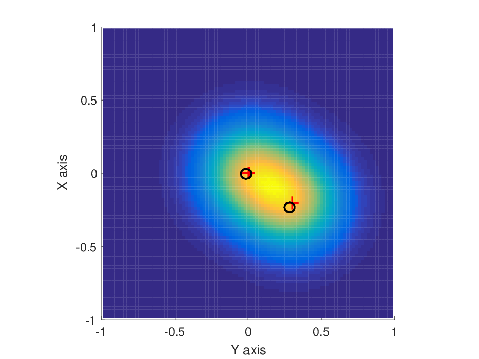
Figure 3: Localizing two sources using M=200M=200 samples, where red crosses denote the true source locations, and black circles denote the estimates. The color map represents the aggregate power field generated by the two sources.

Fig. 2 depicts the MSE of the source location versus the number of samples MM. In the single source case,the coefficient of the worst case upper bound (11) is chosen as Cμ=1C_{\mu}=1 to demonstrate the asymptotic decay rate of the worst case squared error bound. The decay rate of the analytic worst case error bound is roughly the same as the MSE obtained from the numerical experiment. It is expected that as MM increases, the two curves merge in an asymptotic way. As a benchmark, the proposed scheme requires less than half of the samples to achieve similar performance to that of the naive baseline even for small MM (around 5050). More importantly, it demonstrates a higher MSE decay rate, where for medium MM (around 200200), the proposed scheme reduces the number of samples to 1/101/10. In the double source case, there is an error floor for the naive scheme, because the location that observes the highest power may not be either one of the source locations. As a comparison, there is no error floor in for proposed scheme as MM increases.

Fig. 3 shows an example on simultaneously localizing two sources (red crosses). Although the aggregate power field has only one peak, the algorithm (black circles) is able to separate the two sources.

VI Conclusions

This paper developed source localization algorithms from a few power measurement samples, while no specific energy-decay model is assumed. Instead, the proposed method only exploited the structural property of the power field generated by the sources. Analytical results were developed to demonstrate that the proposed algorithm decreases the localization error at a higher rate than the baseline algorithm when the number of samples increases. In addition, a rotated eigenstructure analysis technique was derived for simultaneously localizing two sources. Numerical results demonstrate the performance advantage in localizing single or double sources.

Acknowledgments

This research was supported, in part, by National Science Foundation under Grant NSF CNS-1213128, CCF-1410009, CPS-1446901, Grant ONR N00014-15-1-2550, and Grant AFOSR FA9550-12-1-0215.

Appendix

VI-A Proof of Lemma 1

τ′(t)\displaystyle\tau^{{}^{\prime}}(t) =dd​t​∫−∞∞u⁡(x)​u​(x−t)​𝑑x\displaystyle=\frac{d}{dt}\int_{-\infty}^{\infty}u(x)u(x-t)dx
=∫−∞∞−u(x)u′(x−t)dx\displaystyle=\int_{-\infty}^{\infty}-u(x)u^{{}^{\prime}}(x-t)dx
=−∫−∞0u(z+t)u′(z)dz−∫0∞u(z+t)u′(z)dz\displaystyle=-\int_{-\infty}^{0}u(z+t)u^{{}^{\prime}}(z)dz-\int_{0}^{\infty}u(z+t)u^{{}^{\prime}}(z)dz
=−∫−∞0u(z+t)u′(z)dz+∫0∞u(z+t)u′(−z)dz\displaystyle=-\int_{-\infty}^{0}u(z+t)u^{{}^{\prime}}(z)dz+\int_{0}^{\infty}u(z+t)u^{{}^{\prime}}(-z)dz (18)
=−∫−∞0u(z+t)u′(z)dz+∫−∞0u(−w+t)u′(w)dw\displaystyle=-\int_{-\infty}^{0}u(z+t)u^{{}^{\prime}}(z)dz+\int_{-\infty}^{0}u(-w+t)u^{{}^{\prime}}(w)dw (19)
=−∫−∞0[u(z+t)−u(−z+t)]u′(z)dz\displaystyle=-\int_{-\infty}^{0}\big[u(z+t)-u(-z+t)\big]u^{{}^{\prime}}(z)dz
=−∫−∞0[u(z+t)−u(z−t)]u′(z)dz\displaystyle=-\int_{-\infty}^{0}\big[u(z+t)-u(z-t)\big]u^{{}^{\prime}}(z)dz (20)
<0\displaystyle<0

where (18) is due to the change of variable z=x−tz=x-t and u′(z)=−u′(−z)u^{{}^{\prime}}(z)=-u^{{}^{\prime}}(-z), (19) is to change the variable z=−wz=-w, (20) exploits the fact that u⁡(x)=u⁡(−x)u(x)=u(-x), and the last inequality is due to u⁡(z+t)−u⁡(z−t)>0u(z+t)-u(z-t)>0 and u′(z)>0u^{{}^{\prime}}(z)>0 for all z<0z<0.

VI-B Proof of Theorem 1

To simplify the algebra, we only focus on the dominant terms w.r.t. ncn_{c} as ncn_{c} goes large.

VI-B1 Upper Bound of the Sampling Error

For notational convenience, define u1​(x)=u⁡(x−x1S)u_{1}(x)=u(x-x_{1}^{\text{S}}) and v1​(y)=u⁡(x−y1S)v_{1}(y)=u(x-y_{1}^{\text{S}}). Consider the sampling position (x,y)∈𝒢i​j(x,y)\in\mathcal{G}_{ij}. Using a Taylor expansion, we have

|h1​(x,y)−h1​(x1,y1)|\displaystyle|h_{1}(x,y)-h_{1}(x_{1},y_{1})|
=α​|u1​(x)​v1​(y)−u1​(x1)​v1​(y1)|\displaystyle\quad=\alpha|u_{1}(x)v_{1}(y)-u_{1}(x_{1})v_{1}(y_{1})|
=α|(u1(x1)+u1′(x1)(x−x1))\displaystyle\quad=\alpha\big|\big(u_{1}(x_{1})+u_{1}^{{}^{\prime}}(x_{1})(x-x_{1})\big)
×(v1(y1)+v1′(y1)(y−y1))−u1(x1)v1(y1)\displaystyle\qquad\qquad\times\big(v_{1}(y_{1})+v_{1}^{{}^{\prime}}(y_{1})(y-y_{1})\big)-u_{1}(x_{1})v_{1}(y_{1})
+o(x−x1)+o(y−y1)|\displaystyle\qquad\qquad\qquad\qquad\qquad\qquad+o(x-x_{1})+o(y-y_{1})\big|
=α|u1(x1)v1′(y1)(y−y1)+v1(y1)u1′(x1)(x−x1)|\displaystyle=\alpha\big|u_{1}(x_{1})v_{1}^{{}^{\prime}}(y_{1})(y-y_{1})+v_{1}(y_{1})u_{1}^{{}^{\prime}}(x_{1})(x-x_{1})\big|
+o⁡(x−x1)+o⁡(y−y1)\displaystyle\qquad\qquad\qquad\qquad\qquad\qquad+o(x-x_{1})+o(y-y_{1})
≤α​u​(0)​Ku​Lnc+o⁡(Lnc)\displaystyle\leq\alpha u(0)K_{u}\frac{L}{n_{c}}+o\Big(\frac{L}{n_{c}}\Big)

from the property u⁡(x)≤u⁡(0)u(x)\leq u(0) and |u′(x)|≤Ku|u^{{}^{\prime}}(x)|\leq K_{u}.

From (2), we have

|H^i​j−Hi​j|\displaystyle|\hat{H}_{ij}-H_{ij}| =(Lnc)2​|h1​(x,y)−h1​(x1,y1)|\displaystyle=\bigg(\frac{L}{n_{c}}\bigg)^{2}|h_{1}(x,y)-h_{1}(x_{1},y_{1})|
≤α​u​(0)​Ku​L3nc3+o⁡(L3nc3).\displaystyle\leq\alpha u(0)K_{u}\frac{L^{3}}{n_{c}^{3}}+o\Big(\frac{L^{3}}{n_{c}^{3}}\Big). (21)

As a result,

‖𝒫Ω​(𝐇^c−𝐇)‖F2\displaystyle\|\mathcal{P}_{\Omega}(\hat{\mathbf{H}}_{\text{c}}-\mathbf{H})\|_{\text{F}}^{2} =∑(i,j)∈Ω|H^i​j−Hi​j|2\displaystyle=\sum_{(i,j)\in\Omega}|\hat{H}_{ij}-H_{ij}|^{2}
≤M​(α​u​(0)​Ku​L3/nc3)2≜ϵ¯2.\displaystyle\leq M\left(\alpha u(0)K_{u}L^{3}/n_{c}^{3}\right)^{2}\triangleq\bar{\epsilon}^{2}.

VI-B2 Matrix Completion with Noise and Singular Vector Perturbation

When there is sampling noise, the performance of matrix completion can be evaluated by the following result.

Lemma 2 (Matrix completion with noise [13]).

Consider that ϵ\epsilon in (5) is chosen such that ‖𝒫Ω​(𝐇^−𝐇)‖F≤ϵ=ϵ¯\|\mathcal{P}_{\Omega}(\hat{\mathbf{H}}-\mathbf{H})\|_{\text{F}}\leq\epsilon=\bar{\epsilon}. Then, with high probability,

δ≜‖𝐇^c−𝐇‖F≤4​(2+p)​ncp​ϵ¯+2​ϵ¯\delta\triangleq\|\hat{\mathbf{H}}_{\text{c}}-\mathbf{H}\|_{\text{F}}\leq 4\sqrt{\frac{(2+p)n_{c}}{p}}\bar{\epsilon}+2\bar{\epsilon} (22)

where p=M/nc2p=M/n_{c}^{2}.

As we focus on not too small ncn_{c}, which is chosen to be such that M≈C​nc​(log⁡nc)2M\approx Cn_{c}(\log n_{c})^{2}, the bound (22) can be simplified as

δ\displaystyle\delta ≤4​(2+C​nc​(log⁡nc)2/nc2)​ncC​nc​(log⁡nc)2/nc2​ϵ+2​ϵ\displaystyle\leq 4\sqrt{\frac{(2+Cn_{c}(\log n_{c})^{2}/n_{c}^{2})n_{c}}{Cn_{c}(\log n_{c})^{2}/n_{c}^{2}}}\epsilon+2\epsilon
≈32C​nclog⁡nc​ϵ.\displaystyle\approx\sqrt{\frac{32}{C}}\frac{n_{c}}{\log n_{c}}\epsilon.

Let 𝐮1\mathbf{u}_{1} and 𝐮^1=𝐮1+𝐞1\hat{\mathbf{u}}_{1}=\mathbf{u}_{1}+\mathbf{e}_{1} be the dominant left singular vectors of 𝐇\mathbf{H} and 𝐇^c\hat{\mathbf{H}}_{c}, respectively. We exploit the following classical result from singular vector perturbation analysis.

Lemma 3 (Singular vector perturbation [15]).

Let σ1\sigma_{1} and σ2\sigma_{2} be the first and second dominant singular values of 𝐇\mathbf{H}. Then,

sin⁡∠⁡(𝐮1,𝐮^1)≤2​‖𝐇^c−𝐇‖Fσ1−σ2=2​δσ1−σ2.\sin\angle(\mathbf{u}_{1},\hat{\mathbf{u}}_{1})\leq\frac{2\|\hat{\mathbf{H}}_{\text{c}}-\mathbf{H}\|_{\text{F}}}{\sigma_{1}-\sigma_{2}}=\frac{2\delta}{\sigma_{1}-\sigma_{2}}.

By exploiting Lemma 3 for our case, we have

sin⁡∠⁡(𝐮1,𝐮^1)\displaystyle\sin\angle(\mathbf{u}_{1},\hat{\mathbf{u}}_{1}) =1−|𝐮1T​(𝐮1+𝐞1)|2\displaystyle=\sqrt{1-\big|\mathbf{u}_{1}^{\text{T}}(\mathbf{u}_{1}+\mathbf{e}_{1})\big|^{2}}
=−2​𝐮1T​𝐞1+|𝐮1T​𝐞1|2\displaystyle=\sqrt{-2\mathbf{u}_{1}^{\text{T}}\mathbf{e}_{1}+\big|\mathbf{u}_{1}^{\text{T}}\mathbf{e}_{1}\big|^{2}}
≈2​|𝐮1T​𝐞1|\displaystyle\approx\sqrt{2\big|\mathbf{u}_{1}^{\text{T}}\mathbf{e}_{1}\big|}

where |⋅||\cdot| denotes the absolute value operator, and we drop the second order term |𝐮1T​𝐞1|2|\mathbf{u}_{1}^{\text{T}}\mathbf{e}_{1}|^{2}, since |𝐮1T​𝐞1||\mathbf{u}_{1}^{\text{T}}\mathbf{e}_{1}| is small as we focus on large nc​(M)n_{c}(M). We also note that 𝐮1T​𝐞1≤0\mathbf{u}_{1}^{\text{T}}\mathbf{e}_{1}\leq 0.

Consider that we have chosen M≈C​nc​(log⁡nc)2M\approx Cn_{c}(\log n_{c})^{2}, and moreover, 𝐇\mathbf{H} is a rank-1 matrix with singular value σ1=α\sigma_{1}=\alpha. As a result,

2​|𝐮1T​𝐞1|≈sin2⁡∠⁡(𝐮1,𝐮^1)≤(2​δα)2\displaystyle 2\big|\mathbf{u}_{1}^{\text{T}}\mathbf{e}_{1}\big|\approx\sin^{2}\angle(\mathbf{u}_{1},\hat{\mathbf{u}}_{1})\leq\Big(\frac{2\delta}{\alpha}\Big)^{2} ≤4α2​32C​(nclog⁡nc)2​ϵ¯2\displaystyle\leq\frac{4}{\alpha^{2}}\frac{32}{C}\Big(\frac{n_{c}}{\log n_{c}}\Big)^{2}\bar{\epsilon}^{2}
=128​u​(0)2​Ku2​L6​nc−3.\displaystyle=128u(0)^{2}K_{u}^{2}L^{6}n_{c}^{-3}.

VI-B3 Estimator based on Reflected Correlation

Let e⁡(x)=u^​(x)−u1​(x)e(x)=\hat{u}(x)-u_{1}(x). Define a reflected correlation function as

R⁡(t,x1S)=∫−∞∞u⁡(x−x1S)​u​(−x−x1S+t)​𝑑x.R(t;x_{1}^{\text{S}})=\int_{-\infty}^{\infty}u(x-x_{1}^{\text{S}})u(-x-x_{1}^{\text{S}}+t)dx.

Then, it follows that R⁡(t,x1S)=τ⁡(2​x1S−t)R(t;x_{1}^{\text{S}})=\tau(2x_{1}^{\text{S}}-t). As a result, we have

R^​(t,𝐮^1)\displaystyle\hat{R}(t;\hat{\mathbf{u}}_{1})
=∫−∞∞(u1​(x)+e⁡(x))​(u1​(−x+t)+e⁡(−x+t))​𝑑x\displaystyle\quad=\int_{-\infty}^{\infty}\Big(u_{1}(x)+e(x)\Big)\Big(u_{1}(-x+t)+e(-x+t)\Big)dx
=∫−∞∞u1​(x)​u1​(−x+t)​𝑑x+∫−∞∞u1​(x)​e​(−x+t)​𝑑x\displaystyle\quad=\int_{-\infty}^{\infty}u_{1}(x)u_{1}(-x+t)dx+\int_{-\infty}^{\infty}u_{1}(x)e(-x+t)dx
∫−∞∞e⁡(x)​u1​(−x+t)​𝑑x+∫−∞∞e⁡(x)​e​(−x+t)​𝑑x\displaystyle\qquad\qquad\int_{-\infty}^{\infty}e(x)u_{1}(-x+t)dx+\int_{-\infty}^{\infty}e(x)e(-x+t)dx
≈R⁡(t,x1S)+∫−∞∞u1​(x)​e​(−x+t)​𝑑x\displaystyle\quad\approx R(t;x_{1}^{\text{S}})+\int_{-\infty}^{\infty}u_{1}(x)e(-x+t)dx
+∫+∞−∞e(−y+t)u1(y)(−dy)\displaystyle\qquad\qquad\qquad+\int_{+\infty}^{-\infty}e(-y+t)u_{1}(y)(-dy) (23)
=R⁡(t,x1S)+2​∫−∞∞u1​(x)​e​(−x+t)​𝑑x\displaystyle\quad=R(t;x_{1}^{\text{S}})+2\int_{-\infty}^{\infty}u_{1}(x)e(-x+t)dx
≈R⁡(t,x1S)+2​𝐮1T​𝐞1−t\displaystyle\quad\approx R(t;x_{1}^{\text{S}})+2\mathbf{u}_{1}^{\text{T}}\mathbf{e}_{1}^{-t} (24)

where the first approximation (23) is by dropping the second order term ∫−∞∞e⁡(x)​e​(−x+t)​𝑑x\int_{-\infty}^{\infty}e(x)e(-x+t)dx, and the second approximation (24) is to use the inner product 𝐮1T​𝐞1−t\mathbf{u}_{1}^{\text{T}}\mathbf{e}_{1}^{-t} to approximate the integral based on assumptions A1 and A2 in Section III. As a result, we have R⁡(t,x1S)−R^​(t,𝐮^1)≈−2​𝐮1T​𝐞1−tR(t;x_{1}^{\text{S}})-\hat{R}(t;\hat{\mathbf{u}}_{1})\approx-2\mathbf{u}_{1}^{\text{T}}\mathbf{e}_{1}^{-t}.

Recall that t^=2​x^1S\hat{t}=2\hat{x}_{1}^{\text{S}} maximizes R^​(t^,𝐮^1)\hat{R}(\hat{t};\hat{\mathbf{u}}_{1}) and t∗=2​x1St^{*}=2x_{1}^{\text{S}} maximizes R⁡(t∗,x1S)=τ⁡(2​x1S−t∗)R(t^{*};x_{1}^{\text{S}})=\tau(2x_{1}^{\text{S}}-t^{*}). We have

τ⁡(0)−τ⁡(2​|x^1S−x1S|)\displaystyle\tau(0)-\tau\big(2\big|\hat{x}_{1}^{\text{S}}-x_{1}^{\text{S}}\big|\big)
=R⁡(t∗,x1S)−R^​(t^,𝐮^1)\displaystyle\qquad=R(t^{*};x_{1}^{\text{S}})-\hat{R}(\hat{t};\hat{\mathbf{u}}_{1})
≈−2​𝐮1T​𝐞1−t\displaystyle\qquad\approx-2\mathbf{u}_{1}^{\text{T}}\mathbf{e}_{1}^{-t}
≤Ce​2​|𝐮1T​𝐞1|\displaystyle\qquad\leq C_{e}2\big|\mathbf{u}_{1}^{\text{T}}\mathbf{e}_{1}\big|
≤μu​L6​n−3+o⁡(nc−3)\displaystyle\qquad\leq\mu_{u}L^{6}n^{-3}+o(n_{c}^{-3})

where μu=Ce​128​u​(0)2​Ku2\mu_{u}=C_{e}128u(0)^{2}K_{u}^{2} and o⁡(nc−3)o(n_{c}^{-3}) is due to the fact that we keep omitting the higher order terms. Finally, we obtain

τ⁡(2​|x^1S−x1S|)=1−μu​L6​n−3+o⁡(nc−3)\tau\big(2\big|\hat{x}_{1}^{\text{S}}-x_{1}^{\text{S}}\big|\big)=1-\mu_{u}L^{6}n^{-3}+o(n_{c}^{-3})

and hence,

|x^1S−x1S|≤12​τ−1​(1−μu​L6​nc−3+o⁡(nc−3)).\big|\hat{x}_{1}^{\text{S}}-x_{1}^{\text{S}}\big|\leq\frac{1}{2}\tau^{-1}(1-\mu_{u}L^{6}n_{c}^{-3}+o(n_{c}^{-3})).

VI-C Proof of Theorem 2

We first study the singular vectors in double source case.

Lemma 4 (Singular vectors in two source case).

Let 𝐮k​(θ)\mathbf{u}_{k}(\theta) and 𝐯k​(θ)\mathbf{v}_{k}(\theta) be the vectors defined following (3) and (4) in the rotated coordinate system 𝒞θ\mathcal{C}_{\theta}. The SVD of 𝐇θ\mathbf{H}_{\theta} is given by

𝐇θ=α1​𝐩1​𝐪1T+α2​𝐩2​𝐪2T\mathbf{H}_{\theta}=\alpha_{1}\mathbf{p}_{1}\mathbf{q}_{1}^{\text{T}}+\alpha_{2}\mathbf{p}_{2}\mathbf{q}_{2}^{\text{T}} (25)

where α1=α2​‖𝐮1+𝐮2‖​‖𝐯1+𝐯2‖\alpha_{1}=\frac{\alpha}{2}\|\mathbf{u}_{1}+\mathbf{u}_{2}\|\|\mathbf{v}_{1}+\mathbf{v}_{2}\| and α2=α2​‖𝐮1−𝐮2‖​‖𝐯1−𝐯2‖\alpha_{2}=\frac{\alpha}{2}\|\mathbf{u}_{1}-\mathbf{u}_{2}\|\|\mathbf{v}_{1}-\mathbf{v}_{2}\| are the singular values, and

𝐩1=𝐮1+𝐮2‖𝐮1+𝐮2‖,𝐪1=𝐯1+𝐯2‖𝐯1+𝐯2‖\mathbf{p}_{1}=\frac{\mathbf{u}_{1}+\mathbf{u}_{2}}{\|\mathbf{u}_{1}+\mathbf{u}_{2}\|},\quad\mathbf{q}_{1}=\frac{\mathbf{v}_{1}+\mathbf{v}_{2}}{\|\mathbf{v}_{1}+\mathbf{v}_{2}\|}
𝐩2=𝐮1−𝐮2‖𝐮1−𝐮2‖,𝐪2=𝐯1−𝐯2‖𝐯1−𝐯2‖\mathbf{p}_{2}=\frac{\mathbf{u}_{1}-\mathbf{u}_{2}}{\|\mathbf{u}_{1}-\mathbf{u}_{2}\|},\quad\mathbf{q}_{2}=\frac{\mathbf{v}_{1}-\mathbf{v}_{2}}{\|\mathbf{v}_{1}-\mathbf{v}_{2}\|}

are the corresponding singular vectors.

Proof.

First,

𝐇θ\displaystyle\mathbf{H}_{\theta} =α¯​(𝐮1​𝐯1T+𝐮2​𝐯2T)\displaystyle=\bar{\alpha}\big(\mathbf{u}_{1}\mathbf{v}_{1}^{\text{T}}+\mathbf{u}_{2}\mathbf{v}_{2}^{\text{T}}\big)
=α¯2​[(𝐮1+𝐮2)​(𝐯1+𝐯2)T+(𝐮1−𝐮2)​(𝐯1−𝐯2)T]\displaystyle=\frac{\bar{\alpha}}{2}\Big[(\mathbf{u}_{1}+\mathbf{u}_{2})(\mathbf{v}_{1}+\mathbf{v}_{2})^{\text{T}}+(\mathbf{u}_{1}-\mathbf{u}_{2})(\mathbf{v}_{1}-\mathbf{v}_{2})^{\text{T}}\Big]
=α1​𝐩1​𝐪1T+α2​𝐩2​𝐪2T\displaystyle=\alpha_{1}\mathbf{p}_{1}\mathbf{q}_{1}^{\text{T}}+\alpha_{2}\mathbf{p}_{2}\mathbf{q}_{2}^{\text{T}}

Hence, these four vectors form a decomposition of 𝐇θ\mathbf{H}_{\theta}.

Second, we have

𝐩1T​𝐩2\displaystyle\mathbf{p}_{1}^{\text{T}}\mathbf{p}_{2} =c​(𝐮1+𝐮2)T​(𝐮1−𝐮2)\displaystyle=c(\mathbf{u}_{1}+\mathbf{u}_{2})^{\text{T}}(\mathbf{u}_{1}-\mathbf{u}_{2})
=c⁡(‖𝐮1‖2−‖𝐮2‖2)\displaystyle=c\big(\|\mathbf{u}_{1}\|^{2}-\|\mathbf{u}_{2}\|^{2}\big)
=0\displaystyle=0

where c=1/(‖𝐮1+𝐮2‖​‖𝐮1−𝐮2‖)c=1/(\|\mathbf{u}_{1}+\mathbf{u}_{2}\|\|\mathbf{u}_{1}-\mathbf{u}_{2}\|). Similarly, 𝐪1T​𝐪2=0\mathbf{q}_{1}^{\text{T}}\mathbf{q}_{2}=0. In addition, all the four vectors have unit norm.

As a result, (25) is the SVD of 𝐇θ\mathbf{H}_{\theta}. ∎

Consider an arbitrary coordinate system. W.l.o.g. (due to Assumption 1), assume that the first source is located at the origin, x1S=0x_{1}^{\text{S}}=0 and y1S=0y_{1}^{\text{S}}=0, and the second source is away from the first source with distance DD and angle θ\theta to the xx-axis, x2S=D​cos⁡θx_{2}^{\text{S}}=D\cos\theta and y2S=D​sin⁡θy_{2}^{\text{S}}=D\sin\theta. In addition, defining

uc​(x,θ)≜u⁡(x−D​cos⁡θ),us​(x,θ)≜u⁡(x−D​sin⁡θ)u_{\text{c}}(x,\theta)\triangleq u(x-D\cos\theta),\qquad u_{\text{s}}(x,\theta)\triangleq u(x-D\sin\theta)

we have

𝐮1\displaystyle\mathbf{u}_{1} =δ​[u⁡(x1),u⁡(x2),…,u⁡(xN)]T\displaystyle=\sqrt{\delta}\big[u(x_{1}),u(x_{2}),\dots,u(x_{N})\big]^{\text{T}}
𝐯1\displaystyle\mathbf{v}_{1} =δ​[u⁡(y1),u⁡(y2),…,u⁡(yM)]T\displaystyle=\sqrt{\delta}\big[u(y_{1}),u(y_{2}),\dots,u(y_{M})\big]^{\text{T}}
𝐮2\displaystyle\mathbf{u}_{2} =δ​[uc​(x1,θ),uc​(x2,θ),…,uc​(xN,θ)]T\displaystyle=\sqrt{\delta}\big[u_{\text{c}}(x_{1},\theta),u_{\text{c}}(x_{2},\theta),\dots,u_{\text{c}}(x_{N},\theta)\big]^{\text{T}}
𝐯2\displaystyle\mathbf{v}_{2} =δ​[us​(y1,θ),us​(y2,θ),…,us​(yM,θ)]T.\displaystyle=\sqrt{\delta}\big[u_{\text{s}}(y_{1},\theta),u_{\text{s}}(y_{2},\theta),\dots,u_{\text{s}}(y_{M},\theta)\big]^{\text{T}}.

Based on assumption A1 and A2, we have

‖𝐮k‖2=(Ln)2​∑i=1Nu​(xi−xkS)2\displaystyle\|\mathbf{u}_{k}\|^{2}=\Big(\frac{L}{n}\Big)^{2}\sum_{i=1}^{N}u(x_{i}-x_{k}^{\text{S}})^{2} ≈∫x1xn−1u​(x−xkS)2​𝑑x\displaystyle\approx\int_{x_{1}}^{x_{n-1}}u(x-x_{k}^{\text{S}})^{2}dx
≈∫−∞∞u​(x−xkS)2​𝑑x=1\displaystyle\approx\int_{-\infty}^{\infty}u(x-x_{k}^{\text{S}})^{2}dx=1 (26)

and similar integrals apply to 𝐯k\mathbf{v}_{k}.

As an equivalent statement to Theorem 2, we need to show that ρ⁡(θ)\rho(\theta) is a strictly increasing function in θ∈(0,π4)\theta\in(0,\frac{\pi}{4}). Equivalently, we should prove that the function

λ2​(𝐇θ)2λ1​(𝐇θ)2\displaystyle\frac{\lambda_{2}(\mathbf{H}_{\theta})^{2}}{\lambda_{1}(\mathbf{H}_{\theta})^{2}}
≈∫−∞∞(u⁡(x)−uc​(x,θ))2​𝑑x∫−∞∞(u⁡(x)+uc​(x,θ))2​𝑑x​∫−∞∞(u⁡(x)−us​(x,θ))2​𝑑x∫−∞∞(u⁡(x)+us​(x,θ))2​𝑑x\displaystyle\quad\approx\frac{\int_{-\infty}^{\infty}\big(u(x)-u_{\text{c}}(x,\theta)\big)^{2}dx}{\int_{-\infty}^{\infty}\big(u(x)+u_{\text{c}}(x,\theta)\big)^{2}dx}\frac{\int_{-\infty}^{\infty}\big(u(x)-u_{\text{s}}(x,\theta)\big)^{2}dx}{\int_{-\infty}^{\infty}\big(u(x)+u_{\text{s}}(x,\theta)\big)^{2}dx}
≜μ⁡(θ)\displaystyle\quad\triangleq\mu(\theta)

is strictly increasing in θ∈(0,π4)\theta\in(0,\frac{\pi}{4}), where the approximated integrals are obtained from (26).

To simplify the notation, define the integration operator ⟨⋅⟩\left\langle\cdot\right\rangle as

⟨f⟩≜∫−∞∞f⁡(x,θ)​𝑑x\left\langle f\right\rangle\triangleq\int_{-\infty}^{\infty}f(x,\theta)dx

for a function f⁡(x,θ)f(x,\theta). By definition, the integration operator is linear and satisfies the additive property, i.e., ⟨a​f⟩=a​⟨f⟩\langle af\rangle=a\langle f\rangle and ⟨f+g⟩=⟨f⟩+⟨g⟩\langle f+g\rangle=\langle f\rangle+\langle g\rangle, for a constant aa and a function g⁡(x,θ)g(x,\theta). As a result, ⟨(u−uc)2⟩=⟨u2⟩+⟨uc2⟩−2​⟨u⋅uc⟩=2​(1−⟨u⋅uc⟩)\langle(u-u_{\text{c}})^{2}\rangle=\langle u^{2}\rangle+\langle u_{\text{c}}^{2}\rangle-2\langle u\cdot u_{\text{c}}\rangle=2\big(1-\langle u\cdot u_{\text{c}}\rangle\big), and the function μ⁡(θ)\mu(\theta) can be written as

μ⁡(θ)=(1−⟨u⋅uc⟩)​(1−⟨u⋅us⟩)(1+⟨u⋅uc⟩)​(1+⟨u⋅us⟩).\mu(\theta)=\frac{\big(1-\langle u\cdot u_{\text{c}}\rangle\big)\big(1-\langle u\cdot u_{\text{s}}\rangle\big)}{\big(1+\langle u\cdot u_{\text{c}}\rangle\big)\big(1+\langle u\cdot u_{\text{s}}\rangle\big)}. (27)

In addition, from the properties in calculus, if f⁡(x,θ)f(x,\theta) and ∂∂θ​f​(x,θ)\frac{\partial}{\partial\theta}f(x,\theta) are continuous in θ,\theta, then

dd​θ​⟨f⟩\displaystyle\frac{d}{d\theta}\left\langle f\right\rangle =dd​θ​∫−∞∞f⁡(x,θ)​𝑑x\displaystyle=\frac{d}{d\theta}\int_{-\infty}^{\infty}f(x,\theta)dx
=∫−∞∞∂∂θ​f​(x,θ)​𝑑x=⟨∂∂θ​f⟩.\displaystyle=\int_{-\infty}^{\infty}\frac{\partial}{\partial\theta}f(x,\theta)dx=\Big\langle\frac{\partial}{\partial\theta}f\Big\rangle.

Therefore, defining

uc′(x,θ)\displaystyle u_{\text{c}}^{{}^{\prime}}(x,\theta) ≜dd​x​u​(x)|x=x−D​cos⁡θ\displaystyle\triangleq\frac{d}{dx}u(x)\big|_{x=x-D\cos\theta}
us′(x,θ)\displaystyle u_{\text{s}}^{{}^{\prime}}(x,\theta) ≜dd​x​u​(x)|x=x−D​sin⁡θ\displaystyle\triangleq\frac{d}{dx}u(x)\big|_{x=x-D\sin\theta}

we have

dd​θ​⟨u⋅uc⟩\displaystyle\frac{d}{d\theta}\langle u\cdot u_{\text{c}}\rangle =⟨u⋅∂∂θuc(x,θ)⟩=⟨u⋅uc′⟩Dsinθ\displaystyle=\langle u\cdot\frac{\partial}{\partial\theta}u_{\text{c}}(x,\theta)\rangle=\langle u\cdot u_{\text{c}}^{{}^{\prime}}\rangle D\sin\theta
dd​θ​⟨u⋅us⟩\displaystyle\frac{d}{d\theta}\langle u\cdot u_{\text{s}}\rangle =⟨u⋅∂∂θus(x,θ)⟩=−⟨u⋅us′⟩Dcosθ.\displaystyle=\langle u\cdot\frac{\partial}{\partial\theta}u_{\text{s}}(x,\theta)\rangle=-\langle u\cdot u_{\text{s}}^{{}^{\prime}}\rangle D\cos\theta.

With some algebra, the derivative of μ⁡(θ)\mu(\theta) can be obtained as

dd​θ​μ​(θ)\displaystyle\frac{d}{d\theta}\mu(\theta) =η[Dcosθ⟨u⋅us′⟩(1−⟨u⋅uc⟩2)\displaystyle=\eta\Big[D\cos\theta\langle u\cdot u_{\text{s}}^{{}^{\prime}}\rangle\big(1-\langle u\cdot u_{\text{c}}\rangle^{2}\big)
−Dsinθ⟨u⋅uc′⟩(1−⟨u⋅us⟩2)]\displaystyle\qquad\qquad-D\sin\theta\langle u\cdot u_{\text{c}}^{{}^{\prime}}\rangle\big(1-\langle u\cdot u_{\text{s}}\rangle^{2}\big)\Big]
=η[−t⋅τ′(s)(1−τ(t)2)+s⋅τ′(t)(1−τ(s)2)]\displaystyle=\eta\Big[-t\cdot\tau^{{}^{\prime}}(s)\big(1-\tau(t)^{2}\big)+s\cdot\tau^{{}^{\prime}}(t)\big(1-\tau(s)^{2}\big)\Big]

where η=2​(1+⟨u⋅uc⟩)−2​(1+⟨u⋅us⟩)−2\eta=2\big(1+\langle u\cdot u_{\text{c}}\rangle\big)^{-2}\big(1+\langle u\cdot u_{\text{s}}\rangle\big)^{-2}, t=D​cos⁡θt=D\cos\theta, and s=D​sin⁡θs=D\sin\theta.

Note that 0<s<t0<s<t for 0<θ<π40<\theta<\frac{\pi}{4}. Applying condition (14), we have

dd​θ​μ​(θ)\displaystyle\frac{d}{d\theta}\mu(\theta) >η⋅t⋅τ′(s)[(1−τ(s)2)−(1−τ(t)2)]\displaystyle>\eta\cdot t\cdot\tau^{{}^{\prime}}(s)\Big[\big(1-\tau(s)^{2}\big)-\big(1-\tau(t)^{2}\big)\Big]
=η⋅t⋅τ′(s)(τ(t)2−τ(s)2)\displaystyle=\eta\cdot t\cdot\tau^{{}^{\prime}}(s)\big(\tau(t)^{2}-\tau(s)^{2}\big)
>0\displaystyle>0

since τ′(s)<0\tau^{{}^{\prime}}(s)<0 and τ⁡(t)<τ⁡(s)\tau(t)<\tau(s) for 0<s<t0<s<t.

This confirms that μ⁡(θ)\mu(\theta) is a strictly increasing function, and hence ρ⁡(θ)\rho(\theta) is a strictly increasing function in θ∈(0,π4)\theta\in(0,\frac{\pi}{4}). The results in Theorem 2 is confirmed.

References

  • [1] A. Beck, P. Stoica, and J. Li, “Exact and approximate solutions of source localization problems,” IEEE Trans. Signal Process., vol. 56, no. 5, pp. 1770–1778, 2008.
  • [2] H.-D. Qi, N. Xiu, and X. Yuan, “A lagrangian dual approach to the single-source localization problem,” IEEE Trans. Signal Process., vol. 61, no. 15, pp. 3815–3826, 2013.
  • [3] X. Sheng and Y.-H. Hu, “Maximum likelihood multiple-source localization using acoustic energy measurements with wireless sensor networks,” IEEE Trans. Signal Process., vol. 53, no. 1, pp. 44–53, 2005.
  • [4] C. Meesookho, U. Mitra, and S. Narayanan, “On energy-based acoustic source localization for sensor networks,” IEEE Trans. Signal Process., vol. 56, no. 1, pp. 365–377, 2008.
  • [5] Y. Liu, Y. H. Hu, and Q. Pan, “Distributed, robust acoustic source localization in a wireless sensor network,” IEEE Trans. Signal Process., vol. 60, no. 8, pp. 4350–4359, 2012.
  • [6] I. Ziskind and M. Wax, “Maximum likelihood localization of multiple sources by alternating projection,” Proc. IEEE Int. Conf. Acoustics, Speech, and Signal Processing, vol. 36, no. 10, pp. 1553–1560, 1988.
  • [7] R. Lefort, G. Real, and A. Drémeau, “Direct regressions for underwater acoustic source localization in fluctuating oceans,” Applied Acoustics, vol. 116, pp. 303–310, 2017.
  • [8] X. Nguyen, M. I. Jordan, and B. Sinopoli, “A kernel-based learning approach to ad hoc sensor network localization,” ACM Trans. on Sensor Networks, vol. 1, no. 1, pp. 134–152, 2005.
  • [9] Y. Jin, W.-S. Soh, and W.-C. Wong, “Indoor localization with channel impulse response based fingerprint and nonparametric regression,” IEEE Trans. Wireless Commun., vol. 9, no. 3, pp. 1120–1127, 2010.
  • [10] W. Kim, J. Park, J. Yoo, H. J. Kim, and C. G. Park, “Target localization using ensemble support vector regression in wireless sensor networks,” IEEE Trans. on Cybernetics, vol. 43, no. 4, pp. 1189–1198, 2013.
  • [11] S. Choudhary and U. Mitra, “Analysis of target detection via matrix completion,” in Proc. IEEE Int. Conf. Acoustics, Speech, and Signal Processing, 2015, pp. 3771–3775.
  • [12] S. Choudhary, N. Kumar, S. Narayanan, and U. Mitra, “Active target localization using low-rank matrix completion and unimodal regression,” arXiv preprint arXiv:1601.07254, 2016.
  • [13] E. J. Candes and Y. Plan, “Matrix completion with noise,” Proceedings of the IEEE, vol. 98, no. 6, pp. 925–936, 2010.
  • [14] R. Peterson, R. Ziemer, and D. Borth, Introduction to spread spectrum systems. Englewood Cliffs, NJ: Prentice-Hall, 1995.
  • [15] V. Vu, “Singular vectors under random perturbation,” Random Structures & Algorithms, vol. 39, no. 4, pp. 526–538, 2011.