Information Theoretic Limits for Linear Prediction with Graph-Structured Sparsity
Abstract
We analyze the necessary number of samples for sparse vector recovery in a noisy linear prediction setup. This model includes problems such as linear regression and classification. We focus on structured graph models. In particular, we prove that sufficient number of samples for the weighted graph model proposed by Hegde and others [2] is also necessary. We use the Fano’s inequality [11] on well constructed ensembles as our main tool in establishing information theoretic lower bounds.
Keywords:
Compressive sensing, Linear Prediction, Classification, Fano’s Inequality, Mutual Information, Kullback Leibler divergence.
1 Introduction
Sparse vectors are widely used tools in fields related to high dimensional data analytics such as machine learning, compressed sensing and statistics. This makes estimation of sparse vectors an important field of research. In a compressive sensing setting, the problem is to closely approximate a dimensional signal by an sparse vector without losing much information. For regression, this is usually done by observing the inner product of the signal with a design matrix. It is a well known fact that if the design matrix satisfies the Restricted Isometry Property (RIP) then estimation can be done efficiently with a sample complexity of . Many algorithms such as CoSamp [5], Subspace Pursuit (SP) [4] and Iterative Hard Thresholding (IHT) [3] provide high probability performance guarantees. Baraniuk and others [1] came up with a model based sparse recovery framework. Under this framework, the sufficient number of samples for correct recovery is logarithmic with respect to the cardinality of the sparsity model.
A major issue with the model based framework is that it does not provide any recovery algorithm on its own. In fact, it is some times very hard to come up with an efficient recovery algorithm. Addressing this issue, Hegde and others [2] came up with a weighted graph model for graph structured sparsity and provided a nearly linear time recovery algorithm. They also analyzed the sufficient number of samples for efficient recovery. In this paper, we will provide the necessary condition on the sample complexity for sparse recovery on a weighted graph model. We will also note that our information theoretic lower bound can be applied not only to linear regression but also to other linear prediction tasks such as classification.
2 Linear Prediction Model
In this section, we introduce the observation model for linear prediction and later specify how to use it for specific problems such as linear regression and classification. Formally, the problem is to estimate an sparse vector from noisy observations of the form,
| (1) |
where is the observed output, is the design matrix , is a noise vector and is a fixed function. Our task is to recover from the observations .
2.1 Linear Regression
Linear regression is a special case of the above by choosing . Then we simply have,
| (2) |
Prior work analyzes the sample complexity of sparse recovery for the linear regression setup. In particular, if the design matrix satisfies the Restricted Isometry Property (RIP) then algorithms such as CoSamp [5], Subspace Pursuit (SP) [4] and Iterative Hard Thresholding (IHT) [3] can recover quite efficiently and in a stable way with a sample complexity of . Furthermore, it is known that Gaussian random matrices (or sub-Gaussian in general) satisfy RIP [6]. If we choose our design matrix to be a Gaussian matrix and we have a good sparsity model that incorporates extra information on the sparsity structure then we can reduce the sample complexity to where is number of possible supports in the sparsity model, i.e., the cardinality of the sparsity model [1]. In the same line of work, Hegde and others [2] proposed a weighted graph based sparsity model to efficiently learn .
2.2 Classification
We can model binary classification problems by choosing or in other words, we can have,
| (3) |
Similar to the linear regression setup, there is also prior work [9], [12], [10], on analyzing the sample complexity of sparse recovery for binary classification problem (also known as 1-bit compressed sensing).
Since arguments for establishing information theoretic lower bounds are not algorithm specific, we can extend our basic argument to the both settings mentioned above. For comparison, we will use the results by Hegde and others [2] in a linear regression setup.
3 Weighted Graph Model (WGM)
In this section, we introduce the Weighted Graph Model (WGM) and formally state the sample complexity results from [2]. The Weighted Graph Model is defined on an underlying graph whose vertices are on the coefficients of the unknown sparse vector i.e. . Moreover, the graph is weighted and thus we introduce a weight function . Borrowing some notations from [2], for a forest we denote as . denotes the weight budget, denotes the sparsity (number of non-zero coefficients) of and denotes the number of connected components in . The weight-degree of a node is the largest number of adjacent nodes connected by edges with the same weight, i.e.,
| (4) |
We define the weight-degree of , to be the maximum weight-degree of any . Next, we define the Weighted Graph Model on coefficients of as follows:
Definition 1 (Definition 1 in [2]).
The is the set of supports defined as
where is number of connected components in a forest . Authors in [2] provide the following sample complexity result for linear regression under their model:
Theorem 1 (Theorem 3 in [2]).
Let be in the . Then
| (5) |
i.i.d. Gaussian observations suffice to estimate . More precisely, let be an arbitrary noise vector from equation (2) and be an i.i.d. Gaussian matrix. Then we can efficiently find an estimate such that
| (6) |
where is a constant indepenedent of all variables above.
Notice that in the noiseless case , we recover the exact . We will prove that information-theoretically, the bound on the sample complexity is tight and thus the algorithm of [2] is statistically optimal.
4 Main Results
In this section, we will state our results for both the noiseless and the noisy case. We establish an information theoretic lower bound on linear prediction problem defined on WGM. We use Fano’s inequality [11] to prove our result by carefully constructing an ensemble, i.e., a WGM. Any algorithm which infers from this particular WGM would require a minimum number of samples. Note that the use of restricted ensembles is customary for information-theoretic lower bounds [13] [14]. It follows that in the case of linear regression, the upper bound on the sample complexity by Hegde and others [2] is indeed tight.
4.1 Noiseless Case
Here, we provide a necessary condition on the sample complexity for exact recovery in the noiseless case. More formally,
Theorem 2.
There exists a particular , and a particular set of weights for the entries in the support of such that if we draw a uniformly at random and we have a data set of i.i.d. observations as defined in equation (1) with then irrespective of the procedure we use to infer on from .
Proof sketch.
We use Fano’s inequality [11] on a carefully chosen restricted ensemble to prove our theorem. A detailed proof can be found in appendix. ∎
4.2 Noisy Case
A similar result can be stated for the noisy case. However, in this case recovery is not exact but is sufficiently close in -norm with respect to noise in the signal. Another thing to note is that in [2] inferred can come from a slightly bigger WGM model but here we actually infer from the same WGM.
Theorem 3.
There exists a particular , and a particular set of weights for the entries in the support of such that if we draw a uniformly at random and we have a data set of i.i.d. observations as defined in equation (1) with then for irrespective of the procedure we use to infer on from .
Remark 1.
Note that when and then is roughly .
Proof.
We will prove this result in three steps. First, we will carefully construct an underlying graph for the WGM. Second, we will bound mutual information between and by bounding the Kullback-Leibler (KL) divergence. Third, we will bound the size of properly defined restricted ensemble to complete our proof.
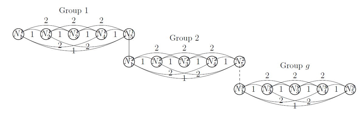

Constructing an underlying graph for the WGM
We construct an underlying graph for the WGM using the following steps:
- •
Divide nodes equally into groups with each group having nodes.
- •
For each group , we denote a node by where is the group index and is the node index. Each group , contains nodes from to .
- •
We allow for circular indexing, i.e., a node where is same as node .
- •
For each , node has an edge with nodes to with weight .
- •
Cross edges between nodes in two different groups are allowed as long as they have edge weights greater than and they do not affect .
Figure 1 shows an example of a graph constructed using the above steps. Furthermore, parameters for our satisfy the following requirements:
- R1.
,
- R2.
,
- R3.
.
These are quite mild requirements (see appendix) on the parameters and are easy to fulfill. Figure 2 shows one graph which follows our construction and also fulfills R1, R2 and R3. We define our restricted ensemble on as:
| (7) | ||||
for some and is as in Definition 1.
Our true is picked uniformly at random from the above restricted ensemble. We will prove that on this restricted ensemble, our Theorem 3 holds. We will make use of following lemmas for our proof:
Lemma 1.
Given the restricted ensemble ,
We are dealing with high dimensional cases, hence moving forward we will assume that . We state another lemma:
Lemma 2.
For some ,
Corollary 1.
Bound on the mutual information
We will assume that the elements of design matrix have been chosen at random and independently from . The linear prediction problem from Section 2 can be described by the following Markov’s chain:
| (8) |
Lets say contains i.i.d. observations of and contains i.i.d. observations of . Then using the data processing inequality [11] we can say that,
| (9) |
Hence, for our purpose it suffices to have an upper bound on . Now we can bound the mutual information by the following [8]:
| (10) |
where is the Kullback-Leibler divergence. Note that consists of i.i.d. observations of . Hence,
| (11) |
Furthermore, from equation (8) and noting that the elements of come independently from ,
We can bound the Kullback-Leibler divergence between and as follows:
The first inequality holds because , the second inequality holds by taking the largest value of numerators and the smallest value of denominators. The other inequalities follow from simple algebraic manipulation. Substituting in equation (11) we get,
| (12) |
Bound on
Now we will count elements in to complete our proof. We present the following counting argument to establish a lower bound on all the possible supports for our restricted ensemble:
- 1.
We choose one node from each of the groups in underlying graph to be root of a connected component. Each group has possible candidates for the root and hence we can choose them in possible ways.
- 2.
Since we are interested only in establishing a lower bound on , we will only consider the cases where each connected component has nodes. Moreover, given a root node in group , we will choose the remaining nodes connected with the root only from the nodes to nodes (using circular indices if needed). Construction of the graph allows us to do this. At least till the last nodes, we always include node and we never include in our selection. Furthermore, R1 guarantees that we have enough nodes to avoid any possible repetitions due to circular indices for the last nodes and R2 ensures that we have enough nodes to form a connected component. This guarantees that all the supports are unique. Hence, given a root node we have choices which across all the groups comes out to be .
- 3.
Each entry in the support of can take two values which can either be or .
It should be noted that any support chosen using the above steps satisfies constraint on weight budget, i.e., as the maximum edge weight in any connected component will always be less than or equal to . Combining all the above steps together we get:
| (13) | ||||
Using Fano’s inequality [11] and results from equation (12) and equation (13), it is easy to prove the following lemma,
Lemma 3.
If then .
5 Specific Examples
Here, we will provide counting arguments for some of the well-known sparsity structures, such as tree sparsity and block sparsity models. It should be noted that barring the count of possible supports in the specific model our technique can be used to prove lower bounds of the sample complexity for other sparsity structures.
5.1 Tree-structured sparsity model
The tree-sparsity model [1], [7] is used in many applications such as wavelet decomposition of piecewise smooth signals and images. In this model, we assume that the coefficients of the sparse signal form a ary tree and the support of the sparse signal form a rooted and connected sub-tree on nodes in this ary tree. The arrangement is such that if a node is part of this subtree then its parent is also included in it. Here, we will discuss the case of a binary tree which can be generalized to a ary tree. In particular, the following proposition provides a lower bound on the number of possible supports of an sparse signal following a binary tree-structured sparsity model.
Proposition 1.
In a binary tree-structured sparsity model , for some .
The proof of the proposition 1 follows from the fact that we have at least different choices of in our restricted ensemble. From the above and following the same proof technique as before, it is easy to prove the following corollary for the noisy case (a similar result holds for the noiseless case as well).
Corollary 2.
In a binary tree-structured sparsity model, if then .
5.2 Block sparsity model
In the block sparsity model, [1], an sparse signal, , can be represented as a matrix with rows and columns. The support of comes from columns of this matrix such that . More precisely,
Definition 2 (Definition 11 in [1]).
The above can be modeled as a graph model. In particular, we can construct a graph over all the elements in by treating nodes in the column of the matrix as connected nodes (see Fig. 3) and then our problem is to choose connected components from .
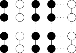
It is easy to see that the number of possible supports in this model, , would be, . Correspondingly the necessary number of samples for efficient signal recovery comes out to be . An upper bound of was derived in [1] which matches our lower bound.
6 Concluding Remarks
We proved that the necessary number of samples required to efficiently recover a sparse vector in the weighted graph model is of the same order as the sufficient number of samples provided by Hegde and others [2]. Moreover, our results not only pertain to linear regression but also apply to linear prediction problems in general.
References
- [1] R. G. Baraniuk, V. Cevher, M. F. Duarte, and C. Hegde, “Model-based compressive sensing,” IEEE Transactions on Information Theory, vol. 56, no. 4, pp. 1982–2001, 2010.
- [2] C. Hegde, P. Indyk, and L. Schmidt, “A nearly-linear time framework for graph-structured sparsity,” in Proceedings of the 32nd International Conference on Machine Learning (ICML-15), pp. 928–937, 2015.
- [3] Thomas Blumensath and Mike E Davies. Iterative hard thresholding for compressed sensing. Applied and Computational Harmonic Analysis, 27(3):265–274, 2009.
- [4] Wei Dai and Olgica Milenkovic. Subspace pursuit for compressive sensing: Closing the gap between performance and complexity. Technical report, DTIC Document, 2008.
- [5] Deanna Needell and Joel A Tropp. Cosamp: Iterative signal recovery from incomplete and inaccurate samples. Applied and Computational Harmonic Analysis, 26(3):301–321, 2009.
- [6] Richard Baraniuk, Mark Davenport, Ronald DeVore, and Michael Wakin. A simple proof of the restricted isometry property for random matrices. Constructive Approximation, 28(3):253–263, 2008.
- [7] Chinmay Hegde, Piotr Indyk, and Ludwig Schmidt. A fast approximation algorithm for tree-sparse recovery. In 2014 IEEE International Symposium on Information Theory, pages 1842–1846. IEEE, 2014.
- [8] B. Yu. Assouad, Fano, and Le Cam. In Torgersen E. Pollard D. and Yang G., editors, Festschrift for Lucien Le Cam: Research Papers in Probability and Statistics, pages 423–435. Springer New York, 1997.
- [9] Ankit Gupta, Robert D Nowak, and Benjamin Recht. Sample complexity for 1-bit compressed sensing and sparse classification. In ISIT, pages 1553–1557, 2010.
- [10] Sivakant Gopi, Praneeth Netrapalli, Prateek Jain, and Aditya V Nori. One-bit compressed sensing: Provable support and vector recovery. In ICML (3), pages 154–162, 2013.
- [11] T. Cover and J. Thomas. Elements of Information Theory. John Wiley & Sons, 2nd edition, 2006.
- [12] Albert Ai, Alex Lapanowski, Yaniv Plan, and Roman Vershynin. One-bit compressed sensing with non-gaussian measurements. Linear Algebra and its Applications, 441:222–239, 2014.
- [13] Narayana P Santhanam and Martin J Wainwright. Information-theoretic limits of selecting binary graphical models in high dimensions. IEEE Transactions on Information Theory, 58(7):4117–4134, 2012.
- [14] Wei Wang, Martin J Wainwright, and Kannan Ramchandran. Information-theoretic bounds on model selection for gaussian markov random fields. In Information Theory Proceedings (ISIT), 2010 IEEE International Symposium on, pages 1373–1377. IEEE, 2010.
7 APPENDIX
Proof of Lemma 1
Proof.
and have the same support
Since we assume that , thus they must differ in at least one position on their support. Lets say that one such position is . Then,
and have different supports
When and have different supports then we can always find and such that and where and are supports of and respectively. Then,
Since this is true for any two arbitrarily chosen and , hence it holds for and as well. This proves the lemma. ∎
Proof of Lemma 2
Proof.
The first equality holds for any , we take . The second inequality comes from Markov’s inequality. The last equality follows since . Now, by taking ,
The last inequality holds because for , . This proves our lemma,
∎
Proof of Lemma 3
Proof of Theorem 2
Proof.
Constructing an underlying graph
Bound on the mutual information
We will assume that the elements of design matrix have been chosen at random and independently from . As in the proof of Theorem 3, we can describe noiseless linear prediction problem as the following Markov’s chain:
| (17) |
Lets say contains i.i.d. observations of and contains i.i.d. observations of . Then using the data processing inequality [11], we can say that,
| (18) |
Hence, for our purpose it suffices to have an upper bound on . Now using results from [8],
where is the Kullback-Leibler divergence. Note that consists of i.i.d. observations of . Hence,
| (19) |
Furthermore from equation (17) and noting that the elements of come independently from ,
We can bound by,
Substituting in equation (19) we get,
| (20) |
Bound on
Using a similar counting logic used in Theorem 3, we can get:
| (21) |
We prove the theorem by substituting the mutual information from equation (20) and from equation (21) in the Fano’s inequality [11].
∎
Discussion on the requirements for the underlying graph
We mentioned before that R1, R2 and R3 are quite mild requirements on the parameters. In fact, it is easy to see that,
Proposition 2.
Given any value of and , there are infinitely many choices for and that satisfy R1 and R2 and hence, there are infinitely many -WGM which follow our construction.
Proof.
R3 is readily satisfied if each edge has at least unit edge weight and we are not forced to choose isolated nodes in support. Most of the graph-structured sparsity models fulfill this requirement. R2 gives us a lower bound on the choice of ,
Similarly, given a value of , R1 just provides a lower bound on choice of ,
Clearly, there is an infinite number of combinations for and . ∎