Modeling news spread as an SIR process over temporal networks
Abstract
News spread in internet media outlets can be seen as a contagious process generating temporal networks representing the influence between published articles. In this article we propose a methodology based on the application of natural language analysis of the articles to reconstruct the spread network. From the reconstructed network, we show that the dynamics of the news spread can be approximated by a classical SIR epidemiological dynamics upon the network. From the results obtained we argue that the methodology proposed can be used to make predictions about media repercussion, and also to detect viral memes in news streams.
Keywords:
News , SIR model , Epidemics , Temporal Networks1 Introduction
The internet is the main channel for dissemination of information in the 21st century. Information of any kind is posted online and is spread via recommendations or advertisement1, 2. Studying the dynamics of the spread of information through the internet, is a very relevant and challenging activity, since it can help the understanding of the factors which determine how far and how fast a given information can go. The most common way to observe information flow on the web, is by tracking how many times a given piece is replicated by different users over a period of time. Sometimes the content is modified as it is replicated, making it harder to track.
In the specific case of news articles, a number of factors influence their spread. Among the most important are the reputation of the original publisher – though that is not easy to measure, and the size of readership of a particular publisher, which will determine the initial spread of any piece. However the topology of the resulting network associated with dissemination of news cannot be anticipated and will depend on the subject of each news piece and its resonance with public interests.
In this work we decided to look at the spread of news stories over the internet characterizing the resulting spread network and the dynamics of the spread. We start by looking at an actual case of news spread, and estimate the spread network by applying ideas of temporal networks and topic Modeling, connecting similar articles within the bounds of temporal window of influence. Then we postulate that the spread dynamics approximates an epidemic process and model it using a Network SIR model3. The spread of ideas as an epidemic process is not a new idea4, but here we Propose new tools to estimate the spread network from data and compare it with simulated networks produced by an SIR epidemic model.
2 Methodology
2.1 Data sources
The data used for this study was obtained from the Media Cloud Brasil project (MCB) which collects news articles from thousands of sources in the Brazilian Internet since 2013. From the MCB database we obtained 2129 articles talking about the Charlie Hebdo terrorist attack in February 2015. The articles span from the day of the attack to the end of march of 2015. The data include the full text of the article, the URL of publication and the date and time of the publication.
2.2 Article similarity
In order to calculate a measure of similarity between text documents one can rely on a number of metrics for textual distance described in the literature5. Most of these metrics are based on a bag-of-words representation of texts, meaning that texts are defined in terms of which words they contain and their frequency in the documents. Such representation completely disregards higher level linguistic features of texts such as syntactics and semantics. In this analysis, we want to use semantically similarity to describe the association between articles. In order for a news article to influence another, they must talk about the same concepts.
In order to capture the semantics of the articles we started by building a word vector representation for every word in our corpus’ vocabulary, taking into account the coocurrence of words within a sentence. This model is built from a larger corpus of news articles (approximately 2.6 million articles) according to the Skip-gram model, which has been shown to map the words to a vector space where semantic similarity is highly correlated with the cosine distance between word vectors 6. This larger corpus corresponded to the total collection of article of the MCB project. The importance of training the word vector model on a corpus as large as possible, is that one gets a more accurate semantic representation of each word as a vector. It is important that the larger corpus represents a similar informational space as the sample we are trying to analyze.
| Parameter | Value | Meaning |
|---|---|---|
| Minimum word count | 10 | word minimum frequency in the corpus. |
| Number of features | 300 | Dimension of word vectors |
| Context | 10 | Text window around word |
The word vector model, was trained with the parameters described in table 1. The fitted word vector model consists of a matrix of word vectors () as rows. Each row represents am -dimensional feature vector, with :
From the word vectors obtained, we created document vectors defined as a weighted sum of word vectors. For a document containing distinct words, its vector representation is given by
| (1) |
where is the weight of the word in the document . This weight can be calculated in different ways, for this work we used the TFIDF score 7 of the word in the document. Another possibility would be to use the frequency of the word in the document.
From the weighted sum we obtain document vectors which can be represented by the matrix below
Now we can define the similarity between two documents as the cosine of the angle between their vector representations:
| (2) |
2.3 Temporal association
Once the similarity of two articles is calculated, their temporal association must be determined in order to consider the probability of the older article being the infector of the other. In order to determine the most-likely infector of an article, we ranked all articles by date of publications and looked within a fixed time window preceding the publication of each article, for the articles which are most semantically similar. The choice of the size of the time window was determined in order encompass the majority (%) of previous similar articles (see figure 7).
2.4 Reconstructing the Spread Network
To reconstruct the spread network of the news, we defined the nodes of our network as the articles published on the subject chosen, and the edges as the infection events, i.e., for every article after the first one, it must have been influenced (infected) by a previously published article. To qualify as an infector, an article must precede the infected article by less than hours, and have a score of similarity (defined by (2)) to the infected article of at least . The reconstruction procedure is summarized in the four steps below.
- 1.
Rank all articles in ascending publication time. Let denote the publication date of article .
- 2.
Create upper triangular matrix , where and . is the Heaviside function.
- 3.
Create similarity matrix . Where is the similarity defined by equation (2) whenever and otherwise.
- 4.
For each article , we define its influencer as the article corresponding to (see matrix 2).
2.5 Simulation model
To test the hypothesis that news spread follows an epidemic process, we proposed an SIR model for the spread, following the formalism of Pastor-Satorras et al. Super. In this formalism, instead of modeling the status of a given individual as Susceptible (S), Infectious (I) or Recovered (R), we model the probability of each article being in each of the states, in this case, an S article would be one which has yet to be published, an I one which is published and has been infected by the story and an R is one which is too old to influence new articles. This modeling leads us to equations 3.
| (3a) | ||||
| (3b) | ||||
In equations 3, is the probability of article being in the infectious state at time , similarly for ; is the probability of article being influenced by and comes from the adjacency matrix of the network. is an adimensional transmission parameter given by . Time () in these equations is also adimensional as it is scaled by .
The network for the simulation is built from the same node set of the empirical data. The adjacency matrix is given by
| (4) |
where is the number of times an article from publisher (the publisher of article ), has infected an article from publisher (the publisher of article ) and Is the total number of articles from publisher that have been infected, regardless of publisher. These counts are derived from the empirical dataset.
The solution of this model generates the temporal dynamics of the probabilities described in (3). From the solutions, and we can derive realizations of states for each article, , , and .
To reconstruct the states, we must sample from the probability distribution the states at each time , conditioning on the previous state. We follow the procedure:
- 1.
Let , and be binary state vectors from article states at time , where 1 means the article is in that state.
- 2.
Iterate from until the final time step available.
- 3.
For each time generate a newly infected vector, in which each element is a realization of a Bernoulli event with probability given by .
- 4.
Similarly to the previous step, sample a new vector, in which each element is a realization of a Bernoulli event with probability given by .
- 5.
Update
- 6.
Update
2.6 Constructing the Simulated Spread Network
From the state matrix we have which articles get infected at each time . To create a spread network for the simulation we need to define the infectors for each time. For that we used the probability matrix defined by equation (4). The following steps describe the entire procedure.
- 1.
Let be binary state vectors for articles at time t, where 1 means the article is infected.
- 2.
Iterate from until the final time step available.
- 3.
For each article infected at , obtain its probable infectors, , by multiplying by the column of matrix , where . where the values are the probability of each article from has to infect ( of the matrix A).
- 4.
Define the infector of by sampling from a multinomial distribution with .
The figure 3 shows the procedure:

3 Results
The dataset used is the result of a very specific search on a news articles database, therefore we can expect to the articles to display a great similarity among themselves. Figure 4, shows the distribution of pairwise similarities that were used to construct the empirical influence network.
When we look to the most similar pair for each article we can notice that for almost every article there is at least one other with similarity equal or greater than 0.8, as we can see in figure 5. Identical articles (similarity equals to 1) were not considered for edge formation.
Figure 6 shows the similarity threshold of the influence network. In order to have a giant component in the network that contains at least of our articles, we need to consider a minimum of score similarity. Therefore, we defined .


0 432 288

To determine the optimal time window in which to search for influencers, we looked at the distribution of time lags from the most similar article (most likely influencer) at various window lengths (figure 7). Even for time windows as long as 15 days, 95% of the influencers where within 7 days of the articles they influenced.

To create the spread network, we defined influence based on the time lag from each pair of articles and from their similarity. Following the previous analysis, we defined and , that means, the infector must preceded the infected article by less than 168 hours (7 days) and have at least a 0.8 score of similarity. We can see in figure 8 how our network looks like.
3.1 Simulation
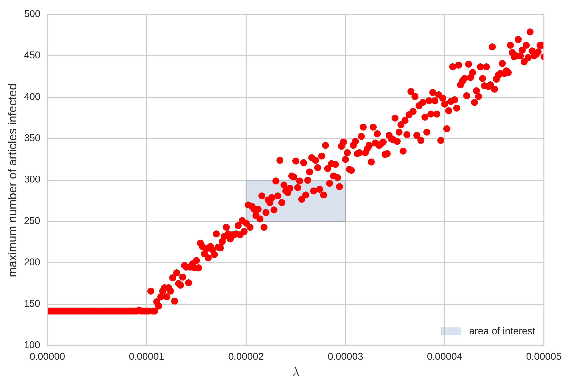
Looking at the publication date distribution (figure 9) we notice that the maximum number of articles published in a day was between 250 and 300. We derive the simulation parameters from this distribution. For example, on figure 10 we plot the peak of the infection for a range() of values. From that distribution of peak magnitudes we selected a lambda to match the empirical peak: .

432
From the simulation (figure 11) we obtain the state matrix, which we use to compare the simulated infection distribution with the original data. Then we ran 10 thousand simulations to show that the model proposed matches the real world dynamics of news articles influences (figure 12).


4 Discussion
In this paper, we presented a methodology for reconstructing the network representing the spread of news in digital media. The results proposed started from a well defined subset of articles with high semantic similarities. However we believe the criteria of similarity used to reconstruct the network would work even on a random sample or articles, provided that it was large enough to contain a good portion of the putative spread network one is trying to characterize. In other words, the reconstruction algorithm can be used to detect contagious structures within any large enough collection of news articles.
We also demonstrated that a classical SIR process over the network is driving the spread dynamics. This means that the if one is able to observe the start of the spread, the overall reach and time of persistence in the media can be predicted from analytical results available for the SIR model.
The news subject selected, "Charlie Hebdo attack", represents a very spontaneous media coverage given the great surprise with which it happened, but also due the homogeneous response of the global media condemning the cowardly attack. We believe that deviations from the classical SIR dynamics shown here can hint at some form of media manipulation, but that hypothesis remains to be tested based on well defined cases, such as purchased media coverage during political campaigns, etc. With the current concerns about “fake" media pieces 8, Perhaps the methods presented here can help to discriminate authentic media articles from fake ones based on their spread dynamics or influence patterns. We already began to see some attempts to automatically detect fake news 9, 10, but they mostly rely on linguistic cues. We believe that qualitative and quantitative aspects of the spread networks can also be of use.
References
- [1] A. Hermida, F. Fletcher, D. Korell, D. Logan, Share, like, recommend: Decoding the social media news consumer, Journalism Studies 13 (2012) 815–824.
- [2] D. M. Romero, W. Galuba, S. Asur, B. A. Huberman, Influence and passivity in social media, in: Machine learning and knowledge discovery in databases, Springer, 2011, pp. 18–33.
- [3] R. Pastor-Satorras, C. Castellano, P. Van Mieghem, A. Vespignani, Epidemic processes in complex networks, Reviews of modern physics 87 (2015) 925.
- [4] L. M. Bettencourt, A. Cintrón-Arias, D. I. Kaiser, C. Castillo-Chávez, The power of a good idea: Quantitative modeling of the spread of ideas from epidemiological models, Physica A: Statistical Mechanics and its Applications 364 (2006) 513–536.
- [5] R. Mihalcea, C. Corley, C. Strapparava, Corpus-based and knowledge-based measures of text semantic similarity, in: AAAI, volume 6, pp. 775–780.
- [6] T. Mikolov, K. Chen, G. Corrado, J. Dean, Efficient estimation of word representations in vector space, arXiv preprint arXiv:1301.3781 (2013).
- [7] D. Hiemstra, A probabilistic justification for using tf idf term weighting in information retrieval, International Journal on Digital Libraries 3 (2000) 131–139.
- [8] D. Berkowitz, D. A. Schwartz, Miley, cnn and the onion: When fake news becomes realer than real, Journalism Practice 10 (2016) 1–17.
- [9] Z. Jin, J. Cao, Y. Zhang, J. Zhou, Q. Tian, Novel visual and statistical image features for microblogs news verification, IEEE Transactions on Multimedia (2016).
- [10] V. L. Rubin, N. J. Conroy, Y. Chen, S. Cornwell, Fake news or truth? using satirical cues to detect potentially misleading news. (????).