Alpha Fair Coded Caching

Since coded caching was first proposed [2] and its potential was recognized by the community, substantial efforts have been devoted to quantify the gain in realistic scenarios, including decentralized placement [6], non-uniform popularities [5, 7], and device-to-device (D2D) networks [4]. A number of recent works replace the original perfect shared link with wireless channels [9, 10, 11]. Commonly in the works with wireless channels, the performance of coded caching is limited by the user in the worst channel condition because the wireless multicast capacity is determined by the worst user [13, Chapter 7.2]. This limitation of coded caching has been recently highlighted in [11], while similar conclusions and some directions are given in [9, 10]. Our work is the first to addresses this aspect by jointly designing the transmissions over the broadcast channel and scheduling appropriate subsets of users.

Most past works deal with offline caching in the sense that both cache placement and delivery phases are performed once and do not capture the random and asynchronous nature of video traffic. The papers [8, 12] addressed partly the online nature by studying cache eviction strategies, and delay aspects. In this paper, we explore a different online aspect. Requests for video files arrive in an online fashion, and transmissions are scheduled over time-varying wireless channels.

Online transmission scheduling over wireless channels has been extensively studied in the context of opportunistic scheduling [17] and network utility maximization [14]. Prior works emphasize two fundamental aspects: (a) the balancing of user rates according to fairness and efficiency considerations, and (b) the opportunistic exploitation of the time-varying fading channels. Related to our work are the studies of wireless downlink with broadcast degraded channels; [21] gives a maxweight-type of policy and [22] provides a throughput optimal policy based on a fluid limit analysis. Our work is the first to our knowledge that studies coded caching in this setting. The new element in our study is the joint consideration of user scheduling with codeword construction for the coded caching delivery phase.

The performance metric is the time average delivery rate of files to user $k$, denoted by $\overline{r}_{k}$. Hence our objective is expressed with respect to the vector of delivery rates $\boldsymbol{r}$. We are interested in the fair file delivery problem:

where $\Lambda$ denotes the set of all feasible delivery rate vectors–clarified in the following subsection–and the utility function corresponds to the alpha fair family of concave functions obtained by choosing:

for some arbitrarily small $d>0$ (used to extend the domain of the functions to $x=0$). Tuning the value of $\alpha$ changes the shape of the utility function and consequently drives the system performance $\overline{\boldsymbol{r}}^{*}$ to different points: (i) $\alpha=0$ yields max sum delivery rate, (ii) $\alpha\to\infty$ yields max-min delivery rate [15], (iii) $\alpha=1$ yields proportionally fair delivery rate [16]. Choosing $\alpha\in(0,1)$ leads to a tradeoff between max sum and proportionally fair delivery rates.

The optimization (1) is designed to allow us tweak the performance of the system; we highlight its importance by an example. Suppose that for a 2-user system $\Lambda$ is given by the convex set shown on figure 1.

Different boundary points are obtained as solutions to (1). If we choose $\alpha=0$, the system is operated at the point that maximizes the sum $\overline{r}_{1}+\overline{r}_{2}$. The choice $\alpha\to\infty$ leads to the maximum $r$ such that $\overline{r}_{1}=\overline{r}_{2}=r$, while $\alpha=1$ maximizes the sum of logarithms. The operation point A is obtained when we always broadcast to all users at the weakest user rate and use [2] for coded caching transmissions. Note that this results in a significant loss of efficiency due to the variations of the fading channel, and consequently A lies in the interior of $\Lambda$. We may infer that the point $\alpha\to\infty$ is obtained by avoiding transmissions to users with instantaneous poor channel quality but still balancing their throughputs in the long run.

To analyze the set of feasible rate vectors $\Lambda$ we need to zoom in the detailed model of transmissions.

Caching model. There are $N$ equally popular files $W_{1},\dots,W_{N}$, each $F$ bits long. The files are available to the base station. User $k$ is equipped with cache memory $Z_{k}$ of $MF$ bits, where $M\in[0,N]$. Caching placement is performed during off-peak hour, and the goal is to fill the caches up to the memory constraint with selected bits. To this end, we need to select $K$ caching functions $\phi_{k}:\mbox{\bb F}_{2}^{NF}\to\mbox{\bb F}_{2}^{MF}$ which map the files $W_{1},\dots,W_{N}$ into the cache contents

The caching functions can be used to cache a few entire files, or a small fraction from each file, or even coded combinations of subfiles [2, 8]. It is important to note that the caching functions are selected once, without knowledge of future requests, and are fixed throughout our system operation.¹¹ 1 A reasonable extension is to enable infrequent updates of the caching placement phase.

Downlink channel model. We consider a standard block-fading broadcast channel, such that the channel state remains constant over a slot of $T_{\rm slot}$ channel uses and changes from one slot to another in an i.i.d. manner. The channel output of user $k$ in any channel use of slot $t$ is given by

where the channel input $\boldsymbol{x}\in\mbox{\bb C}^{T_{\rm slot}}$ is subject to the power constraint $\mbox{\bb E}[\|\boldsymbol{x}\|^{2}]\leq PT_{\rm slot}$; $\hbox{\boldmath$\nu$}_{k}(t)\sim{\cal N}_{\mbox{\bb C}}(0,{\bf I}_{T_{\rm slot}})$ are additive white Gaussian noises with covariance matrix identity of size $T_{\rm slot}$, assumed independent of each other; $\{h_{k}(t)\in\mbox{\bb C}\}$ are channel fading coefficients $\sim\beta_{k}^{2}\text{exp}(1)$ independently distributed across time and users, with $\beta_{k}$ denoting the path-loss parameter of user $k$.

Encoding and transmissions. The transmissions aim to contribute information towards the delivery of a specific vector of file requests $\boldsymbol{d}(t)$, where $d_{k}(t)\in\{1,\dots,N\}$ denotes the index of the requested file by user $k$ in slot $t$. Here $N$ is the video library size, typically in the order of 10K. The requests are generated randomly, and whenever a file is delivered to user $k$, the next request of this user will be for another randomly selected file.

At each time slot, the base station observes the channel state $\boldsymbol{h}(t)=(h_{1}(t),\dots,h_{K}(t))$ and the request vector up to $t$, $\boldsymbol{d}^{t}$, constructs a transmit symbol using the encoding function $f_{t}:\{1,..,N\}^{Kt}\times\mbox{\bb C}^{K}\to\mbox{\bb C}^{T_{\rm slot}}$.

Finally, it transmits a codeword $\boldsymbol{x}(t)$ for the $T_{\rm slot}$ channel uses over the fading broadcast channel in slot $t$ . The encoding function may be chosen at each slot to contribute information to a selected subset of users $\mathcal{J}(t)\subseteq\{1,\dots,K\}$. This allows several possibilities, e.g. to send more information to a small set of users with good instantaneous channel qualities, or less information to a large set that includes users with poor quality.

Decoding. At slot $t$, each user $k$ observes the local cache contents $Z_{k}$ and the sequence of channel outputs so far $y_{k}(\tau),~~\tau=1,\dots,t$ and employs a decoding function $\xi_{k}$ to determine the decoded files. Let $D_{k}(t)$ denote the number of files decoded by user $k$ after $t$ slots. The decoding function $\xi_{k}$ is a mapping

The decoded files of user $k$ at slot $t$ are given by $\xi_{k}(y_{k}^{T_{\rm slot}t},Z_{k},\boldsymbol{h}^{t},\boldsymbol{d}^{t})$, and depend on the channel outputs and states up to $t$, the local cache contents, and the requested files of all users up to $t$. A file is incorrectly decoded if it does not belongs to the set of requested files. The number of incorrectly decoded files are then given by $|\cup_{t}\{\xi_{k}(t)\}\setminus d_{k}^{t}|$ and the number of correctly decoded files at time $t$ is:

In contrast to past works which study the performance of one-shot coded caching [2, 6, 8], our rate metric measures the ability of the system to continuously deliver files to users.

Finding the optimal policy is very complex. In this paper, we restrict the problem to specific class of policies given by the following mild assumptions:

Since we restrict our action space, the delivery rate feasibility region, $\Lambda^{CC}$, of the class of policies $\Pi^{CC}$ is smaller than the one for the original problem $\Lambda$. However, these restrictions allow us to come up with a concrete solution approach. Note that the optimal cache and transmission design policy is already a very hard problem even in the simple case of broadcast transmissions with a fixed common rate, and the method in [2], [6] are practical approaches with good performance. In addition, looking at demand IDs when combining files would be very complex and, because of the big library sizes, is not expected to bring substantial gains (it is improbable that two users will make request for the same file in close time instances).

At each time slot $t$, the controller admits $a_{k}(t)$ files to be delivered to user $k$, and hence $a_{k}(t)$ is a control variable.²² 2 We note that random file arrivals can be directly captured with the addition of an extra queue [14], which we avoid to simplify exposition. As our model dictates, the succession of requested files for user $k$ is determined uniformly at random.

Queueing model. The base station organizes the information into the following types of queues:

1. 1.

   User queues to store admitted files, one for each user. The buffer size of queue $k$ is denoted by $S_{k}(t)$ and expressed in number of files.

2. 2.

   Codeword queues to store codewords to be multicast. There is one codeword queue for each subset of users ${\cal J}\subseteq\{1,\dots,K\}$. The size of codeword queue ${\cal J}$ is denoted by $Q_{{\cal J}}(t)$ and expressed in bits.

A queueing policy $\pi$ performs the following operations: (i) decides how many files to admit into the user queues $S_{k}(t)$ in the form of $(a_{k}(t))$ variables, (ii) then it decides how to combine together files from different user queues to be encoded into the form of multiple codewords which represent the required broadcast transmissions for the reception of this file–these codewords are stored in the appropriate codeword queues $Q_{{\cal J}}(t)$, (iii) and last it decides the encoding function $f_{t}$. (ii) and (iii) are further clarified in the next section.

The above definition implies that the average delay of each job in the queue is finite.

In our problem, if we develop a policy that keeps user queues $\boldsymbol{S}(t)$ stable, then all admitted files will, at some point, be combined into codewords. If in addition codeword queues $\boldsymbol{Q}(t)$ are stable, then all generated codewords will reach their destinations, meaning that all receivers will be able to decode the admitted files that they requested.

Let $\overline{a}_{k}=\limsup\limits_{t\rightarrow\infty}\frac{1}{t}\sum_{t=0}^{t-1}\mathbb{E}\left[a_{k}(t)\right],$ denote the time average number of admitted files for user $k$. Lemma 3 implies the following Corollary.

Contrary to the offline coded caching in [6], we propose an online delivery scheme consisting of the following three blocks. Each block is operated at each slot.

1. 1.

   Admission control: At the beginning of each slot, the controller decides how many requests for each user, $a_{k}(t)$ should be pulled into the system from the infinite reservoir.

2. 2.

   Routing: The cumulative accepted files for user $k$ are stored in the admitted demand queue whose size is given by $S_{k}(t)$ for $k=1,\dots,K$. The server decides the combinations of files to perform coded caching. The decision at slot $t$ for a subset of users ${\cal J}\subseteq\{1,..,K\}$, denoted by $\sigma_{{\cal J}}(t)\in\{0,1,\dots,\sigma_{\max}\}$, refers to the number of combined requests for this subset of users. It is worth noticing that offline coded caching lets $\sigma_{{\cal J}}=1$ for ${\cal J}=\{1,\dots,K\}$ and zero for all the other subsets. The size of the queue $S_{k}$ evolves as:

   $\displaystyle S_{k}(t+1)=\left[S_{k}(t)-\sum_{{\cal J}:k\in{\cal J}}\sigma_{{\cal J}}(t)\right]^{+}+a_{k}(t)$

   (16)

   If $\sigma_{{\cal J}}(t)>0$, the server creates codewords by applying offline coded caching explained in Section [] for this subset of users as a function of the cache contents $\{Z_{j}:j\in{\cal J}\}$.

3. 3.

   Scheduling: The codewords intended to the subset ${\cal J}$ of users are stored in codeword queue whose size is given by $Q_{{\cal I}}(t)$ for ${\cal I}\subseteq\{1,\dots,K\}$. Given the instantaneous channel realization $\boldsymbol{h}(t)$ and the queue state $\{Q_{{\cal I}}(t)\}$, the server performs scheduling and rate allocation. Namely, at slot $t$, it determines the number $\mu_{{\cal I}}(t)$ of bits per channel use to be transmitted for the users in subset ${\cal I}$. By letting $b_{{\cal J},{\cal I}}$ denote the number of bits generated for codeword queue ${\cal I}\subseteq{\cal J}$ when offline coded caching is performed to the users in ${\cal J}$, codeword queue ${\cal I}$ evolves as

   $\displaystyle Q_{{\cal I}}(t+1)=\left[Q_{{\cal I}}(t)-T_{\rm slot}\mu_{{\cal I}}(t)\right]^{+}+\sum_{{\cal J}:{\cal I}\subseteq{\cal J}}b_{{\cal J},{\cal I}}\sigma_{{\cal J}}(t)$

   where $b_{{\cal J},{\cal I}}=m^{|{\cal I}|}(1-m)^{|{\cal J}|-|{\cal I}|-1}$.

In order determine our proposed policy, namely the set of decisions $\{\boldsymbol{a}(t),\hbox{\boldmath$\sigma$}(t),\hbox{\boldmath$\mu$}(t)\}$ at each slot $t$, we first characterize the feasible region $\Lambda$ as a set of arrival rates $\boldsymbol{a}$. We let $\pi_{\mathbf{h}}$ denote the probability that the channel state at slot $t$ is $\boldsymbol{h}\in{\cal H}$ where ${\cal H}$ is the set of all possible channel states. We let $\Gamma(\boldsymbol{h})$ denote the capacity region for a fixed channel state $\mathbf{h}$. Then we have the following

Constraint (17) says that the service rate at which admitted demands are combined to form codewords is greater than the arrival rate, while (18) implies that the long-term average transmission rate $\overline{\mu}_{{\cal I}}$ for the subset ${\cal I}$ of users should be higher than the rate at which bits of generated codewords for this group arrive. In terms of the queueing system defined, these constraints impose that the service rates of each queue should be greater than their arrival rates, thus rendering them stable.

Theorem 5 implies that the set of feasible average delivery rates is a convex set.

In order to perform the utility maximization (15), we need to introduce one more set of queues. These queues are virtual, in the sense that they do not hold actual file demands or bits, but are merely counters to drive the control policy. Each user $k$ is associated with a queue $U_{k}(t)$ which evolves as follows:

where $\gamma_{k}(t)$ represents the arrival process to the virtual queue and is given by

In the above, $V>0$ is a parameter that controls the utility-delay tradeoff achieved by the algorithm (see Theorem 6).

The general intuition here is as follows: Observe that the number $a_{k}(t)$ of admitted demands is the service rate for the virtual queues $U_{k}(t)$. The control algorithm actually seeks to optimize the time average of the virtual arrivals $\gamma_{k}(t)$. However, since $U_{k}(t)$ is stable, its service rate, which is the actual admission rate, will be greater than the rate of the virtual arrivals, therefore giving the same optimizer. Stability of all other queues will guarantee that admitted files will be actually delivered to the users.

We present our on-off policy for admission control and routing. For every user $k$, admission control chooses $a_{k}(t)$ demands given by

For every subset ${\cal J}\subseteq\{1,\dots,K\}$, routing combines $\sigma_{{\cal J}}(t)$ demands of users in ${\cal J}$ given by

In order to stabilize all codeword queues, the scheduling and resource allocation explicitly solve the following weighted sum rate maximization at each slot $t$ where the weight of the subset ${\cal J}$ corresponds to the queue length of $Q_{{\cal J}}$

We propose to apply the power allocation algorithm in Section IV to solve the above problem by sorting users in a decreasing order of channel gains and treating $Q_{{\cal J}}(t)$ as $\theta_{{\cal J}}$. In adition, we assume that the number of channel uses in one coherence block is large enough such that the decoding error from choosing channel codes with rate $\hbox{\boldmath$\mu$}(t)$ is very small. In this case, no feedback from the receivers is given.

We conclude this section by providing an example of our proposed online delivery network for $K=3$ users as illustrated in Fig. 3.

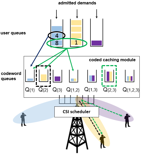
At slot $t$ the server decides to combine $W_{1}$ requested by user $2$ with $W_{8}$ requested by user $2$ and to process $W_{4}$ requested by user $1$ uncoded. Therefore $\sigma_{\{1,2\}}(t)=\sigma_{\{1\}}(t)=1$ and $\sigma_{{\cal J}}(t)=0$ otherwise. Given this codeword construction, codeword queues have inputs as described in Table I.

In addition, data from queues $Q_{\{2\}}(t),Q_{\{2.3\}}(t)$ are transmitted.

References

- [1] “White paper: Cisco VNI Forecast and Methodology, 2015-2020”, Tech. Report, 2015.
- [2] M. Maddah-Ali and U. Niesen, “Fundamental Limits of Caching,” IEEE Trans. Inf. Theory, vol. 60, no. 5, pp. 2856–2867, 2014.
- [3] G. S. Paschos, E. Bastug, I. Land, G. Caire, and M. Debbah, “Wireless caching: technical misconceptions and business barriers”, IEEE Communications Magazine, 2016.
- [4] M. Ji, G. Caire, A. Molisch, “Fundamental Limits of Distributed Caching in D2D Wireless Networks” , arXiv/1304.5856, 2013.
- [5] M. Ji, A. Tulino, J. Llorca, and G. Caire, “Order-Optimal Rate of Caching and Coded Multicasting with Random Demands”, arXiv:1502.03124, 2015.
- [6] M. Maddah-Ali and U. Niesen, “Decentralized Coded Caching Attains Order-Optimal Memory-Rate Tradeoff”, IEEE/ACM Trans. Netw., vol. 23, no. 4, pp. 1029–1040, 2015.
- [7] M. Maddah-Ali and U. Niesen, “Coded Caching with Nonuniform Demands”, in IEEE INFOCOM Workshops, 2014.
- [8] R. Pedarsani, M. Maddah-Ali, and U. Niesen, “Online Coded Caching,” in IEEE/ACM Trans. Netw., vol. 24, no. 2, pp. 836-845, 2016.
- [9] J. Zhang, and P. Elia, ”Wireless Coded Caching: a Topological Perspective”. arXiv:1606.08253, 2016.
- [10] S. S. Bidokhti, M. Wigger, and R. Timo, “Noisy Broadcast Networks with Receiver Caching”, arXiv preprint arXiv:1605.02317, 2016.
- [11] K-H. Ngo, S. Yang, and M. Kobayashi, “Cache-Aided Content Delivery in MIMO Channels”, in Proc. Allerton, IL, USA, 2016.
- [12] U. Niesen M. Maddah-Ali “Coded Caching for Delay-Sensitive Content”, in IEEE ICC, pp. 5559-5564, 2015.
- [13] A. El Gamal and Y. H. Kim, “Network Information Theory”, Cambridge university press, 2011.
- [14] M. Neely, “Stochastic Network Optimization with Application to Communication and Queueing Systems”, Morgan & Claypool, 2010.
- [15] J. Mo and J. Walrand, “Fair end-to-end window-based congestion control”, IEEE/ACM Trans. Netw. , Vol. 8, No. 5, Oct. 2000.
- [16] F. Kelly, “Charging and Rate Control for Elastic Traffic”, European Transactions on Telecommunications, 1997.
- [17] A. L. Stolyar, “On the asymptotic optimality of the gradient scheduling algorithm for multiuser throughput allocation.” Operations Research Vol. 53 No. 1, 2005.
- [18] R. Knopp and P. A. Humblet, “Information capacity and power control in single-cell multiuser communications,” in IEEE ICC, Seattle, WA, 1995.
- [19] H. Shirani-Mehr, G. Caire and M. J. Neely, “MIMO Downlink Scheduling with Non-Perfect Channel State Knowledge,” in IEEE Trans. Commun. , vol. 58, no. 7, pp. 2055-2066, July 2010.
- [20] G. Caire, R. R. Muller and R. Knopp, “Hard Fairness Versus Proportional Fairness in Wireless Communications: The Single-Cell Case,” in IEEE Trans. Inf. Theory, vol. 53, no. 4, pp. 1366-1385, April 2007.
- [21] K. Seong, R. Narasimhan, and J. Cioffi, “Queue Proportional Scheduling via Geometric Programming in Fading Broadcast Channels”, in IEEE JSAC, vol. 24, no. 8, Aug 2006.
- [22] A. Eryilmaz, and R. Srikant, and J. R. Perkins, “Throughput-optimal Scheduling for Broadcast Channels”, in Proc. ITCom, Denver, CO, August 2001.
- [23] D. Tse, “Optimal Power Allocation over Parallel Gaussian Broadcast Channels”, unpublished
- [24] M. Neely, E. Modiano, and C.-P. Li, “Fairness and Optimal Stochastic Control for Heterogeneous Networks”, IEEE/ACM Trans. Netw., 2005.