跳到论文正文
W Papers独立论文阅读器 arXiv:1701.07617 论文正文 计算阅读时间 · 0%
引用这篇论文根据当前论文元数据生成,正式投稿前建议核对。


License: arXiv.org perpetual non-exclusive license
arXiv:1701.07617v1 [math.DS] 26 Jan 2017

Limiting curves for polynomial adic systems.

Supported by the RFBR (grant 14-01-00373)
A. R. Minabutdinov ††thanks: National Research University Higher School of Economics, Department of Applied Mathematics and Business Informatics, St.Petersburg, Russia, e-mail: aminabutdinov@hse.ru.
Abstract

We prove the existence and describe limiting curves resulting from deviations in partial sums in the ergodic theorem for cylindrical functions and polynomial adic systems. For a general ergodic measure-preserving transformation and a summable function we give a necessary condition for a limiting curve to exist. Our work generalizes results by É. Janvresse, T. de la Rue and Y. Velenik and answers several questions from their work.

Key words: Polynomial adic systems, ergodic theorem, deviations in ergodic theorem.

MSC: 37A30, 28A80

1 Introduction

In this paper we develop the notion of a limiting curve introduced by É. Janvresse, T. de la Rue and Y. Velenik in [16]. Limiting curves were studied for the Pascal adic in [16] and [11]. In this paper we study it for a wider class of adic transformations.

Let TT be a measure preserving transformation defined on a Lebesgue probability space (X,ℬ,μ)(X,\mathcal{B},\mu) with an invariant ergodic probability measure μ\mu. Let gg denote a function in L1​(X,μ)L^{1}(X,\mu). Following [16] for a point x∈Xx\in X and a positive integer jj we denote the partial sum ∑k=0j−1g⁡(Tk​x)\sum\limits_{k=0}^{j-1}g\big(T^{k}x\big) by Sxg​(j)S_{x}^{g}(j). We extend the function Sxg​(j)S_{x}^{g}(j) to a real valued argument by a linear interpolation and denote extended function by Fxg​(j)F_{x}^{g}(j) or simply F⁡(j),j≥0F(j),j\geq 0.

Let (ln)n=1∞(l_{n})_{n=1}^{\infty} be a sequence of positive integers. We consider continuous on [0,1][0,1] functions φn​(t)=F⁡(t⋅ln​(x))−t⋅F⁡(ln)Rn(≡φx,lng​(t)),\varphi_{n}(t)=\frac{F(t\cdot l_{n}(x))-t\cdot F(l_{n})}{R_{n}}\big(\equiv\varphi_{x,l_{n}}^{g}(t)\big), where the normalizing coefficient RnR_{n} is canonically defined to be equal to the maximum in t∈[0,1]t\in[0,1] of |F⁡(t⋅ln​(x))−t⋅F⁡(ln)||F(t\cdot l_{n}(x))-t\cdot F(l_{n})|.

Definition 1.

If there is a sequence lng​(x)∈ℕl^{g}_{n}(x)\in\mathbb{N} such that functions φx,lng​(x)g\varphi_{x,l^{g}_{n}(x)}^{g} converge to a (continuous) function φxg\varphi_{x}^{g} in sup-metric on [0,1],[0,1], then the graph of the limiting function φ=φxg\varphi=\varphi^{g}_{x} is called a limiting curve, sequence ln=lng​(x)l_{n}=l_{n}^{g}(x) is called a stabilizing sequence and the sequence Rn=Rx,lng​(x)gR_{n}=R_{x,l^{g}_{n}(x)}^{g} is called a normalizing sequence. The quadruple (x,(ln)n=1∞,(Rn)n=1∞,φ)\Big(x,\big(l_{n}\big)_{n=1}^{\infty},\big(R_{n}\big)_{n=1}^{\infty},\varphi\Big) is called a limiting bridge.

Heuristically, the limiting curve describes small fluctuations (of certainly renormalized) ergodic sums 1l​F​(l),l∈(ln),\frac{1}{l}F(l),l\in(l_{n}), along the forward trajectory x,T⁡(x),T2​(x)​…x,T(x),T^{2}(x)\dots. More specifically, for l∈(ln)l\in(l_{n}) it holds F⁡(t⋅l)=t​F​(l)+Rl​φ​(t)+o⁡(Rl)F(t\cdot l)=tF(l)+R_{l}\varphi(t)+o(R_{l}), where t∈[0,1].t\in[0,1].

In this paper we will always assume that TT is an adic transformation. Adic transformations were introduced into ergodic theory by A. M. Vershik in  [1] and were extensively studied since that time. The following important theorem shows that adicity assumption is not restrictive at all:

Theorem.

(A. M. Vershik, [2]). Any ergodic measure preserving transformation on a Lebesgue space is isomorphic to some adic transformation. Moreover, one can find such an isomorphism that any given countable dense invariant subalgebra of measurable sets goes over into the algebra of cylinder sets.

In [2, 3, 5] authors encouraged studying different approaches to combinatorics of Markov’s compacts (sets of paths in Bratteli diagrams). In particular, it is interesting to find a natural class of adic transformations such that the limiting bridges exist for cylindric functions. Moreover, it is interesting to study joint growth rates of stabilizing and normalizing sequences.

In this paper we give necessary condition for a limiting curve to exist. Next we find necessary and sufficient conditions for almost sure (in xx) existence of limiting curves for a class of self-similar adic transformations and cylindric functions. These transformations (in a slightly less generality) were considered by X. Mela and S. Bailey in [19] and [12]. Our work extends [16] and answers several questions from this research.

2 Limiting curves and cohomologous to a constant functions

In this section we show that a necessary condition for limiting curves to exist is unbounded growth of the normalizing coefficient RnR_{n}. Contrariwise we show that normalizing coefficients are bounded if and only if function gg is cohomologous to a constant. In particular this implies that there are no limiting curves for cylindric functions for an ordinary odometer.

2.1 Notions and definitions

Let B=B⁡(𝒱,ℰ)B=B(\mathcal{V},\mathcal{E}) denote a Bratteli diagram defined by the set of vertices 𝒱\mathcal{V} and the set of edges ℰ\mathcal{E}. Vertices at the level nn are numbered k=0k=0 through L⁡(n)L(n). We associate to a Bratteli diagram BB the space X=X⁡(B)X=X(B) of infinite edge paths beginning at the vertex v0=(0,0).v_{0}=(0,0). Following fundamental paper [1] we assume that there is a linear order ≤n,k\leq_{n,k} defined on the set of edges with a terminate vertex (n,k),0≤k≤L⁡(n)(n,k),0\leq k\leq L(n). These linear orders define a lexicographical order on the set of edges paths in XX that belong to the same class of the tail partition. We denote by ⪯\preceq corresponding partial order on XX. The set of maximal (minimal) paths is defined by XmaxX_{\max} (correspondingly, XminX_{\min}).

Definition 2.

Adic transformation TT is defined on X∖(Xmax∪Xmin)X\setminus\big(X_{\max}\cup X_{\min}\big) by setting T​x,x∈X,Tx,\,x\in X, equal to the successor of xx, that is, the smallest yy that satisfies y≻xy\succ x.

Let ω\omega be a path in XX. We denote by (n,kn​(ω))(n,k_{n}(\omega)) a vertex through which ω\omega passes at level nn. For a finite path c=(c1,…,cn)c=(c_{1},\dots,c_{n}) we denote kn​(c)k_{n}(c) simply by k⁡(c)k(c). A cylinder set C=[c1c2…cn]={ω∈X|ω1=c1,ω2=c2,…,ωn=cn}C=[c_{1}c_{2}\dots c_{n}]=\{\omega\in X|\omega_{1}=c_{1},\omega_{2}=c_{2},\dots,\omega_{n}=c_{n}\} of a rank nn is totally defined by a finite path from the vertex (0,0)(0,0) to the vertex (n,k)=(n,k⁡(c)).(n,k)=(n,k(c)). Sets πn,k\pi_{n,k} of lexicographically ordered finite paths c=(c0,c1,…,cn−1)c=(c_{0},c_{1},\dots,c_{n-1}), k⁡(c)=nk(c)=n, are in one to one correspondence with towers τn,k\tau_{n,k} made up of corresponding cylinder sets Cj=τn,k​(j),1⩽j⩽dim(n,k)C_{j}=\tau_{n,k}(j),1\leqslant j\leqslant\dim(n,k). The dimension dim(n,k)\dim(n,k) of the vertex (n,k)(n,k) is the total number of such finite paths (rungs of the tower).

We denote by Num​(c)\text{Num}(c) the number of finite paths in lexicographically ordered set πn,k\pi_{n,k}. Evidently, 1≤Num​(c)≤dim(n,k).1\leq\text{Num}(c)\leq\dim(n,k). For a given level nn the set of towers {τn,k}0≤k≤L⁡(n)\{\tau_{n,k}\}_{0\leq k\leq L(n)} defines approximation of transformation TT, see [1], [3].

We can consider a vertex (n,k)(n,k) of Bratteli diagram BB as an origin in a new diagram Bn,k′=(𝒱′,ℰ′)B^{\prime}_{n,k}=(\mathcal{V}^{\prime},\mathcal{E}^{\prime}). The set of vertices 𝒱′\mathcal{V}^{\prime}, edges ℰ′\mathcal{E}^{\prime} and edges paths X⁡(Bn,k′)X(B^{\prime}_{n,k}) are naturally defined. As above partial order ⪯′\preceq^{\prime} on X⁡(B′)X(B^{\prime}) is induced by linear orders ≤n′,k′,n′>n\leq_{n^{\prime},k^{\prime}},n^{\prime}>n.

Definition 3.

Ordered Bratteli diagram (B,⪯)(B,\preceq) is self-similar if ordered diagrams (B,⪯)(B,\preceq) and (Bn,k′,⪯n,k′)(B^{\prime}_{n,k},\preceq^{\prime}_{n,k}) are isomorphic n∈ℕ,n\in\mathbb{N}, 0⩽k⩽L⁡(n).0\leqslant k\leqslant L(n).

Let ℱ\mathscr{F} denote the set of all functions f:X→ℝ.f:X\rightarrow\mathbb{R}. We denote by ℱN\mathscr{F}_{N} the space of cylindric functions of rank NN (i.e. functions that are constant on cylinders of rank NN).

Let g∈ℱN,N<n.g\in\mathscr{F}_{N},\ N<n. We denote by Fn,kgF_{n,k}^{g} linearly interpolated partial sums Sx∈τnk​(1)gS^{g}_{x\in\tau_{n}^{k}(1)}. Assume that self-similar Bratteli diagram BB has L+1L+1 vertices at level NN and let ω∈πn,k,0⩽k⩽L⁡(n),\omega\in\pi_{n,k},0\leqslant k\leqslant L(n), be a finite path such that its initial segment ω′=(ω1,ω2,…,ωN)\omega^{\prime}=(\omega_{1},\omega_{2},\dots,\omega_{N}) is a maximal path, i.e. Num​(ω′)=dim(N,k⁡(ω′))\text{Num}(\omega^{\prime})=\dim(N,k(\omega^{\prime})). Let En,kN,l{E}^{N,l}_{n,k} denote the number of paths from (0,0)(0,0) to (n,k)(n,k) passing through the vertex (N,l),0≤l≤L,(N,l),0\leq l\leq L, and not exceeding path ω\omega. We denote by ∂n,kN,l(ω){\partial}^{N,l}_{n,k}(\omega) the ratio of En,kN,l{E}^{N,l}_{n,k} to dim(N,l).\dim(N,l). It is not hard to see that a partial sum Fn,kgF_{n,k}^{g} evaluated at j=Num​(ω)j=\text{Num}(\omega) has the following expression:

Fn,kg​(j)=∑l=0LhN,lg​∂n,kN,l(ω),F^{g}_{n,k}(j)=\sum\limits_{l=0}^{L}h^{g}_{N,l}{\partial}^{N,l}_{n,k}(\omega), (1)

where coefficients hN,lgh^{g}_{N,l} are equal to FN,lg​(HN,l), 0⩽l⩽LF_{N,l}^{g}(H_{N,l}),\,0\leqslant l\leqslant L.

Expression (1) is a generalization of Vandermonde’s convolution formula.

2.2 A necessary condition for existence of limiting curves

Let (X,T)(X,T) be an ergodic measure-preserving transformation with invariant measure μ\mu. Let gg be a summable function and a point x∈Xx\in X. We consider a sequence of functions φx,lng\varphi^{g}_{x,l_{n}} and normalizing coefficients Rx,lngR_{x,l_{n}}^{g} given by the identity

φx,ln​(x)g​(t)=Sxg​([t⋅ln​(x)])−t⋅Sxg​(ln​(x))Rx,ln​(x)g,\varphi_{x,l_{n}(x)}^{g}(t)=\frac{S_{x}^{g}([t\cdot l_{n}(x)])-t\cdot S_{x}^{g}(l_{n}(x))}{R_{x,l_{n}(x)}^{g}},

where Rx,ln​(x)gR_{x,l_{n}(x)}^{g} equals maximum of absolute value of the numerator. Without loss of generality, we assume that the limit g∗​(x)=limn→∞1n​Sxgg^{*}(x)=\lim\limits_{n\rightarrow\infty}\frac{1}{n}S^{g}_{x} exists at the point xx. The following theorem generalizes Lemma 2.12.1 from [16] for an arbitrary summable function.

Theorem 1.

If a continuous limiting curve φxg=limnφx,lng\varphi_{x}^{g}=\lim_{n}\varphi^{g}_{x,l_{n}} exists for μ\mu-a.e. xx, then the normalizing coefficients Rx,lngR_{x,l_{n}}^{g} are unbounded in nn.

Proof.

Assume the contrary that |Rx,lng|⩽K|R_{x,l_{n}}^{g}|\leqslant K. For simplicity we introduce the following notation: S=Sxg,S=S_{x}^{g}, φn=φx,lng,\varphi_{n}=\varphi^{g}_{x,l_{n}}, Rn=Rx,lngR_{n}=R_{x,l_{n}}^{g} and φ=φx\varphi=\varphi_{x}. Since φ≠0,\varphi\neq 0, there is j∈ℕj\in\mathbb{N} such that 1j​S​(j)≠g∗.\frac{1}{j}S(j)\neq g^{*}. This in turn implies lim infn|φn​(jln)|=lim infn1Rn​|S⁡(j)−j​S​(ln)ln|⩾1K​|S⁡(j)−j​g∗|=jK|1j​S​(i)−g∗|>0,\liminf_{n}\big|\varphi_{n}(\frac{j}{l_{n}})\big|=\liminf_{n}\frac{1}{R_{n}}\big|S(j)-\frac{jS(l_{n})}{l_{n}}\big|\geqslant\frac{1}{K}|S(j)-jg^{*}|=\frac{j}{K}\big|\frac{1}{j}S(i)-g^{*}\big|>0, contradicting continuity of the limiting curve φ\varphi at the origin.

∎

Definition 4.

A function g∈L∞​(X,μ)g\in L^{\infty}(X,\mu) (μ\mu-a.e.) of the form g=c+h∘T−hg~=~c+h\circ T-h for some c∈ℝc\in\mathbb{R} and h∈L∞​(X,μ)h\in L^{\infty}(X,\mu) is called cohomologous to a constant in L∞L^{\infty}.

Theorem 2.

Normalizing sequence Rx,lngR_{x,l_{n}}^{g} is bounded if and only if function gg is cohomologous to a constant.

Proof.

Sums ∑j=0n−1(g−g∗)∘Tj\sum\limits_{j=0}^{n-1}(g-g^{*})\circ T^{j} of a cohomologous function are μ\mu-a.e. bounded, therefore normalizing coefficients Rx,lngR_{x,l_{n}}^{g} are μ\mu-a.e. bounded too.

The proof of the converse statement exploits the result by A. G. Kachurovskiy from [7]. Assume that the normalizing coefficients Rx,lngR_{x,l_{n}}^{g} are bounded. Then for μ\mu-a.e. point x∈Xx\in X and for any j∈ℕj\in\mathbb{N} the following inequality holds |Sxg​(j)−jln​Sxg​(ln)|⩽C|S^{g}_{x}(j)-\frac{j}{l_{n}}S^{g}_{x}(l_{n})|\leqslant C. Going to the limit in nn, we see that |∑i=1jf∘Ti​(x)|⩽C,|\sum\limits_{i=1}^{j}f\circ T^{i}(x)|\leqslant C, where f=g−g∗f=g-g^{*}. Theorem 1919 from [7] (see also G. Halasz, [14]), inequality |Sxf|⩽C,|S^{f}_{x}|\leqslant C, is equivalent to existence of a function h∈L∞h\in L^{\infty}, such that f=h∘T−h.f=h\circ T-h. Therefore gg equals to h∘T−h+g∗.h\circ T-h+g^{*}. ∎

Definition 5.

Let BB be a Bratteli diagram such that there is only one vertex at each level, and let the edge ordering be such that the edges increase from left to right. This transformation is called an odometer. A stationary odometer is an odometer for which the number of edges connecting consecutive levels is constant.

Figure 1: A Bratteli diagram of an odometer.
Theorem 3.

Let (X,T)(X,T) be an odometer. Any cylindric function g∈ℱNg\in\mathscr{F}_{N} is cohomologous to a constant. Therefore there is no limiting curve for a cylindric function.

Proof.

There is only one vertex (n,0)(n,0) at each level n.n. Expression  (1) for the partial sum Fn,0g​(i)F_{n,0}^{g}(i) is evidently valid for any odometer (even without assumption of self-similarity). Moreover, expression (1) is defined by the only coefficient hN,0gh^{g}_{N,0} and therefore is proportional to HN=dim(N,0)H_{N}=\dim(N,0). We can subtract such constant CC to the function gg that equality hN,0g−C=0h^{g-C}_{N,0}=0 holds. But this is equivalent to the following: The function function g−Cg-C belongs to the linear space spanned by the functions fj−fj∘T,1⩽j⩽HN,f_{j}-f_{j}\circ T,1\leqslant j\leqslant H_{N}, where fjf_{j} is the indicator-function of the jj-th rung in the tower τN,0\tau_{N,0}. Therefore function g−Cg-C is cohomologous to zero. ∎

3 Existence of limiting curves for polynomial adic systems

In this part we will show that any not cohomologous to a constant cylindric function in a polynomial adic system has a limiting curve. These generalizes Theorem 2.4. from [16].

3.1 Polynomial adic systems

Let p⁡(x)=a0+a1​x​⋯+ad​xdp(x)=a_{0}+a_{1}x\dots+a_{d}x^{d} be an integer polynomial of degree d∈ℕd\in\mathbb{N} with positive integer coefficients ai,0≤i≤d.a_{i},0\leq i\leq d. Bratteli diagram Bp=(𝒱,ℰ)pB_{p}=(\mathcal{V},\mathcal{E})_{p} associated to polynomial p⁡(x)p(x) is defined as follows:

  1. 1.

    Number of vertices grows linearly: |𝒱0|=1|\mathcal{V}_{0}|=1 è |𝒱n|=|𝒱n−1|+d=n​d+1,n∈ℕ|\mathcal{V}_{n}|=|\mathcal{V}_{n-1}|+d=nd+1,n\in\mathbb{N}.

  2. 2.

    If 0⩽j⩽d0\leqslant j\leqslant d vertices (n,k)(n,k) and (n+1,k+j)(n+1,k+j) are connected by aja_{j} edges.

Polynomial p⁡(x)p(x) is called a generating polynomial of the diagram BpB_{p}, see paper [12] by S. Bailey.

Figure 2: Bratteli diagram associated to polynomial 1+x+3​x2.1+x+3x^{2}.

Since the number of edges into vertex (n,k)(n,k) is exactly p⁡(1)=a0+a1+⋯+adp(1)=a_{0}+a_{1}+\dots+a_{d} it is natural to use the alphabet 𝒜={0,1,…,a0+a1+⋯+ad−1}\mathcal{A}=\{0,1,\dots,a_{0}+a_{1}+\dots+a_{d}-1\} for edges labeling. We call a lexicographical order defined in [12] a canonical order. It is defined as follows: Edges connecting (0,0)(0,0) with (1,d)(1,d) are labeled through 00 to ad−1a_{d}-1 (from left to right); edges connecting (0,0)(0,0) and (1,d−1)(1,d-1), are indexed by ada_{d} to ad+ad−1−1a_{d}+a_{d-1}-1, etc. Edges connecting (0,0)(0,0) and (1,0)(1,0), are indexed through a0+a1+⋯+ad−1a_{0}+a_{1}+\dots+a_{d-1} to a0+a1+⋯+ada_{0}+a_{1}+\dots+a_{d}.

Infinite paths are totally defined by this labeling and may be considered as one sided infinite sequences in 𝒜ℕ.\mathcal{A}^{\mathbb{N}}. We denote the path space by Xp.X_{p}.

Figure 3: Labeling of the polynomial system associated to 1+x+3​x2.1+x+3x^{2}.

We denote by TpT_{p} the adic transformation associated with the canonical ordering.

Remark. Any self-similar Bratteli diagram is either a diagram of a stationary odometer or is associated to some polynomial p⁡(x)p(x). Any non-canonical ordering is obtained from canonical by some substitution σ\sigma.

Everywhere below we stick to the canonical order. Case of general order needs several straightforward changes that are left to the reader.

Dimension of the vertex (n,k)(n,k) from diagram BpB_{p} equals to the coefficient of xkx^{k} in the polynomial (p⁡(x))n(p(x))^{n} and is called generalized binomial coefficient. We denote it by Cp​(n,k)C_{p}(n,k). For n>1n>1 coefficients Cp​(n,k)C_{p}(n,k) can be evaluated by a recursive expression Cp​(n,k)=∑j=0daj​Cd​(n−1,k−j)C_{p}(n,k)=\sum_{j=0}^{d}a_{j}C_{d}(n-1,k-j).

In [19] and [12] X.  Méla and S. Bailey showed that the fully supported invariant ergodic measures of the system (Xp,Tp)(X_{p},T_{p}) are the one-parameter family of Bernoulli measures:

Theorem 4.

(S. Bailey, [12], X.  Méla, [19]) 1. Let q∈(0,1a0)q\in(0,\frac{1}{a_{0}}) and tqt_{q} is the unique solution in (0,1)(0,1) to the equation

a0​qd+a1​qd−1​t+⋯+ad​td−qd−1=0,a_{0}q^{d}+a_{1}q^{d-1}t+\dots+a_{d}t^{d}-q^{d-1}=0,

then the invariant, fully supported, ergodic probability measures for the adic transformation TpT_{p} are the one-parameter family of Bernoulli measures μq,q∈(0,1a0),\mu_{q},{q\in(0,\frac{1}{a_{0}})},

μq=∏0∞(q,…,q⏟a0,tq,…,tq⏟a1,tq2q,…,tq2q⏟a2,…,tqdqd−1,…,tqdqd−1⏟ad).\mu_{q}=\prod_{0}^{\infty}\bigg(\underbrace{q,\dots,q}_{a_{0}},\underbrace{t_{q},\dots,t_{q}}_{a_{1}},\underbrace{\frac{t_{q}^{2}}{q},\dots,\frac{t_{q}^{2}}{q}}_{a_{2}},\dots,\underbrace{\frac{t_{q}^{d}}{q^{d-1}},\dots,\frac{t_{q}^{d}}{q^{d-1}}}_{a_{d}}\bigg).

2.Invariant measures that are not fully supported are

∏0∞(1a0,…,1a0⏟a0,0,…,0)and∏0∞(0,…,0,1ad,…,1ad⏟ad,).\prod_{0}^{\infty}\bigg(\underbrace{\frac{1}{a_{0}},\dots,\frac{1}{a_{0}}}_{a_{0}},0,\dots,0\bigg)\quad\text{and}\quad\prod_{0}^{\infty}\bigg(0,\dots,0,\underbrace{\frac{1}{a_{d}},\dots,\frac{1}{a_{d}}}_{a_{d}},\bigg).
Definition 6.

Polynomial adic system associated with polynomial p⁡(x)p(x), is a triple (Xp,Tp,μq),q∈(0,1a0).(X_{p},T_{p},\mu_{q}),\ q\in(0,\frac{1}{a_{0}}).

In particular, if p⁡(x)=1+xp(x)=1+x system (Xp,Tp,μq),q∈(0,1),(X_{p},T_{p},\mu_{q}),\ q\in(0,1), is the well-known Pascal adic transformation. Transformation was defined in [2] by A. M. Vershik 11 1 However earlier isomorphic transformation was used by [13] and [17]. and was studied in many works [20, 15, 4, 6], see more complete list in the last two papers. For the Pascal adic space XpX_{p} is an infinite dimensional unit cube I={0,1}∞I=\{0,1\}^{\infty}, while measures μq\mu_{q} are dyadic Bernoulli measures ∏1∞(q,1−q)\prod_{1}^{\infty}(q,1-q). Transformation Tp=PT_{p}=P is defined by the following formula (see [2])22 2 Pk​(x),k∈ℤ,P^{k}(x),\ k\in\mathbb{Z}, is defined for all xx except eventually diagonal, i.e., except those xx for which there exists n∈ℕn\in\mathbb{N} such that either xk=0x_{k}=0 for all k≥nk\geq n or xk=1x_{k}=1 for all k≥nk\geq n:

x↦P​x;P⁡(0m−l​1l​10​…)=1l​0m−l​01​…x\mapsto Px;\ \ P(0^{m-l}1^{l}\textbf{10}\dots)=1^{l}0^{m-l}\textbf{01}\dots (2)

(that is only first m+2m+2 coordinates of xx are being changed). De-Finetti’s theorem and Hewitt-Savage 00–11 law imply that all PP-invariant ergodic measures are the Bernoulli measures μp=∏1∞(p,1−p)\mu_{p}=\prod_{1}^{\infty}(p,1-p), where 0<p<10<p<1.

Below we enlist several known properties of the polynomial systems:

  1. 1.

    Polynomial systems are weakly bernoulli (the proof essentially follows [15] and is performed in [19] and [12]).

  2. 2.

    Complexity function has polynomial growth rate (for the Pascal adic first term of asymptotic expansion is known to be equal to n36\frac{n^{3}}{6}, see [20]).

  3. 3.

    Polynomial system (Xp,Tp,μq)(X_{p},T_{p},\mu_{q}) defined by a polynomial p⁡(x)=a0+a1​xp(x)=a_{0}+a_{1}x with a0​a1>1a_{0}a_{1}>1 has a non-empty set of non-constant eigenfunctions.

Authors of [16] studied limiting curves for the Pascal adic transformation (I,P,μq),q∈(0,1)(I,P,\mu_{q}),q\in(0,1).

Theorem 5.

(([16], Theorem 2.4.)2.4.) Let PP be the Pascal adic transformation defined on Lebesgue probability space (I,ℬ,μq),q∈(0,1),(I,\mathcal{B},\mu_{q}),q\in(0,1), and gg be a cylindric function from ℱN\mathscr{F}_{N}. Then for μq\mu_{q}-a.e. xx limiting curve φxg∈C⁡[0,1]\varphi^{g}_{x}\in C[0,1] exists if and only if gg is not cohomologous to a constant.

For the Pascal adic limiting curves can be described by nowhere differentiable functions, that generalizes Takagi curve.

Theorem 6.

(([11], Theorem 1.)1.) Let PP be the Pascal adic transformation defined on the Lebesgue space (I,ℬ,μq)(I,\mathcal{B},\mu_{q}), N∈ℕN\in\mathbb{N} and g∈ℱNg\in\mathscr{F}_{N} be a not cohomologous to a constant cylindric function. Then for μq\mu_{{q}}-a.e. xx there is a stabilizing sequence ln​(x)l_{n}(x) such that the limiting function is αg,x​𝒯q1\alpha_{g,x}\mathcal{T}^{1}_{q}, where αg,x∈{−1,1}\alpha_{g,x}\in\{-1,1\}, and 𝒯q1\mathcal{T}^{1}_{q} is given by the identity

𝒯q1​(x)=∂Fμq∂q∘Fμq−1​(x),x∈[0,1],\mathcal{T}^{1}_{q}(x)=\frac{\partial F_{\mu_{q}}}{\partial q}\circ F_{\mu_{q}}^{-1}(x),\,x\in[0,1],

where FμqF_{\mu_{q}} is the distribution function33 3 More precisely FμqF_{\mu_{q}} is distribution function of measure μ~q\tilde{\mu}_{q}, that is image of μq\mu_{q} under canonical mapping ϕ:I→[0,1]\phi:I\rightarrow[0,1], ϕ⁡(x)=∑i=1∞xi2i.\phi(x)=~\sum\limits_{i=1}^{\infty}\frac{x_{i}}{2^{i}}. of μq.{\mu_{q}}.

The graph of 12​𝒯1/21\frac{1}{2}\mathcal{T}^{1}_{1/2} is the famous Takagi curve, see [22].

For a function gg correlated with the indicator functions of ii-th coordinate 𝟙{xi=0}\mathbbm{1}_{\{x_{i}=0\}}, x=(xj)j=1∞∈Xx=(x_{j})_{j=1}^{\infty}\in X Theorem 3 was proved in [16].

3.2 Combinatorics of finite paths in the polynomial adic systems

In this section we’ll specify representation (1) for the polynomial adic systems.

For a finite path ω=(ω1,ω2,…,ωn)\omega=(\omega_{1},\omega_{2},\dots,\omega_{n}) we set k1​(ω)k^{1}(\omega) equal to n​d−k⁡(ω).nd-k(\omega). Using self-similarity of the diagram BpB_{p} we can inductively prove the following explicit expression for Num​(ω)\text{Num}(\omega):

Proposition 1.

Index Num​(ω)\text{\emph{Num}}(\omega) of a finite path ω=(ωj)j=1n\omega=(\omega_{j})_{j=1}^{n} in lexicographically ordered set πn,k⁡(ω)\pi_{n,k(\omega)} is defined by equality:

Num​(ω)=∑j=2r∑i=0ωaj−1CP​(aj−1,k1​(ω)−k1​(i)−mj)+Num​(ω1),\text{\emph{Num}}(\omega)=\sum_{j=2}^{r}\sum\limits_{i=0}^{\omega_{a_{j}}-1}C_{P}(a_{j}-1;k^{1}(\omega)-k^{1}(i)-m_{j})+\text{\emph{Num}}(\omega_{1}), (3)

where mj=∑t=jr−1k1​(ωat),2⩽j⩽r−1,m_{j}=\sum\limits_{t=j}^{r-1}k^{1}(\omega_{a_{t}}),2\leqslant j\leqslant r-1, mr=0m_{r}=0, and polynomial P⁡(x)P(x) is given by the identity P⁡(x)=xd​p​(x−1)P(x)=x^{d}p(x^{-1}).

Remark. If initial segment (ω1,ω2,…,ωN)(\omega_{1},\omega_{2},\dots,\omega_{N}) of ω∈πn,k\omega\in\pi_{n,k} is a maximal path to some vertex (N,l)(N,l), then (3) can be rewritten as follows:

Num​(ω)=∑j=N+1r∑i=0ωaj−1CP​(aj−1,k1​(ω)−k1​(i)−mj)+CP​(aN,k1​(ω)−ml).\text{Num}(\omega)=\sum_{j=N+1}^{r}\sum\limits_{i=0}^{\omega_{a_{j}}-1}C_{P}(a_{j}-1;k^{1}(\omega)-k^{1}(i)-m_{j})+C_{P}(a_{N};k^{1}(\omega)-m_{l}). (4)

Let NN and l, 0⩽l⩽N​d,l,\,0\leqslant l\leqslant Nd, be positive integers and ω∈πn,k\omega\in\pi_{n,k} be a finite path. Function ∂k1N,l:ℤ+→ℤ+,k1=n​d−k,\partial_{k^{1}}^{N,l}:\mathbb{Z}_{+}\rightarrow\mathbb{Z}_{+},k^{1}=nd-k, is defined by the identity

∂k1N,lω=∑j=N+1r∑i=0ωaj−1CP​(aj−1−N,k1−k1​(i)−mj−l),\partial_{k^{1}}^{N,l}\omega=\sum_{j=N+1}^{r}\sum\limits_{i=0}^{\omega_{a_{j}}-1}C_{P}(a_{j}-1-N;k^{1}-k^{1}(i)-m_{j}-l), (5)

where positive integers aj,k1​(i),mj,a_{j},k^{1}(i),m_{j}, are defined as in (4). Parameters NN and ll correspond to shifting the origin vertex (0,0)(0,0) to the vertex (N,l)(N,l). Therefore value of the function ∂k1N,lω,k1=k1​(ω),\partial_{k^{1}}^{N,l}\omega,k^{1}=k^{1}(\omega), equals to the number of paths from the vertex (0,0)(0,0) going through the vertex (N,l)(N,l) to the vertex (n,k),k=n​d−k1(n,k),k=nd-k^{1}, and non-exceding path ω\omega divided by dim(N,l)\dim(N,l).

Let KM,n,kK_{M,n,k}, 1⩽M⩽n1\leqslant M\leqslant n, denote indexes (in lexicographical order) of those paths ω=(ω1,…,ωn)∈πn,k\omega=(\omega_{1},\dots,\omega_{n})\in\pi_{n,k}, such that their initial segment (ω1,ω2,…,ωM)(\omega_{1},\omega_{2},\dots,\omega_{M}) is maximal (as a path from (0,0)(0,0) to some vertex (M,l)(M,l)).

Let g∈ℱNg\in\mathscr{F}_{N}. Function F~n,kg,M:KM,n,k→ℝ\tilde{F}^{g,M}_{n,k}:K_{M,n,k}\rightarrow\mathbb{R} (where M,N⩽M⩽nM,N\leqslant M\leqslant n is a positive integer) is defined by the identity

F~n,kg,M​(j)=∑l=0N​dhM,lg​∂n​d−kM,lω,\tilde{F}_{n,k}^{g,M}(j)=\sum\limits_{l=0}^{Nd}h_{M,l}^{g}\partial_{nd-k}^{M,l}\,\omega, (6)

where Num​(ω)=j\text{Num}(\omega)=j, j∈KM,n,kj\in K_{M,n,k}, ω∈πn,k\omega\in\pi_{n,k}. We extend domain of the function F~n,kg,M\tilde{F}_{n,k}^{g,M} to the whole interval [1,Hn,k][1,H_{n,k}] using linear interpolation. Expression (1) implies that for j∈KM,n,kj\in K_{M,n,k} the identity F~n,kg,M​(j)=Fn,kg​(j)\tilde{F}^{g,M}_{n,k}(j)=F^{g}_{n,k}(j) holds. Non strictly speaking, higher values of parameter M,M>N,M,M>N, makes functions F~n,kg,M\tilde{F}_{n,k}^{g,M} to be more and more rough approximation of function Fn,kgF^{g}_{n,k} and points from KM,n,kK_{M,n,k} correspond to nodes of this approximation.

Lemma 1.

Let 1⩽j⩽Hn,k1\leqslant j\leqslant H_{n,k} and g∈ℱNg\in\mathscr{F}_{N}. There exists a constant C=C⁡(g)C=C(g), such that the following inequality holds for all n,kn,k:

|F~n,kg,N​(j)−Fn,kg​(j)|⩽C.|\tilde{F}^{g,N}_{n,k}(j)-F_{n,k}^{g}(j)|\leqslant C.

Remark. If the function gg equals 11 and Num​(ω)=dim(n,k)≡CP​(n,k1​(ω)),\text{Num}(\omega)=\dim(n,k)\equiv C_{P}(n,k^{1}(\omega)), then expression (6) (as well as (1)) reduces to:

CP​(n,k)=∑l=0N​dCP​(N,l)​CP​(n−N,k−l),C_{P}(n,k)=\sum\limits_{l=0}^{Nd}C_{P}(N,l)C_{P}(n-N,k-l),

that is Vandermonde’s convolution formula for generalized binomial coefficients.

3.3 A generalized rr-adic number system on [0,1][0,1]

Let parameter q∈(0,1/a0)q\in(0,1/a_{0}) and number tq∈(0,1/a1)t_{q}\in(0,1/a_{1}) be defined as in Theorem 4. We denote by r=p⁡(1)r=p(1) number of letters in the alphabet 𝒜\mathcal{A}.

Let ω=(ωi)i=1∞∈Xp,ωi∈𝒜,\omega=(\omega_{i})_{i=1}^{\infty}\in X_{p},\omega_{i}\in\mathcal{A}, be an infinite path. It is also natural to consider ω\omega as a path in an infinite perfectly balanced tree ℳr.\mathcal{M}_{r}.

By s¯n=(sn0,…​snr−1)T\bar{s}_{n}=(s_{n}^{0},\dots{s_{n}^{r-1}})^{T} we denote rr-dimensional vector with jj-th, 0⩽j⩽r−10\leqslant j\leqslant r-1, component equal to number of occurrences of letter jj among (ω1,ω2,…,ωn).(\omega_{1},\omega_{2},\dots,\omega_{n}). Let a¯i,0⩽i⩽r−1,\bar{a}_{i},0\leqslant i\leqslant r-1, denote rr-dimensional vector

(0,0,…,0⏟∑j=0i−1aj,1,1,…,1⏟ai,0,0,…,0⏟∑j=i+1daj),(\underbrace{0,0,\dots,0}_{\sum_{j=0}^{i-1}a_{j}},\underbrace{1,1,\dots,1}_{a_{i}},\underbrace{0,0,\dots,0}_{\sum_{j=i+1}^{d}a_{j}}),

Let u⋅vu\cdot v denote scalar product of rr-dimensional vectors uu and vv. We define mapping θq:X→[0,1]\theta_{q}:X\rightarrow[0,1] by the following identity:

x=∑j=1∞Iq​(ωj)​qj​(tqq)a¯1⋅s¯j+2​a¯2⋅s¯j+⋯+d​a¯d⋅s¯j,x=\sum\limits_{j=1}^{\infty}I_{q}(\omega_{j})q^{j}\Big(\frac{t_{q}}{q}\Big)^{\bar{a}_{1}\cdot\bar{s}_{j}+2\bar{a}_{2}\cdot\bar{s}_{j}+\dots+d\,\bar{a}_{d}\cdot\bar{s}_{j}}, (7)

where Iq​(w)=a0​qh+1tqh+1+a1​tq​qhtqh+1+⋯+ah​qtq+sI_{q}(w)=a_{0}\frac{q^{h+1}}{t_{q}^{h+1}}+a_{1}\frac{t_{q}q^{h}}{t_{q}^{h+1}}+\dots+a_{h}\frac{q}{t_{q}}+s with w=∑i=0hai+s,0⩽s<ah+1,0⩽h<dw=\sum\limits_{i=0}^{h}a_{i}+s,0\leqslant s<a_{h+1},0\leqslant h<d.

Let X0X_{0} denote the set of stationary paths.Function θ1/r\theta_{1/r} is a canonical bijection ϕ=θ1/r:X∖X0→[0,1]∖G,G=ϕ⁡(X0).\phi=\theta_{1/r}:X\setminus X_{0}\rightarrow[0,1]\setminus G,\,G=\phi(X_{0}). Function ϕ\phi maps measure μq,q∈(0,1),\mu_{q},q\in(0,1), defined on XX to measure μ~q\tilde{\mu}_{q} on [0,1][0,1], the family of towers {τn,k}k=0n​d\{\tau_{n,k}\}_{k=0}^{nd} to the family {τ~n,k}k=0n​d\{\tilde{\tau}_{n,k}\}_{k=0}^{nd} of disjunctive intervals. That defines isomorphic realization T~p\tilde{T}_{p} on [0,1]∖G[0,1]\setminus G of polynomial adic transformation TpT_{p}.

As shown by A. M. Vershik any adic transformation has a cutting and stacking realization on the subset of a full measure of [0,1][0,1] interval. However, nice explicit expression (7) needs some regularity from the Bratteli diagram.

Conversely, any point x∈[0,1]x\in[0,1] could be represented by series (7). We call this representation qq-rr-adic representation associated to the polynomial p⁡(x)p(x). (If r=2r=2 representation (7) for q=1/2q=1/2 is a usual dyadic representation of x∈(0,1)x\in(0,1).) Let GqmG_{q}^{m} denote the set (vector) of all stationary numbers of rang m,m∈ℕm,m\in\mathbb{N}, i.e. numbers with a finite representation

x=∑j=1mI⁡(ωj)​∏i=0r−1pisji,x=\sum\limits_{j=1}^{m}I(\omega_{j})\prod\limits_{i=0}^{r-1}p_{i}^{s_{j}^{i}},

and let Gq=∪mGqmG_{q}=\cup_{m}G_{q}^{m} be the set of all qq-rr-stationary numbers.

Let l∈ℕl\in\mathbb{N} and xx be a path in Xp.X_{p}. We consider rlr^{l}-dimensional vectors K~n=Kn−l,n,kn​(x)\tilde{K}_{n}={K}_{n-l,n,k_{n}(x)} and renormalization mappings Dn,k:[1,Cp​(n,k)]→[0,1]D_{n,k}:[1,C_{p}(n,k)]\rightarrow[0,1] defined by Dn,k​(j)=jCp​(n,k).D_{n,k}(j)=\frac{j}{C_{p}(n,k)}. Using ergodic theorem it is straightforward to show that for μq\mu_{q}-a.e. xx it holds limn→∞Rn,kn​(x)​(K~n)=Gql\lim\limits_{n\rightarrow\infty}R_{n,k_{n}(x)}(\tilde{K}_{n})=G^{l}_{q} (where convergence is the componentwise convergence of vectors).

3.4 Existence of limiting curves for polynomial adic systems

In this part we generalize Theorem 2.42.4 from [16] for polynomial adic systems (Xp,Tp)(X_{p},T_{p}) associated with positive integer polynomial pp.

First we prove a combinatorial variant of the theorem. Let, as above, x∈Xpx\in X_{p} be an infinite path going through vertices (n,kn​(x))∈Bp(n,k_{n}(x))\in B_{p}. Below we write vertex (n,kn​(x))(n,k_{n}(x)) as (n,kn)(n,k_{n}) or simply as (n,k).(n,k). To simplify notation, the dimension dim(n,k)=Cp​(n,k)\dim(n,k)=C_{p}(n,k) is denoted by Hn,k.H_{n,k}.

We define function φn,kg=φx∈τn,k​(1),Hn,kg:[0,1]→ℝ{\varphi}_{n,k}^{g}=\varphi_{x\in\tau_{n,k}(1),H_{n,k}}^{g}:[0,1]\rightarrow\mathbb{R} by identity

φn,kg​(t)=Fn,kg​(t​Hn,k)−t​Fn,kg​(Hn,k)Rn,kg.\varphi_{n,k}^{g}(t)=\frac{{F}_{n,k}^{g}(tH_{n,k})-t{F}_{n,k}^{g}(H_{n,k})}{R_{n,k}^{g}}.

Let FF be a function defined on [1,Hn,k][1,H_{n,k}]. Define function ψF,n,k\psi_{F,n,k} on [0,1][0,1] by

ψF​(t)=F⁡(t​Hn,k)−t​F​(Hn,k)Rn,k,\psi_{F}(t)=\frac{{F}(tH_{n,k})-t{F}(H_{n,k})}{R_{n,k}},

where Rn,kR_{n,k} is a canonically defined normalization coefficient. Then the following identity holds ψFn,kg=φn,kg.\psi_{F_{n,k}^{g}}=\varphi_{n,k}^{g}.

Let g∈ℱNg\in\mathscr{F}_{N} be not cohomologous to a constant cylindric function. Theorem 2 implies that normalization sequence (Rn,kng)n⩾1\big(R_{n,k_{n}}^{g}\big)_{n\geqslant 1} monotonically increases. Lemma 1 shows that

‖ψFn,kg−ψFn,kg,N‖∞→n→∞0.\big|\big|\psi_{F_{n,k}^{g}}-\psi_{F_{n,k}^{g,N}}\big|\big|_{\infty}\xrightarrow[n\rightarrow\infty]{}0.

We want to show that there is a sequence (nj)j⩾1(n_{j})_{j\geqslant 1} and a continuous function φ⁡(t),t∈[0,1],\varphi(t),t\in[0,1], such that

limj→∞‖ψFnj,knjg,N−φ‖∞=0.\lim_{j\rightarrow\infty}\big|\big|\psi_{F_{n_{j},k_{n_{j}}}^{g,N}}-\varphi\big|\big|_{\infty}=0.

Following [16], we consider an auxiliary object: a family of polygonal functions ψnM=ψFn,kg,n−M+N,\psi^{M}_{n}=\psi_{F_{n,k}^{g,n-M+N}}, N+1⩽M⩽n.N+1\leqslant M\leqslant n. Graph of each function ψnM\psi^{M}_{n} is defined by (2​r)M(2r)^{M}-dimensional array (xiM​(n),yiM​(n))i=1rM(x^{M}_{i}(n),y^{M}_{i}(n))_{i=1}^{r^{M}}, such that ψnM​(xiM​(n))=yiM​(n)\psi^{M}_{n}(x^{M}_{i}(n))=y^{M}_{i}(n). Results from Section 3.33.3 show that vector (xiM​(n))i=1rM(x^{M}_{i}(n))_{i=1}^{r^{M}} converges pointwise to qq-rr-stationary numbers GqMG^{M}_{q} of rank M,M, given by polynomial p⁡(x).p(x).

Let ll and MM be positive integers, such that N+1⩽l<M<nN+1\leqslant l<M<n. Functions Fn,kg,n−MF_{n,k}^{g,n-M} and Fn,kg,n−lF_{n,k}^{g,n-l} coincide at each point from Kn−l,n,kn{K}_{n-l,n,k_{n}}, therefore functions ψnM\psi^{M}_{n} and ψnl\psi^{l}_{n} also coincide at (xil​(n))i=1rl.(x^{l}_{i}(n))_{i=1}^{r^{l}}. Moreover, Proposition 2 (it generalizes Proposition 3.13.1 from [16]) provides the following estimate:

‖ψnjM−ψnjl‖∞⩽C1​e−C2​(M−l),\big|\big|\psi^{M}_{n_{j}}-\psi^{l}_{n_{j}}\big|\big|_{\infty}\leqslant C_{1}e^{-C_{2}(M-l)},

with C1,C2>0.C_{1},C_{2}>0. For a fixed MM we can extract a subsequence (nj)(n_{j}) such that polygonal functions ψnjM\psi^{M}_{n_{j}} converge to a polygonal function φM\varphi^{M} in sup-metric. Then, as in [16], using a standard diagonalization procedure we can find subsequence (that again will be denoted by (nj)j(n_{j})_{j}) such that convergence to some continuous on [0,1][0,1] function holds for any MM:

limM→∞lim supj→∞‖ψnjM−φ‖∞=0.\lim\limits_{M\rightarrow\infty}\limsup\limits_{j\rightarrow\infty}\big|\big|\psi_{n_{j}}^{M}-\varphi\big|\big|_{\infty}=0.

Auxiliary functions φM\varphi^{M} are polygonal approximations to the function φ.\varphi.

Therefore we have proved the following claim, generalizing Theorem 5:

Theorem 7.

Let (X,T,μq),q∈(0,1a0),(X,T,\mu_{q}),q\in(0,\frac{1}{a_{0}}), be a polynomial adic transformation defined on Lebesgue probability space (I,ℬ,μq),q∈(0,1),(I,\mathcal{B},\mu_{q}),q\in(0,1), and gg be a not cohomologous to a constant cylindric function from ℱN\mathscr{F}_{N}. Then for μq\mu_{q}-a.e. xx passing through vertices (n,kn​(x))(n,k_{n}(x)) we can extract a subsequence (nj)(n_{j}) such that φnj,knj​(x)g\varphi_{n_{j},k_{n_{j}}(x)}^{g} converges in sup\sup-metric to a continuous function on [0,1][0,1].

Each limiting curve φ\varphi is a limit in jj of polygonal curves ψnjm,m⩾1,\psi_{n_{j}}^{m},m\geqslant 1, with nodes at stationary points Gq⊂[0,1]G_{q}\subset[0,1]. Therefore, its values φ⁡(t)\varphi(t) can be obtained as limits limj→∞ψnjm​(Num​(ω)Hnj,knj),\lim\limits_{j\rightarrow\infty}\psi_{n_{j}}^{m}\big(\frac{\text{Num}(\omega)}{H_{n_{j},k_{n_{j}}}}\big), where t∈Gqmt\in G^{m}_{q} and limj→∞Num​(ω)Hnj,knj=t,\lim\limits_{j\rightarrow\infty}\frac{\text{Num}(\omega)}{H_{n_{j},k_{n_{j}}}}=t, with Num​(ω)∈Knj−m,nj,knj.\text{Num}(\omega)\in K_{n_{j}-m,n_{j},k_{n_{j}}}.

Self-similar structure of towers simplifies this task. We write simply nn for nj​(x)n_{j}(x), FF for Fn,kgF_{n,k}^{g} and Rn=Rn,kgR_{n}=R_{n,k}^{g}. The following lemma in fact generalizes results from Section 3.1. of [16]:

Lemma 2.

Limiting curve is totally defined by the following limits n→∞n\rightarrow\infty:

limn→∞1Rn​(F⁡(Lm,i,n,k)−Lm,i,n,kHn,k​F​(Hn,k)),\lim_{n\rightarrow\infty}\frac{1}{R_{n}}\Big(F(L_{m,i,n,k})-\frac{L_{m,i,n,k}}{H_{n,k}}F(H_{n,k})\Big),

where Lm,i,n,k=∑j=0maj​Hn−i,k⁡(ω)+j−d​i,0⩽m⩽d.L_{m,i,n,k}=\sum\limits_{j=0}^{m}a_{j}H_{n-i,k(\omega)+j-di},0\leqslant m\leqslant d.

Proof.

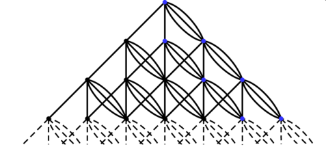
We may assume that δ<knn⁡(x)<δ​d\delta<\frac{k_{n}}{n(x)}<\delta d for some δ>0\delta>0. First, we suppose that some typical n=n⁡(x)>>mn=n(x)>>m and knk_{n} are taken. We consider a set of ingoing finite paths of length mm to the vertex (n,k),d≤k≤d⁡(n−1),n>>m(n,k),d\leq k\leq d(n-1),n>>m. Self-similarity of BpB_{p} implies that these paths can be considered as paths going from the origin to some vertex (m,j),0≤j≤m​d,(m,j),0\leq j\leq md, of BpB_{p}, see Fig. 4. As shown in Section 3.33.3 above, each such path correspond to a point from Gqm,G_{q}^{m}, which in its turn correspond to qq-rr-adic interval of rank mm. Let xm,j,0⩽j⩽m​dx_{m,j},0\leqslant j\leqslant md denote length of such interval and ym,jy_{m,j}, denote increment of the function ψnM\psi_{n}^{M} on the interval (m,j)(m,j). Values (xm,j,ym,j)(x_{m,j},y_{m,j}) may be defined inductively: For m=0m=0 by x0,0=1,y0,0=0x_{0,0}=1,y_{0,0}=0, and for m>0m>0 and indices jj such that (m−1)​d<j⩽m​d(m-1)d<j\leqslant md by xm,j=∑i=0jai​Cp​(n−m,n​d−k+j−d​i)Hn,k,ym,j=ψnM​(xm,j)x_{m,j}=\sum\limits_{i=0}^{j}\frac{a_{i}C_{p}(n-m,nd-k+j-di)}{H_{n,k}},\,y_{m,j}=\psi_{n}^{M}(x_{m,j}); for other values of jj by recursive expression xm−1,i=∑j=0daj​xm,i−j,x_{m-1,i}=\sum_{j=0}^{d}a_{j}x_{m,i-j}, ym−1,i=∑j=0daj​ym,i−j.y_{m-1,i}=\sum_{j=0}^{d}a_{j}y_{m,i-j}. Therefore function ψnjM\psi_{n_{j}}^{M} is totally defined by its values at xm,jx_{m,j}, 1⩽m⩽M,1\leqslant m\leqslant M, (m−1)​d<j⩽m​d(m-1)d<j\leqslant md. Going to the limit we obtain the claim. ∎
Refer to caption
Figure 4: For Bratteli diagram BpB_{p} and graph of ingoing paths.

Stochastic version of Theorem 7 is obtained from the following claim: for any ε>0\varepsilon>0 for μq\mu_{q}-a.e. xx there exists subsequence nj​(x)n_{j}(x) such that Num​(wj),wj=(x1,…​xnj),\text{Num}(w^{j}),w^{j}=(x_{1},\dots x_{n_{j}}), satisfies the following condition Num​(wj)Hnj,knj<ε.\frac{\text{Num}(w^{j})}{H_{n_{j},k_{n_{j}}}}<\varepsilon. In fact, even more strong result holds. It follows from the recurrence property of one-dimensional random walk and was first proved by É. Janvresse and T. de la Rue in [15] to show that the Pascal adic transformation is loosely Bernoulli. Later it was generalized in [19, 12] for the polynomial adic systems.

Lemma 3.

For any ε>0\varepsilon>0 and μq×μq\mu_{q}\times\mu_{q}-a.e. pair of paths (x,y)∈X×X(x,y)\in X\times X there is a subsequence njn_{j} such that knj​(x)=knj​(y)k_{n_{j}}(x)=k_{n_{j}}(y) and indices Num​(ωx)\text{\emph{Num}}(\omega_{x}), Num​(ωy)\text{\emph{Num}}(\omega_{y}) of paths ωx=(x1,x2,…​xnj)\omega_{x}=(x_{1},x_{2},\dots x_{n_{j}}) and ωy=(y1,y2,…​ynj)\omega_{y}=(y_{1},y_{2},\dots y_{n_{j}}) satisfy the following inequlity Num​(ωz)/Hnj,knj​(x)<ε,\text{\emph{Num}}(\omega_{z})/H_{n_{j},k_{n_{j}}(x)}<~\varepsilon, z∈{x,y},z\in\{x,y\}, for each j∈ℕj\in\mathbb{N}.

Theorem 8.

(Stochastic variant of Theorem 7.) Let (X,T,μq),(X,T,\mu_{q}), q∈(0,1a0),q\in(0,\frac{1}{a_{0}}), and gg be a cylindric function from ℱN\mathscr{F}_{N}. Then for μq\mu_{q}-a.e. xx limiting curve φxg∈C⁡[0,1]\varphi^{g}_{x}\in C[0,1] exists if and only if function gg is not cohomologous to a constant.

Proof.

Follows from Lemma 3, Theorem 7 and Theorem 2. ∎

Remark Lemma 3 implies that appropriate choice of stabilizing sequence ln​(x)l_{n}(x) can provide the same limiting curve φxg,\varphi_{x}^{g}, limj→∞‖φx,lj​(x)g−φxg‖=0\lim\limits_{j\rightarrow\infty}||\varphi_{x,l_{j}(x)}^{g}-\varphi_{x}^{g}||=0, for μq\mu_{q}-a.e. xx.

Finally we prove Proposition 2 used above. It generalizes Proposition 3.13.1 from [16]. However, its proof needs an additional statement due to the non unimodality of generalized binomial coefficients Cp​(n,k)C_{p}(n,k):

Lemma 4.

Let p⁡(x)=a0+a1​x+⋯+ad​xdp(x)=a_{0}+a_{1}x+\dots+a_{d}x^{d} be a positive integer polynomial. Then the following holds:

1.1. There exist n1∈ℕn_{1}\in\mathbb{N} and C1>0C_{1}>0, depending only on {a0,…,ad}\{a_{0},\dots,a_{d}\}, such that maxk⁡{Cp​(n,k+1)Cp​(n,k),Cp​(n,k)Cp​(n,k+1)}⩽C1​n\max\limits_{k}\{\frac{C_{p}(n,k+1)}{C_{p}(n,k)},\frac{C_{p}(n,k)}{C_{p}(n,k+1)}\}\leqslant C_{1}n for n>n1.n>n_{1}.

2.2. Cp​(n−1,k−i)⩽1ai​max⁡{kn,1−kn}​Cp​(n,k), 0⩽i⩽d.C_{p}(n-1,k-i)\leqslant\frac{1}{a_{i}}\max\{\frac{k}{n},1-\frac{k}{n}\}C_{p}(n,k),\,0\leqslant i\leqslant d.

Proof.

1.1. Let XX be a discrete random variable on {0,1,…,d}\{0,1,\dots,d\} with distribution associated to the polynomial p⁡(x),p(x), that is Prob​(X=k)=ak/p⁡(1),0⩽k⩽d.\text{Prob}(X=k)=a_{k}/{p(1)},0\leqslant k\leqslant d. Distribution of a sum Yn=X1+X2+…​XnY_{n}=X_{1}+X_{2}+\dots X_{n} of i.i.d. random variables Xk,0⩽k⩽n,X_{k},0\leqslant k\leqslant n, with distributions associated to the polynomial p⁡(x)p(x), is associated to the polynomial pn​(x),p^{n}(x), i.e. Prob​(Yn=k)=Cp​(n,k)/pn​(1),0⩽k⩽n​d.\text{Prob}(Y_{n}=k)=C_{p}(n,k)/{p^{n}(1)},0\leqslant k\leqslant nd. A. Oldyzko and L. Richmond showed in [21] that the function fn​(k)≡Prob​(Yn=k)f_{n}(k)\equiv\text{Prob}(Y_{n}=k) is asymptotically unimodal, i.e. for n≥n1n\geq n_{1}, coefficients Cp​(n,k),C_{p}(n,k), 0⩽k⩽n​d,n⩾n1,0\leqslant k\leqslant nd,n\geqslant n_{1}, first increase (in kk) and decrease then.

We denote by CC and cc the maximum and the minimum values of the coefficients {Cp​(n1,k)}k=0n1​d\{C_{p}(n_{1},k)\}_{k=0}^{n_{1}d} of the polynomial pn1​(x)p^{n_{1}}(x). Let also amaxa_{\max} denote the maximum of the coefficients {a0,…,ad}\{a_{0},\dots,a_{d}\} of the polynomial p⁡(x)p(x). We will use induction in nn to prove that Cp​(n,k+1)Cp​(n,k)⩽amax​Cc​d​n,0⩽k⩽n​d−1,n⩾n1\frac{C_{p}(n,k+1)}{C_{p}(n,k)}\leqslant a_{\max}\frac{C}{c}dn,0\leqslant k\leqslant nd-1,n\geqslant n_{1}. (The second estimate Cp​(n,k)Cp​(n,k+1)⩽amax​Cc​d​n\frac{C_{p}(n,k)}{C_{p}(n,k+1)}\leqslant a_{\max}\frac{C}{c}dn can be proved in the same way). We start now with the base case: For n=n1n=n_{1} it obviously holds that Cp​(n1,k+1)Cp​(n1,k)⩽Cc⩽C​d​amaxc,0⩽k⩽n,\frac{C_{p}(n_{1},k+1)}{C_{p}(n_{1},k)}\leqslant\frac{C}{c}\leqslant\frac{Cda_{\max}}{c},0\leqslant k\leqslant n, hence we have shown the base case.

Now assume that we have already shown Cp​(n−1,k)Cp​(n−1,k−1)⩽C​d​amaxc​(n−1)\frac{C_{p}(n-1,k)}{C_{p}(n-1,k-1)}\leqslant\frac{Cda_{\max}}{c}(n-1), where 1⩽k⩽d⁡(n−1)1\leqslant k\leqslant d(n-1) and n≥n1.n\geq n_{1}. We need to show that Cp​(n,k)Cp​(n,k−1)⩽C​d​amaxc​n,\frac{C_{p}(n,k)}{C_{p}(n,k-1)}\leqslant\frac{Cda_{\max}}{c}n, 1⩽k⩽d​n.1\leqslant k\leqslant dn.

Cp​(n,k+1)Cp​(n,k)=∑i=0dai​Cp​(n−1,k+1−i)∑i=0dai​Cp​(n−1,k−i)⩽⩽Cp​(n−1,k)​(a0+a1+⋯+ad−1+d​amax​ad​Cc​(n−1))ad​Cp​(n−1,k)⩽⩽a0+a1+⋯+ad−1−d​amaxad+amax​C​d​nc⩽amax​C​dc​n.\frac{C_{p}(n,k+1)}{C_{p}(n,k)}=\frac{\sum_{i=0}^{d}a_{i}C_{p}(n-1,k+1-i)}{\sum_{i=0}^{d}a_{i}C_{p}(n-1,k-i)}\leqslant\\ \leqslant\frac{C_{p}(n-1,k)\big(a_{0}+a_{1}+\dots+a_{d-1}+da_{\max}a_{d}\frac{C}{c}(n-1)\big)}{a_{d}C_{p}(n-1,k)}\leqslant\\ \leqslant\frac{a_{0}+a_{1}+\dots+a_{d-1}-da_{\max}}{a_{d}}+\frac{a_{\max}Cdn}{c}\leqslant\frac{a_{\max}Cd}{c}n. (8)

2.2. The statement follows directly from the following identity for the generalized binomial coefficients:

∑i=1dCp​(n−1,k−i)​ai​i=kn​Cp​(n,k).\sum\limits_{i=1}^{d}C_{p}(n-1,k-i)a_{i}i=\frac{k}{n}C_{p}(n,k). (9)

To show it we differentiate identity pn​(x)=∑k≥0Cp​(n,k)​xkp^{n}(x)=\sum_{k\geq 0}C_{p}(n,k)x^{k} resulting n​pn−1​(x)​p′​(x)=∑k≥0k​Cp​(n,k)​xk−1,np^{n-1}(x)p^{\prime}(x)=\sum_{k\geq 0}kC_{p}(n,k)x^{k-1}, p′​(x)=a1+2​a2​x+⋯+d​ad​xd−1.p^{\prime}(x)=a_{1}+2a_{2}x+\dots+da_{d}x^{d-1}. It remains to equate exponents from the two sides. ∎

The following proposition generalizes Propositon 3.1 from [16]. We preserved the original notation where it was possible.

Proposition 2.

Let N⩾1N\geqslant 1 be a positive integer and δ∈(0,14)\delta\in(0,\frac{1}{4}) be a small parameter. Let A=A⁡(n¯,k¯)∈Bp{A}=A(\bar{n},\bar{k})\in B_{p} be a vertex with coordinates (n¯,k¯)\big(\bar{n},\bar{k}\big) satisfying 2​δ​n¯⩽k⩽(d−2​δ)​n¯2\delta\bar{n}\leqslant k\leqslant(d-2\delta)\bar{n} and 2​δ​n¯⩽n​d−k⩽(d−2​δ)​n¯2\delta\bar{n}\leqslant nd-k\leqslant(d-2\delta)\bar{n}. Let αl,0⩽l⩽N​d,\alpha_{l},0\leqslant l\leqslant Nd, be real numbers, such that ∑l=0N​dαl2>0\sum\limits_{l=0}^{Nd}\alpha_{l}^{2}>0. Let n,N⩽n⩽n¯,n,N\leqslant n\leqslant\bar{n}, and B⁡(n,k)=(n,k){B}(n,k)=\big(n,k\big) be a vertex with coordinates satisfying 0⩽k⩽k¯,0⩽n−k⩽n¯−k¯.0\leqslant k\leqslant\bar{k},0\leqslant n-k\leqslant\bar{n}-\bar{k}. Define

γn,k=1R​∑l=0N​dαl​Cd​(n−N,k−l),\gamma_{n,k}=\frac{1}{R}\sum\limits_{l=0}^{Nd}\alpha_{l}\,C_{d}(n-N,k-l), (10)

where R=R⁡(A,B,δ)R=R(A,B,\delta) is a renormalization constant such that |γn,k||\gamma_{n,k}| are uniformly in nn and kk from 0⩽k⩽k¯,0⩽n−k⩽n¯−k¯,N⩽n⩽n¯0\leqslant k\leqslant\bar{k},0\leqslant n-k\leqslant\bar{n}-\bar{k},N\leqslant n\leqslant\bar{n} bounded by 22. Then there exist a constant C=C⁡(δ,N),C=C(\delta,N), such that, provided n¯\bar{n} is large enough, the following inequality holds for all n,kn,k:

|γn,k|⩽3​e−C⁡(n¯−n).|\gamma_{n,k}|\leqslant 3e^{-C(\bar{n}-n)}.

Conditions on the vertex A{A} δ\delta-separate it from "boundary"  vertices (n¯,0)(\bar{n},0) and (n¯,d​n¯)(\bar{n},d\bar{n}). Conditions on the vertex B=B⁡(n,k)B={B}(n,k) provides it can be considered as a vertex in a "flipped"  graph and that it can be connected with the vertex AA, see Fig. 5.

Figure 5: Vertices AA and BB in the graph BpB_{p}.
Proof.

We can assume that n¯>2​n1,\bar{n}>2n_{1}, where n1=n1​(a0,a1,…,ad)n_{1}=n_{1}(a_{0},a_{1},\dots,a_{d}), is defined in the proof of Lemma 4. Let l0,0⩽l0⩽N​d,l_{0},0\leqslant l_{0}\leqslant Nd, be such that coefficient αl0\alpha_{l_{0}} is nonzero. We can rewrite the right hand side of (10) as follows:

R​γn,k=Cd​(n−N,k−l0)​P​(n,k,l0),N⩽n⩽n¯,0⩽k⩽n​d,R\gamma_{n,k}=C_{d}(n-N,k-l_{0})P(n,k,l_{0}),N\leqslant n\leqslant\bar{n},0\leqslant k\leqslant nd,

where P⁡(n,k,l0)P(n,k,l_{0}) is defined by ∑l=0Nαl​Cd​(n−N,k−l)Cd​(n−N,k−l0)\sum\limits_{l=0}^{N}\alpha_{l}\,\frac{C_{d}(n-N,k-l)}{C_{d}(n-N,k-l_{0})}. Let α\alpha denote the maximum of |αl|,0⩽l⩽N​d.|\alpha_{l}|,0\leqslant l\leqslant Nd. We want to show that there is a polynomial Q⁡(x)Q(x) of degree deg​(Q)≤N​d\text{deg}(Q)\leq Nd such that

|P⁡(n,k,l0)−P⁡(n¯,k¯,l0)|⩽Q⁡(n¯).|P(n,k,l_{0})-P(\bar{n},\bar{k},l_{0})|\leqslant Q(\bar{n}). (11)

It is enough to show that there is c1>0c_{1}>0 such that |Cd​(n−N,k−l)Cd​(n−N,k−l0)|⩽c1​nN​d,0⩽l⩽N​d,N⩽n⩽n¯|\frac{C_{d}(n-N,k-l)}{C_{d}(n-N,k-l_{0})}|\leqslant c_{1}n^{Nd},0\leqslant l\leqslant Nd,N\leqslant n\leqslant\bar{n}. The latter inequality follows from N​dNd fold application of part 11 of Lemma 4. Define function Q~\tilde{Q} by Q~=P⁡(n,k,l0)−P⁡(n¯,k¯,l0)\tilde{Q}=P(n,k,l_{0})-P(\bar{n},\bar{k},l_{0}). We can write

γn,k=1R​Cd​(n−N,k−l0)​P​(n,k,l0)==Cd​(n−N,k−l0)Cd​(n¯−N,k¯−l0)​Cd​(n¯−N,k¯−l0)​P​(n,k,l0)R==Cd​(n−N,k−l0)Cd​(n¯−N,k¯−l0)​Cd​(n¯−N,k¯−l0)​(P⁡(n¯,k¯,l0)+Q~)R.\gamma_{n,k}=\frac{1}{R}C_{d}(n-N,k-l_{0})P(n,k,l_{0})=\\ =\frac{C_{d}(n-N,k-l_{0})}{C_{d}(\bar{n}-N,\bar{k}-l_{0})}\frac{C_{d}(\bar{n}-N,\bar{k}-l_{0})P(n,k,l_{0})}{R}=\\ =\frac{C_{d}(n-N,k-l_{0})}{C_{d}(\bar{n}-N,\bar{k}-l_{0})}\frac{C_{d}(\bar{n}-N,\bar{k}-l_{0})(P(\bar{n},\bar{k},l_{0})+\tilde{Q})}{R}. (12)

By the assumption we have |γn¯,k¯|=|1R​P​(n¯,k¯,l0)​Cd​(n¯−N,k¯−l0)|⩽2.|\gamma_{\bar{n},\bar{k}}|=|\frac{1}{R}P(\bar{n},\bar{k},l_{0})C_{d}(\bar{n}-N,\bar{k}-l_{0})|\leqslant 2. Therefore inequality (11) can be written as |Q~|⩽Q.|\tilde{Q}|\leqslant Q. We get

|γn,k|⩽3​Q⁡(n¯)​Cd​(n−N,k−l0)Cd​(n¯−N,k¯−l0).|\gamma_{n,k}|\leqslant 3\frac{Q(\bar{n})C_{d}(n-N,k-l_{0})}{C_{d}(\bar{n}-N,\bar{k}-l_{0})}.

Applying the estimate from part 22 of Lemma 4 (n¯−n)(\bar{n}-n) times and using assumptions on the vertices AA and BB, we obtain that Cd​(n−N,k−l0)Cd​(n¯−N,k¯−l0)⩽3​e−C~​(δ)​(n¯−n)\frac{C_{d}(n-N,k-l_{0})}{C_{d}(\bar{n}-N,\bar{k}-l_{0})}\leqslant 3e^{-\tilde{C}(\delta)(\bar{n}-n)} for some C~​(δ)>0.\tilde{C}(\delta)>0. Finally we get (an independent of the initial choice of l0l_{0}) estimate:

|γn,k|⩽3​Q⁡(n¯)​Cd​(n−N,k−l0)Cd​(n¯−N,k¯−l0)⩽3​e−C​(δ)​(n¯−n)|\gamma_{n,k}|\leqslant 3\frac{Q(\bar{n})C_{d}(n-N,k-l_{0})}{C_{d}(\bar{n}-N,\bar{k}-l_{0})}\leqslant 3e^{-C(\delta)(\bar{n}-n)}

for some C⁡(δ)>0.C(\delta)>0.

∎

3.5 Examples of limiting curves

Let q1q_{1} and q2q_{2} be two numbers (parameters) from (0,1).(0,1). We consider the function Sq1,q2p:[0,1]→[0,1]S^{p}_{q_{1},q_{2}}:[0,1]\rightarrow[0,1] that maps a number xx with q1q_{1}-rr-adic representation x=∑j=1∞Iq1​(ωj)​q1j​(tq1q1)a¯1⋅s¯j+2​a¯2⋅s¯j+⋯+d​a¯d⋅s¯jx=\sum\limits_{j=1}^{\infty}I_{q_{1}}(\omega_{j})q_{1}^{j}\Big(\frac{t_{q_{1}}}{{q_{1}}}\Big)^{\bar{a}_{1}\cdot\bar{s}_{j}+2\bar{a}_{2}\cdot\bar{s}_{j}+\dots+d\,\bar{a}_{d}\cdot\bar{s}_{j}} to

Sq1,q2p​(x)=∑j=1∞Iq2​(ωj)​q2j​(tq2q2)a¯1⋅s¯j+2​a¯2⋅s¯j+⋯+d​a¯d⋅s¯j.S^{p}_{q_{1},q_{2}}(x)=\sum\limits_{j=1}^{\infty}I_{q_{2}}(\omega_{j})q_{2}^{j}\Big(\frac{t_{q_{2}}}{{q_{2}}}\Big)^{\bar{a}_{1}\cdot\bar{s}_{j}+2\bar{a}_{2}\cdot\bar{s}_{j}+\dots+d\,\bar{a}_{d}\cdot\bar{s}_{j}}. (13)

For any q1q_{1}-rr-stationary point x0=∑j=1mIq1​(ωj)​q1j​(tq1q1)a¯1⋅s¯j+2​a¯2⋅s¯j+⋯+d​a¯d⋅s¯jx_{0}=\sum\limits_{j=1}^{m}I_{q_{1}}(\omega_{j})q_{1}^{j}\Big(\frac{t_{q_{1}}}{{q_{1}}}\Big)^{\bar{a}_{1}\cdot\bar{s}_{j}+2\bar{a}_{2}\cdot\bar{s}_{j}+\dots+d\,\bar{a}_{d}\cdot\bar{s}_{j}} and any x∈[0,1]x\in[0,1] the function Sq1,q2pS^{p}_{q_{1},q_{2}} satisfies the following self-affinity property:

Sq1,q2p​(x0+rq1​x)=Sq1,q2p​(x0)+rq2​Sq1,q2p​(x),S^{p}_{q_{1},q_{2}}\Big(x_{0}+r_{q_{1}}x\Big)=S^{p}_{q_{1},q_{2}}(x_{0})+r_{q_{2}}S^{p}_{q_{1},q_{2}}(x), (14)

where rqi=qim(tqiqi)a¯1⋅s¯m+2​a¯2⋅s¯m+⋯+d​a¯d⋅s¯m,i=1,2.r_{q_{i}}=q_{i}^{m}\Big(\frac{t_{q_{i}}}{{q_{i}}}\Big)^{\bar{a}_{1}\cdot\bar{s}_{m}+2\bar{a}_{2}\cdot\bar{s}_{m}+\dots+d\,\bar{a}_{d}\cdot\bar{s}_{m}},i=1,2. Expression (14) means that the graph of Sq1,q2pS^{p}_{q_{1},q_{2}} considered on the qq-rr-adic interval [x0,x0+rq1][x_{0},x_{0}+r_{q_{1}}] coincides after renormalization with the graph of Sq1,q2pS^{p}_{q_{1},q_{2}} on the whole interval [0,1][0,1]. Also for q1=1/rq_{1}=1/r function S1/r,q2pS^{p}_{1/r,q_{2}} is the distribution function of the measure μ~q2.\tilde{\mu}_{q_{2}}.

Functions Sq1,q2p​(⋅)S^{p}_{q_{1},q_{2}}(\cdot) allow us to define new functions

𝒯p,q1k:=∂kSq1,q2p∂q2k|q2=q1,k∈ℕ.\mathcal{T}_{p,q_{1}}^{k}:=\frac{\partial^{k}S^{p}_{q_{1},q_{2}}}{\partial q_{2}^{k}}\Big|_{q_{2}=q_{1}},\ k\in\mathbb{N}.

If k=0k=0 we will assume that 𝒯p,q0​(x)=x.\mathcal{T}_{p,q}^{0}(x)=x. For q=1/2q={1/2} and k=1k=1 function 12​𝒯1+x,1/21\frac{1}{2}\mathcal{T}_{1+x,{1/2}}^{1} is the Takagi function, see [22]. The function 𝒯p,q1k\mathcal{T}_{p,q_{1}}^{k} on the interval [x0,x0+rq1][x_{0},x_{0}+r_{q_{1}}] can be expressed by a linear combination of the functions 𝒯p,q1j,0⩽j⩽k.\mathcal{T}_{p,q_{1}}^{j},0\leqslant j\leqslant k. (Expression can be easily obtained by differentiating identity (14) with respect to parameter q2q_{2} and defining q2q_{2} equal to q1q_{1}.)

Refer to caption
Figure 6: Graph of the funciton 𝒯p,q1\mathcal{T}_{p,q}^{1}, defined by polynomial p⁡(x)=1+x+2​x2p(x)=1+x+2x^{2} with parameter qq equal to 14.\frac{1}{4}.
Theorem 9.

Functions 𝒯p,qk,q∈(0,1/a0),k≥1,\mathcal{T}_{p,q}^{k},q\in(0,1/a_{0}),k\geq 1, are continuous functions on [0,1][0,1].

Proof.

The proof is based on the fact that any two points xx and yy from the same qq-rr-adic interval of rank mm have the same coordinates (ω1,ω2,…,ωm)(\omega_{1},\omega_{2},\dots,\omega_{m}) in qq-rr-adic expansion. This provides a straightforward estimate for the difference |𝒯p,q1​(x)−𝒯p,q1​(y)||\mathcal{T}_{p,q}^{1}(x)-\mathcal{T}_{p,q}^{1}(y)|.

Let b=bqb=b_{q} denote the ratio tq/qt_{q}/q. As shown in Section 3.33.3 above any xx in (0,1)(0,1) can be coded by a path ω=(ωi)i=1∞,ωi∈{0,1​…,r−1}=𝒜,\omega=(\omega_{i})_{i=1}^{\infty},\omega_{i}\in\{0,1\dots,r-1\}=\mathcal{A}, in rr-adic (perfectly balanced) tree ℳr\mathcal{M}_{r}. The function 𝒯p,q1\mathcal{T}_{p,q}^{1} maps x=xq∈[0,1]x=x_{q}\in[0,1] with qq-rr adic series representation

x=∑j=1∞(∑i=0ωj−1bi)​qj​ba¯1⋅s¯j+2​a¯2⋅s¯j+⋯+d​a¯d⋅s¯j,x=\sum\limits_{j=1}^{\infty}\Big(\sum\limits_{i=0}^{\omega_{j}-1}b^{i}\Big)q^{j}b^{\bar{a}_{1}\cdot\bar{s}_{j}+2\bar{a}_{2}\cdot\bar{s}_{j}+\dots+d\,\bar{a}_{d}\cdot\bar{s}_{j}},

to z=∂∂q​xq.z=\frac{\partial}{\partial q}x_{q}. Let s~j\tilde{s}_{j} denote the sum a¯1⋅s¯j+2​a¯2⋅s¯j+⋯+d​a¯d⋅s¯j\bar{a}_{1}\cdot\bar{s}_{j}+2\bar{a}_{2}\cdot\bar{s}_{j}+\dots+d\,\bar{a}_{d}\cdot\bar{s}_{j}.

Derivative ∂∂q​(qj​bl)\frac{\partial}{\partial q}(q^{j}b^{l}) equals to qj−1​bl−1​[(j−l)​b+l​tq′],q^{j-1}b^{l-1}[(j-l)b+lt^{\prime}_{q}], where l=s~j−ωj+i.l=\tilde{s}_{j}-\omega_{j}+i. Using implicit function theorem we find that

tq′=−a0​d​qd−1+a1​(d−1)​qd−2​tq+⋯+ad−1​tqd−1−(d−1)​qd−2a1​qd−1+2​a2​qd−2​tq+…​ad​tqd−1​d.t^{\prime}_{q}=-\frac{a_{0}dq^{d-1}+a_{1}(d-1)q^{d-2}t_{q}+\dots+a_{d-1}t_{q}^{d-1}-(d-1)q^{d-2}}{a_{1}q^{d-1}+2a_{2}q^{d-2}t_{q}+\dots a_{d}t_{q}^{d-1}d}. (15)

Let also amaxa_{\max} denote the maximum of the coefficients {a0,…,ad}\{a_{0},\dots,a_{d}\} of the polynomial p⁡(x)p(x). We have |tq′|≤amax​2​d2q.|t^{\prime}_{q}|\leq a_{\max}\frac{2d^{2}}{q}. Let pm​a​x∈(0,1)p_{max}\in(0,1) denote the maximum of {q,tq,tq2q,…,tqdqd−1}.\{q,t_{q},\frac{t_{q}^{2}}{q},\dots,\frac{t_{q}^{d}}{q^{d-1}}\}.

Assume yy is the left boundary of some qq-rr-adic interval of rank m,m, containing point xx. Then the following inequality holds (we simply write TT for Tp,q1T_{p,q}^{1}):

|T⁡(y)−T⁡(x)|≤∑j=m∞∑i=0ωj−1|∂∂q​(qj​bs~j+i)|.|T(y)-T(x)|\leq\sum\limits_{j=m}^{\infty}\sum\limits_{i=0}^{\omega_{j}-1}\big|\frac{\partial}{\partial q}\big(q^{j}b^{\tilde{s}_{j}+i}\big)\big|.

Using estimate |qj​bs~j+i|≤(pm​a​x)j|q^{j}b^{\tilde{s}_{j}+i}|\leq(p_{max})^{j}, 0≤i≤r−10\leq i\leq r-1, we see that the absolute value of ∂∂q​(qj​bl)\frac{\partial}{\partial q}(q^{j}b^{l}) for j>2j>2 is estimated by expression P⁡(j,q)​(pm​a​x)j−2P(j,q)(p_{max})^{j-2}, where P⁡(j,q)P(j,q) is some polynomial. Define ε\varepsilon to be equal to 0.99.0.99. Then for mm large enough it holds:

|T⁡(y)−T⁡(x)|≤∑j=m∞∑i=0ωj−1P⁡(j,q)​(pm​a​x)j−2≤C​(pm​a​x)m​ε,|T(y)-T(x)|\leq\sum\limits_{j=m}^{\infty}\sum\limits_{i=0}^{\omega_{j}-1}P(j,q)(p_{max})^{j-2}\leq C(p_{max})^{m\varepsilon}, (16)

where CC is some constant.

In general case we can assume that points xx and x+δx+\delta are from some qq-rr-adic interval of rank m=m⁡(δ),limδ→0m⁡(δ)=+∞,m=m(\delta),\lim\limits_{\delta\rightarrow 0}m(\delta)=+\infty, and let yy be the left boundary point of this interval. Then

|T⁡(x+δ)−T⁡(x)|≤|T⁡(y)−T⁡(x)|+|T⁡(y)−T⁡(x+δ)|≤2​C​pm​a​xm​ε|T(x+\delta)-T(x)|\leq|T(y)-T(x)|+|T(y)-T(x+\delta)|\leq 2Cp_{max}^{m\varepsilon}

For k>1k>1 we can use a similar argument based on the following estimate for the kk-th derivative: |∂k∂qk​qj​bl|≤Pk​(j,q)​(pm​a​x)j−k−1,|\frac{\partial^{k}}{\partial q^{k}}q^{j}b^{l}|\leq P_{k}(j,q)(p_{max})^{j-k-1}, where j>kj>k and Pk​(j,q)P_{k}(j,q) is some polynomial. ∎

Proposition 3.

For a cylindrical function g=−∑j=0djaj𝟙{k1(x1)=j}∈ℱ1g=-\sum_{j=0}^{d}ja_{j}\mathbbm{1}_{\{k^{1}(x_{1})=j\}}\in\mathscr{F}_{1} and for μq\mu_{{q}}-a.e. xx there is a stabilizing sequence ln​(x)l_{n}(x) such that the limiting function is 𝒯p,q1\mathcal{T}_{p,q}^{1}.

Proof.

For simplicity we will present the proof for p⁡(x)=1+x+x2.p(x)=1+x+x^{2}. The general case follows the same steps. Theorem 7 implies that we can find the limiting function φ⁡(x)\varphi(x) as limn→∞φn,k\lim\limits_{n\rightarrow\infty}\varphi_{n,k}, where (by the law of large numbers) knn→𝔼μq​k1\frac{k_{n}}{n}\rightarrow\mathbb{E}_{\mu_{q}}k_{1}. Lemma 2 imply that it is sufficient to show that the function φ⁡(x)\varphi(x) coincide with 𝒯p,q1\mathcal{T}_{p,q}^{1} at x=qjx=q^{j} and x=qj−1​(q+tq)x=q^{j-1}(q+t_{q}), where j∈ℕj\in\mathbb{N}.

The function 𝒯p,q11\mathcal{T}_{p,q_{1}}^{1} maps point x=qjx=q^{j} to ∂∂q​qj=j​qj−1\frac{\partial}{\partial q}q^{j}=jq^{j-1} and point x=qj−1​(q+tq)x=q^{j-1}(q+t_{q}) to qj−2​(j​q+(j−1)​tq+tq′​q)q^{j-2}\big(jq+(j-1)t_{q}+t^{\prime}_{q}q\big). Using expression (15) we see that tq′=1−(2​q+tq)2​tq+q.t^{\prime}_{q}=\frac{1-(2q+t_{q})}{2t_{q}+q}.

Identity (9) implies that hn,kg=kn​Hn,k.h_{n,k}^{g}=\frac{k}{n}H_{n,k}. We need to find the following limits for i∈ℕ,i\in\mathbb{N}, n→∞n\rightarrow\infty and knn→𝔼μq​k1=2​q+tq\frac{k_{n}}{n}\rightarrow\mathbb{E}_{\mu_{q}}k_{1}=2q+t_{q} (we write FF for Fn,kF_{n,k}):

  1. 1.

    lim1Rn​(F⁡(Hn−i,k−2​i)−Hn−i,k−2​iHn,k​F​(Hn,k))\lim\frac{1}{R_{n}}\Big(F(H_{n-i,k-2i})-\frac{H_{n-i,k-2i}}{H_{n,k}}F(H_{n,k})\Big)

  2. 2.

    lim1Rn​(F⁡(Hn−i,k−2​i+Hn−i,k−2​i+1)−Hn−i,k−2​i+Hn−i,k−2​i+1Hn,k​F​(Hn,k))\lim\frac{1}{R_{n}}\Big(F(H_{n-i,k-2i}+H_{n-i,k-2i+1})-\frac{H_{n-i,k-2i}+H_{n-i,k-2i+1}}{H_{n,k}}F(H_{n,k})\Big)

We define the normalizing coefficient RnR_{n} by Rn=q​Hn,kn​(2−𝔼μq​k1)R_{n}=\frac{qH_{n,k}}{n}(2-\mathbb{E}_{\mu_{q}}k_{1}). After some computations we see that the first limit equals i​qi−1,iq^{i-1}, and the second to qi−2​(i​q+(i−1)​tq+tq′​q)q^{i-2}\big(iq+(i-1)t_{q}+t^{\prime}_{q}q\big). These shows that that the limiting function φ\varphi coincides with the function 𝒯p,q11\mathcal{T}_{p,q_{1}}^{1} on a dense set of qq-22-stationary points. Therefore, by Theorem 9 these functions coincide.

∎

Numerical simulations show that limiting functions 𝒯p,qk,k⩾1,\mathcal{T}_{p,q}^{k},k\geqslant 1, and their linear combinations arise as limiting functions limn→∞φn,kng\lim\limits_{n\rightarrow\infty}\varphi_{n,k_{n}}^{g} for a general cylindrical function g∈ℱNg\in\mathcal{F}_{N}. We do not have any proof of this statement except for the case of the Pascal adic, see Theorem 3 above. Expression (3) shows that for a cylindrical function g∈ℱNg\in\mathscr{F}_{N} the partial sum Fn,kgF^{g}_{n,k} is defined by the coefficients hN,kg,0≤k≤N​d.h_{N,k}^{g},0\leq k\leq Nd. Its seems to be useful to define hN,kgmh_{N,k}^{g_{m}} by the generating function hN,kgm=coeff​[vm]​(h0+h1​v+⋯+hd​vd)k​p​(v)N​d−k,h_{N,k}^{g_{m}}=\text{coeff}[v^{m}]\,(h_{0}+h_{1}v+\dots+h_{d}v^{d})^{k}p(v)^{Nd-k}, where functions gmg_{m} forms an orthogonal basis. (For the Pascal adic the function (1−a​v)k​(1+v)n−k,a=1−qq,(1-av)^{k}(1+v)^{n-k},a=\frac{1-q}{q}, is the generating function of the Krawtchouk polynomials and the basis gmg_{m} is the basis of Walsh functions, see [11]).

4 Limit of limiting curves

In this section we answer the question by É. Janvresse, T. de la Rue and Y. Velenik from [16], page 20, Section 4.3.1.

Refer to caption
Refer to caption
Refer to caption
Refer to caption
Figure 7: Limiting curves observed for the polynomial adic transformations (from left to right): d+1=2,3,8,32.d+1=2,3,8,32.

Let q∈(0,1)q\in(0,1) and tq∈(0,1)t_{q}\in(0,1) be the unique solution in (0,1)(0,1) of the equation

qd+qd−1​t+⋯+td=qd−1.q^{d}+q^{d-1}t+\dots+t^{d}=q^{d-1}.

As above, we denote by b=bqb=b_{q} the ratio tq/qt_{q}/q. Any xx in (0,1)(0,1) has an almost unique (d+1)(d+1)-adic representation:

x=∑j=1∞(∑i=0ωj−1bi)​qj​bsj1+2​sj2+…​d​sjd−ωj,x=\sum\limits_{j=1}^{\infty}\Big(\sum\limits_{i=0}^{\omega_{j}-1}b^{i}\Big)q^{j}b^{s_{j}^{1}+2s_{j}^{2}+\dots ds_{j}^{d}-\omega_{j}}, (17)

where ω=(ωi)i=1∞,ωi∈{0,1​…,d}=𝒜,\omega=(\omega_{i})_{i=1}^{\infty},\omega_{i}\in\{0,1\dots,d\}=\mathcal{A}, is a path in (d+1)(d+1)-adic (perfectly balanced) tree ℳd+1\mathcal{M}_{d+1} and sjks_{j}^{k} is the number of occurrences of letter kk among (ω1,ω2,…,ωj).(\omega_{1},\omega_{2},\dots,\omega_{j}).

We denote by Sq​(x)S_{q}(x) the (anaclitic in parameter qq) function defined by (a uniformly summable in xx) series (17). We put q∗q_{*} equal to 1/(d+1)1/(d+1) (this is so called symmetric case tq∗=q∗t_{q_{*}}=q_{*}). If d=1d=1 representation (17) for q∗=1/2q^{*}=1/2 is a usual dyadic representation of x∈(0,1)x\in(0,1).

The authors of [16] were interested in the limiting behavior of the graph of the function

𝒯~d:x↦1d+1​∂Sq∂q|q=q∗\tilde{\mathcal{T}}_{d}:x\mapsto\frac{1}{d+1}\frac{\partial S_{q}}{\partial q}\Big|_{q=q_{*}}

for large values of dd (we also introduced vertical normalization by d+1d+1, if d=1d=1 the graph of 12​T1\frac{1}{2}T_{1} is the Takagi curve). On the basis of a series of numerical simulations they noticed that limiting curves for d→∞d\rightarrow\infty seem to converge to a smooth curve. Below we will show that the limiting curve for d=∞d=\infty is actually a parabola, see Fig. 7.

We are going split the unit interval into d+1d+1 subintervals Ii=(id+1;i+1d+1),0≤i≤dI_{i}=(\frac{i}{d+1};\frac{i+1}{d+1}),0\leq i\leq d, of equal length and evaluate the function 𝒯~d\tilde{\mathcal{T}}_{d} at each of the (left) boundary points of these intervals. We also want to show that the function 𝒯~d\tilde{\mathcal{T}}_{d} is uniformly in dd bounded at these intervals. After that we go to the limit in dd.

Symmetry assumption q=tq=q∗q=t_{q}=q_{*} and implicit function theorem (see (15)) imply that tq∗′=−2−dd.t^{\prime}_{q_{*}}=-\frac{2-d}{d}. In its turn this implies bq′=t′q−bqq|q=q∗=−2​(d+1)d.b^{\prime}_{q}=\frac{t^{\prime}}{q}-\frac{b_{q}}{q}\Big|_{q=q_{*}}=-\frac{2(d+1)}{d}. Finally we find that OPEN∂∂q​(qj​br)=j​qj−1​br+r​br−1​qj​bq′|q=q∗=(q∗)j−1​(j+r​q∗​(−2​(d+1)d))=(q∗)j−1​(j−2​rd))\frac{\partial}{\partial q}(q^{j}b^{r})=jq^{j-1}b^{r}+rb^{r-1}q^{j}b^{\prime}_{q}\Big|_{q=q_{*}}=(q_{*})^{j-1}(j+rq_{*}(-\frac{2(d+1)}{d}))=(q_{*})^{j-1}(j-\frac{2r}{d})).

Note that the left boundary point ada_{d} of Ia​d,a∈[0,1],a​d≡[a​d],I_{ad},a\in[0,1],ad\equiv[ad], ([⋅][\,\cdot\,] is an integer part) equals ad=a​dd+1a_{d}=\frac{ad}{d+1} and is coded by the stationary path ω=(ωj)j=1∞∈ℳd+1\omega=(\omega_{j})_{j=1}^{\infty}\in\mathcal{M}_{d+1} with ω1=a​d\omega_{1}=ad and ωj≡0,j≥2.\omega_{j}\equiv 0,j\geq 2.

We have

𝒯~d​(ad)=1d+1​∑i=0d​a−1(j−2​(d​a​(j−1)+i)d)=ad​(1−ad)​d+1d→d→∞ad​(1−ad).\tilde{\mathcal{T}}_{d}(a_{d})=\frac{1}{d+1}\sum\limits_{i=0}^{da-1}\Big(j-\frac{2(da(j-1)+i)}{d}\Big)=a_{d}(1-a_{d})\frac{d+1}{d}\xrightarrow[d\rightarrow\infty]{}a_{d}(1-a_{d}).

This shows that the smooth curve (if exists) should be a parabola.

To complete the proof of the theorem it only remains to show that 𝒯~d​(x)\tilde{\mathcal{T}}_{d}(x) is uniformly bounded in dd at the intervals Ia​dI_{ad}. Analogously to (16) we see that for x∈Ia​dx\in I_{ad} it holds

|𝒯~d​(x)−𝒯~d​(ad)|=1d+1​∑j=2∞q∗j−1​∑i=0ωj−1(j−2​(sj1+2​sj2+⋯+d​sjd−ωj+i)d)≤100​dd+1​∑j=2∞j​q∗j−1≤≤400​d(d+1)2.|\tilde{\mathcal{T}}_{d}(x)-\tilde{\mathcal{T}}_{d}(a_{d})|=\frac{1}{d+1}\sum\limits_{j=2}^{\infty}q_{*}^{j-1}\sum\limits_{i=0}^{\omega_{j}-1}\Big(j-\frac{2(s_{j}^{1}+2s_{j}^{2}+\dots+ds_{j}^{d}-\omega_{j}+i)}{d}\Big)\leq\frac{100d}{d+1}\sum\limits_{j=2}^{\infty}jq_{*}^{j-1}\leq\\ \leq\frac{400d}{(d+1)^{2}}. That finishes our proof.

4.1 Question.

We may heuristically interpret results of Section 44 as existence of a limiting curve of a dynamical system defined by a diagram with "infinite"  number of edges. This leads us to the following questions: Does this system really exist? How to define it correctly? Which properties does it have?

References

  • [1] A. M. Vershik, Uniform algebraic approximations of shift and multiplication operators, Sov. Math. Dokl., 24:3 (1981), 97–100.
  • [2] A. M. Vershik, A theorem on periodical Markov approximation in ergodic theory, J. Sov. Math., 28 (1982), 667–674.
  • [3] A. M. Vershik and A. N. Livshits, Adic models of ergodic transformations, spectral theory, and related topics, Adv. in Soviet Math. AMS Transl., 9, 1992, 185–204.
  • [4] A. M. Vershik, The Pascal automorphism has a continuous spectrum, Funct. Anal. Appl., 45:3 (2011), 173–186.
  • [5] A. M. Vershik, The problem of describing central measures on the path spaces of graded graphs, Funct Anal Its Appl ., 48:4 (2014), 256–271.
  • [6] A. M. Vershik, Several Remarks on Pascal Automorphism and Infinite Ergodic Theory, Armenian Journal of Mathmatics, 7:2 (2015), 85–96.
  • [7] A. G. Kachurovskii, The rate of convergence in ergodic theorems, Russian Mathematical Surveys, 51, 4, (1996) 653–703.
  • [8] I. E.  Manaev, A. R. Minabutdinov, The Kruskal-Katona Function, Conway Sequence, Takagi Curve, and Pascal Adic, Transl: J. Math. Sci.(N.Y.), 196:2 (2014), 192–198.
  • [9] A. R. Minabutdinov, Random Deviations of Ergodic Sums for the Pascal Adic Transformation in the Case of the Lebesgue Measure, Transl: J. Math. Sci.(N.Y.), 209:6, (2015), 953–978.
  • [10] A. R. Minabutdinov, A higher-order asymptotic expansion of the Krawtchouk polynomials, Transl.: J. Math. Sci.(N.Y.) 215:6 (2016), 738–747.
  • [11] A. A. Lodkin,A. R. Minabutdinov, Limiting Curves for the Pascal Adic Transformation, Transl: J. Math. Sci.(N.Y.), 216:1 (2016), 94–119.
  • [12] S. Bailey, Dynamical properties of some non-stationary, non-simple Bratteli-Vershik systems, Ph.D. thesis, University of North Carolina, Chapel Hill, 2006.
  • [13] A. Hajan, Y. Ito, S. Kakutani, Invariant measure and orbits of dissipative transformations, Adv. in Math., 9:1 (1972), 52–65.
  • [14] G. Halasz, Remarks on the remainder in Birkhoff’s ergodic theorem, Acta Mathematica Academiae Scientiarum Hungarica, 28:3-4 (1976), 389–395.
  • [15] É. Janvresse, T. de la Rue, The Pascal adic transformation is loosely Bernoulli, Annales de l’Institut Henri Poincaré (B) Probability and Statistics, 40:2 (2004), 133 – 139.
  • [16] É. Janvresse, T. de la Rue, and Y. Velenik, Self-similar corrections to the ergodic theorem for the Pascal-adic transformation, Stoch. Dyn., 5:1 (2005), 1–25.
  • [17] S. Kakutani, A problem of equidistribution on the unit interval [0, 1], in: Lecture Notes in Math., vol. 541, Springer-Verlag, Berlin, (1976) 369–375.
  • [18] M. Krüppel, De Rham’s singular function, its partial derivatives with respect to the parameter and binary digital sums, Rostocker Math. Kolloq., 64 (2009), 57–74.
  • [19] X. Méla, A class of nonstationary adic transformations, Ann. Inst. H. Poincaré Prob. and Stat., 42:1 (2006), 103–123.
  • [20] X. Méla, K. Petersen, Dynamical properties of the Pascal adic transformation, Ergodic Theory Dynam. Systems, 25:1 (2005), 227–256.
  • [21] A. M. Odlyzko, L. B. Richmond, On the Unimodality of High Convolutions of Discrete Distributions, Ann. Probab., 13 (1985), 299–306.
  • [22] T. Takagi, A simple example of the continuous function without derivative, Proc. Phys.-Math. Soc., 1 (1903), 176–177.