Critical behavior of itinerant fermions - role of finite size effects

Introduction    Critical behavior in itinerant fermionic systems is a fascinating subject, which has attracted much interest in recent years, with particular emphasis on the behavior in two dimensions (2D)[1, 2]. Near a 2D quantum critical point (QCP), soft bosonic fluctuations of the order parameter field mediate strong interaction between low-energy fermions and destroy Fermi-liquid (FL) behavior down to a progressively small energy $\omega_{FL}$, which vanishes at a QCP. Simultaneously, low-energy fermions affect soft bosonic fluctuations by (i) providing Landau damping and (ii) changing the bosonic mass . The destruction of the FL holds even if the overall strength of the interaction is much smaller than the fermionic bandwidth, i.e. when fermions remain itinerant throughout the transition.

Before the feedback from low-energy fermions is included, the inverse propagator of a soft boson is generally assumed to be an analytic function of momentum and frequency: $\chi^{-1}(\bm{\mathrm{q}},\Omega_{m})\propto(|\bm{\mathrm{q}}-\bm{\mathrm{Q}}|^{2}+\Omega^{2}_{m}/c^{2})$, where ${\bf Q}$ is the momentum at which order parameter fluctuations condense at a QCP and $\Omega_{m}$ are Matsubara frequencies. The Landau damping comes from the insertion of the fermionic particle-hole bubble into the bosonic propagator. The form of the Landau damping term depends on whether $\bm{\mathrm{Q}}$ has a finite value (e.g. $(\pi,\pi)$ for a SDW QCP), or is zero, as for a nematic or a ferromagnetic QCP. In the first case the Landau damping term scales as just $|\Omega_{m}|$, while in the second case it scales as $|\Omega_{m}|/q$. In both cases, the Landau damping term wins at small $\Omega_{m}$ over the bare $\Omega^{2}_{m}$ and changes the dynamical exponent from $z=1$ to $z=2$ for $Q\neq 0$ and to $z=3$ for $Q=0$. The one-loop fermionic self-energy due to scattering by Landau overdamped critical fluctuations has a non-FL frequency dependence in 2D: $\Sigma(\omega_{m})\propto\omega^{1-1/z}_{m}$ ($\omega^{1/2}$ at particular hot spots along the Fermi surface (FS), when $Q\neq 0$, and $\omega^{2/3}$ everywhere on the FS, when $Q=0$) [3, 4, 5, 6, 7, 8, 9].

For $z=2$, the forms of the fermionic and bosonic propagators in 2D are further affected by logarithmically singular higher-loop corrections from low-energy fermions [7], and the dynamical exponent $z$ likely flows away from $z=2$ [10]. For $z=3$, the corrections are also logarithmically singular, but singularities show up only at three-loop and higher orders [11, 12, 13, 14, 15]. Because singular three-loop corrections have quite small prefactors, one could generally expect the $z=3$ scaling to remain valid down to the lowest frequencies (and, possibly, all frequencies [16]). In particular, one could expect the $z=3$ behavior to be reproduced in numerical calculations, which probe the system at a finite $T$, when bosonic and fermionic Matsubara frequencies are discrete. It was quite surprising in this respect that the recent Quantum Monte Carlo (QMC) analysis of a model, designed to emulate a 2D nematic transition [17], found seemingly $z=2$ behavior over a range of temperatures and frequencies. Furthermore, the same study found that the quasiparticle residue $Z=1/(1+d\Sigma/d\omega)$ remains finite down to the lowest frequencies when tuning across the critical point. Such disagreement with a basic, established theory is intriguing and should be understood.

Several known mechanisms can make it difficult to extract $|\Omega|/q$ behavior from the data on $\chi(q,\Omega)$. First, when fermionic residue is small, $|\Omega|/q$ scaling is observed only when $v_{F}q>\Omega_{m}/Z$, a more severe restriction than just $v_{F}q>\Omega_{m}$ [18]. Second, because the nematic order is not a conserved quantity, the bosonic propagator in 2D has an additional $q-$independent $\Omega^{2/3}$ term [19]. This term does not break $z=3$ scaling but can mask $|\Omega|/q$ behavior. The form of the bosonic propagator is further complicated at finite $T$ because of special contributions from thermal fluctuations, which act much like impurities [20, 21]. Third, if critical bosons are separate degrees of freedom, rather than collective modes of fermions, they may have their own damping in addition to Landau damping, and that damping doesn’t have to have $\Omega/q$ form. These mechanisms, particularly the last one, were essential to understand the violation of $\Omega/q$ scaling in uranium-based itinerant ferromagnets UGe₂ and UCoGe [22, 23, 24]. They are, however, less relevant to QMC analysis because in this analysis intrinsic dynamics of bosons (fluctuations of localized spins of the transferred Ising model) can be separated from the effects due to fermions by switching on and off the coupling between the two degrees of freedom.

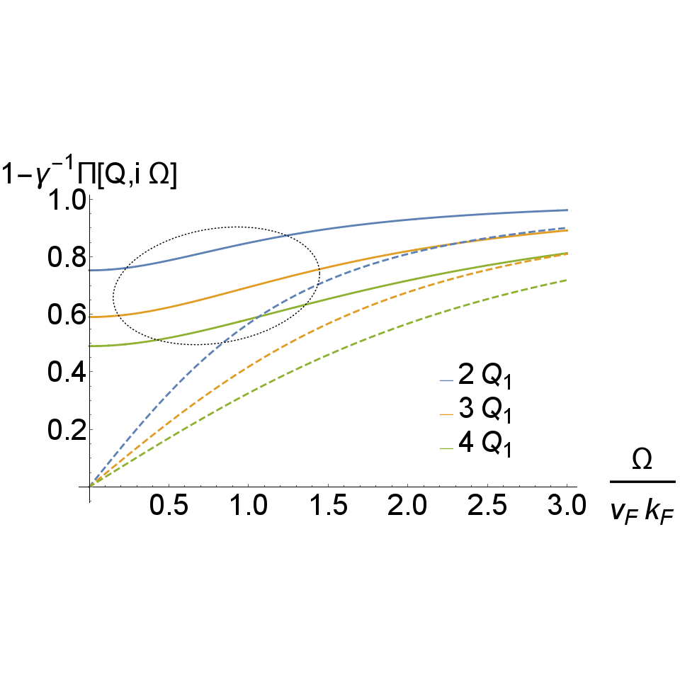
In this work we explore an additional, hitherto undiscussed aspect of the problem – a strong sensitivity of an itinerant QC system to finite-size effects. To separate this from the effects associated with the non-conservation of the nematic order parameter, we approximate the nematic form-factor by a constant, i.e., equate nematic fluctuations with fermionic density fluctuations. We show that in a finite system of size $L$, the polarization bubble, whose dynamical part yields the Landau damping at $L\to\infty$, is

When $q_{1}/q$ is vanishingly small, $\Pi(\alpha,\beta)=\gamma(1-\alpha/\sqrt{1+\alpha^{2}})$, as for an infinite system. At at a non-zero $\beta$, the form of $\Pi(\alpha,\beta)$ is determined by a combination of two effects: (i) $\Pi(0,\beta)$ decreases with increasing $\beta$ ($\Pi(\alpha,\beta)$ vanishes at $\beta=1$, see below), and (ii) $\Pi(\alpha,\beta)$ vanishes at $\alpha\to\infty$ for any $\beta$. As a result, there appears an intermediate range of $\alpha<1$, where the variation of $\Pi(\alpha,\beta)$ vs $\alpha$ (i.e., vs $|\Omega_{m}|$) is roughly linear, but the slope decreases as $\beta$ increases and over a rather wide range of parameters appears almost independent of $q$ (see Fig. 1a). This mimics $z=2$ scaling as reported in [17] (Fig. 1b). We also found that the data from Ref. [17] can be reproduced in an alternative, semi-phenomenological approach, by invoking the fact that in a finite system the polarization bubble vanishes not at $q=0$, but at at $q=q_{1}$, i.e. at $\beta=1$. Near $\beta=1$, $\Pi(\alpha,\beta)\propto(1-\beta)^{3/2}$ (see below). Assuming phenomenologically that this is the main finite-size effect, we approximate the frequency dependence of the polarization bubble as

This simple form reproduces the data from [17] to surprisingly good accuracy (see Fig. 1c).

The fermionic self-energy also has strong finite-size dependence. We found (for $\omega_{m}>0$)

where $\omega_{1}\sim v_{F}q_{1}$ up to logarithms (see Eq. (14) below). At $\omega\gg\omega_{1}$ this yields $\Sigma(\omega_{m})\propto\omega^{2/3}$, as in the infinite system. However, at smaller $\omega$, $\Sigma(\omega_{m})=a\omega_{m}+b\omega^{2}_{m}+...$ as in a FL. As a result, for probes at $\omega\geq\omega_{1}$, it looks as if the quasipartcle residue remains finite throughout the transition. We compared Eq. (3) with Ref. [17] and again found good agreement with QMC data (see Fig. 3).

Model calculations    We consider a 2D system of size $L\times L$. The system is composed of electrons hopping on a lattice and coupled to a scalar boson field. The free propagators of electrons and bosons are of the form,

where $v_{0}$ is the bosonic velocity, and $m=1/\xi$ goes to zero at the QCP. In a finite system the interaction can be written as

where $f_{\bm{\mathrm{k}}}$ is a form factor, the $\bm{\mathrm{q}},\bm{\mathrm{k}}$ sums are over the 1st bosonic and fermionic BZ’s respectively, and $g$ is a coupling constant. If we restrict our attention to states near the Fermi surface, we can rewrite the interaction as:

Here, $\epsilon_{k}=v_{F}(k-k_{F})$ measures the distance from the FS and $f(\theta)$ is the form-factor at the FS. We separate the effects due to order parameter non-conservation from finite-size effects, and focus on the latter, by setting $f(\theta)=1$. The function $\Phi$ is an indicator function due to finite size of a system. It accounts for the lack of $k-$states in an annulus of width $q_{1}$ around the FS (see Fig. 2 for visualization),

Let us recall the origin of the form $\Omega/v_{F}q$ for the polarization. It arises from the fact that for small enough $\Omega\ll v_{F}|\bm{\mathrm{q}}|$ there is always an electron-hole pair that can be resonantly excited, given by the condition $\Omega=\bm{\mathrm{v_{F}}}\cdot\bm{\mathrm{q}}=v_{F}q\cos\theta$, as long as the FS is closed. However, as Eq. (7) shows, in a finite system and for small enough $\bm{\mathrm{q}}$ it is not always possible to find such a pair. The reason for this is that in a finite system the border between filled and empty states is not a smooth curve but a series of “facades” (Fig. 2). At small enough momentum and frequency it is no longer possible to find a resonant pair that also conserves momentum. This gives a lower cutoff of $\Omega<v_{F}q\sim v_{F}q_{1}$ for the overdamped behavior of the bosonic excitations, which introduces the new scale $\beta=q_{1}/q$, leading to Eq. (1). For $\beta$ close to one, the suppression effect is proportional to $(1-\beta)^{3/2}$. To see this, note that as we move around the FS, the available phase space for particle-hole excitations is $\bm{\mathrm{v_{F}}}\cdot\bm{\mathrm{q}}-v_{F}q_{1}=v_{F}q(\cos\theta-\beta)$. Because of this restriction, the polarization bubble is proportional to

(we used $\theta_{\beta}\sim(1-\beta)^{1/2}$ for $1-\beta\ll 1$). This is the reasoning behind Eq. (2).

In addition to the damping term, the polarization bubble has a static piece, which renormalizes the bosonic mass and shifts the position of the QCP. This last term also gets modified in a finite system in such a way that the bosonic mass remains positive at a QCP of an infinite system, i.e., finite-size effects shift the system away from the critical point. This finite bosonic mass affects the self energy. In an infinite system $\Sigma(\bm{\mathrm{q}},\omega)\sim\omega^{2/3}$ displays a non-FL behavior at a QCP. In a finite-size system, the mass term protects the FL behavior at low frequencies, which is the content of Eq. (3).

We demonstrate this behavior by explicitly calculating the polarization bubble and the self energy for the approximate model of Eqs. (4)-(8). We assume a parabolic dispersion and calculate the one-loop diagrams. To calculate the one-loop polarization bubble at $T\to 0$ we take into account only those $k-$ states that are on opposite sides of the boundary of the Fermi surface. In this case the indicator function can be recast as

The polarization is then given by:

where $m_{0}$ is the bare fermionic mass. The limits of the integration are precisely those defined by the finite size effect of Eq. (10). Evaluating the integrals we find

where $\gamma=m_{0}g^{2}\chi_{0}/2\pi$. One can easily check that $\Pi(\alpha,\beta)$ vanishes at $\alpha\to\infty$ and at $\beta=1$. When $\beta\ll\alpha<1$, $\Pi(\alpha,\beta)\approx\gamma\left(1-\beta\log{2/\alpha}-\alpha\right)$ Near $\beta=1$, $\Pi(\alpha,\beta)\approx 1.2\gamma(1-\beta)^{3/2}/(1+\alpha^{2})$.

We next calculate the fermionic self-energy

where ${\tilde{\chi}}^{-1}=\chi^{-1}+\Pi$. We used the form of $\Pi$ at $\beta<\alpha\ll 1$ and absorbed the constant term in $\Pi$ into $m^{2}$. One can verify that the integral is dominated by $|\Omega_{m}|\sim\omega_{m},\hat{\bm{\mathrm{k}}}_{F}\cdot\bm{\mathrm{q}}\sim\omega_{m},\hat{\bm{\mathrm{k}}}_{F}\times\bm{\mathrm{q}}\sim\mbox{max}(|\Omega_{m}|,q_{1}\log 2/\alpha)^{1/3}$. Thus, in the range $\Omega_{m}<v_{F}q_{1}\log{\gamma^{1/2}/q_{1}}$ we can expand in the dynamic part of the susceptibility, which makes $\Sigma$ an analytic function of frequency. An evaluation of Eq. (13) at $m=0$ yields

where

Eq. (14) is the explicit version of Eq. (3). We plot $\Sigma(\omega_{m})$ along with QC and FL asymptotics ($\omega^{2/3}$ and $\omega$, respectively) in Fig. 3a. We see that in a finite-size system $\Sigma(\omega_{m})$ preserves a FL form up to large $\omega_{m}/v_{F}q_{1}$.

An additional popular probe in QMC is the Green’s function on the Fermi surface along the imaginary time axis [25],

In a FL, $G(\tau=T/2)=Z_{qp}/2$. For $\Sigma\sim\omega_{n}^{2/3}$ $G(\tau=T/2)=T^{1/3}$, indicating that the quasiparticle residue vanishes at $T=0$ (the actual power is $T^{1/2}$ due to special form of the self-energy at the first Matsubara frequency [26]). Because the sum is dominated by the terms with $n=O(1)$, the finite size behavior of $\Sigma$ is important. Plugging parameters extracted from the data of Ref. [17] into Eq. (14) and substituting into Eq. (16), we obtain $Z_{qp}$, which decreases as a function of $T$, but still approaches a finite value at $T\to 0$ (see Fig. 3b ). In this limit, our calculation yields $Z_{qp}=0.76$. Ref. [17] found a very similar $Z_{qp}=0.75-0.85$ in the low temperature regime ¹¹ 1 In order to compare our analytic expressions in Eqs. (4), (12), (14) with the QMC data, we used the average value of the Fermi vector and velocity $k_{F},v_{F}$ for a cubic lattice. We extracted the value of $\gamma$ by comparing the values of $\Pi(0,0)$ at $g=0$ and finite $g$. We extracted $c^{2}$ by fitting the data for $q=0$ to a quadratic form. The value of $\chi_{0}$ was taken from Ref. [17]..

Discussion.    We showed that finite size effects modify the low energy properties of the particle-hole polarization bubble and the fermionic self energy near a $q=0$ QCP. We found three effects: i) the slope of the frequency dependence of $\Pi(q,\Omega_{m})$ changes from its universal $1/q$ form to almost $q-$independent, ii) the bosonic mass gets a $q$ dependent correction; iii) the non-analyticity of the electronic self energy is cut off below a certain frequency. In a real finite-size system the strength of (i) and (ii) is actually a bit smaller than in our model, where the polarization appears to vanish at $q=q_{1}$ for all $\Omega_{m}$. In practice, there will always be a residual polarisation coming from a) broadening due to finite self energy, and b) the irregularity of the separation between filled/empty states due to a discrete structure of the FS in a finite system. Both these features can be seen just by studying the left panel of Fig. 2. A translational symmetry breaking inherent in any finite system also induces broadening. Nevertheless our results do capture the main features observed in QMC studies.

Our results can also be applied to magnetic conducting nanoparticles near a near a ferromagnetic/paramagnetic QCP. Magnetic nanoparticles have attracted attention in recent years due to biomedical and other applications. One implication is that the finite-size correction to the bosonic mass will introduce strong wavelength-dependent hysteresis in the region where $q(T-T_{c})\sim T_{c}/L$. Another is that for $|T-T_{c}|\leq T_{c}a/L$ the magnetic susceptibility saturates and the resistance obeys its Fermi liquid $T^{2}$ behavior. In a recent work [28], magnetic nanoparticles of composition Pd_1-xNi_x were tuned across the transition, as evidenced by their magnetic response. However, the resistance remained Fermi-liquid like. In a follow-up analysis [29] of Ni_1-xV_x, a decrease in the slope of $\chi(T)$ was observed, at $T\sim 5-10K$, even at the QCP ($T_{c}\sim 0$). In these systems, $a\simeq 3.5\mathring{A}$ and $L\simeq 20-40\mbox{nm}$. Combining this with bulk nickel’s Curie temperature $T_{c}\sim 600K$ (to be distinguished from the nanoparticle $T_{c}\sim 0$ at the QCP) we find a saturation temperature of $|T-T_{c}|=T_{c}a/L=5.5-11K$, in remarkable agreement with experimental results. We leave further analysis of such systems to future work.