Locality and Availability of Array Codes Constructed from Subspaces

Natalia Silberstein Tuvi Etzion Moshe Schwartz ^†^†thanks: The material in this paper was presented in part at the IEEE International Symposium on Information Theory (ISIT 2017), Aachen, Germany, June 2017.^†^†thanks: Natalia Silberstein was with the Department of Electrical and Computer Engineering, Ben-Gurion University of the Negev, Beer Sheva 8410501, Israel, and is now with Yahoo! Research, Haifa 31905, Israel, (e-mail: natalys@cs.technion.ac.il).^†^†thanks: Tuvi Etzion is with the Department of Computer Science, Technion – Israel Institute of Technology, Haifa 3200003, Israel, (e-mail: etzion@cs.technion.ac.il).^†^†thanks: Moshe Schwartz is with the Department of Electrical and Computer Engineering, Ben-Gurion University of the Negev, Beer Sheva 8410501, Israel (e-mail: schwartz@ee.bgu.ac.il).^†^†thanks: This work was supported in part by the NSF-BSF grant no.˜2016692, and by the Israeli Science Foundation (ISF), Jerusalem, Israel, under Grant no.˜130/14.

Abstract

We study array codes which are based on subspaces of a linear space over a finite field, using spreads, $q$ -Steiner systems, and subspace transversal designs. We present several constructions of such codes which are $q$ -analogs of some known block codes such as the Hamming and simplex codes. We examine the locality and availability of the constructed codes. In particular we distinguish between two types of locality and availability – node vs. symbol, locality and availability. The resulting codes have distinct symbol/node locality/availability, allowing a more efficient repair process for a single symbol, compared with the repair process for the whole node.

Index Terms:

Locally repairable codes, distributed storage, availability,

q

-analog

I Introduction

Designing efficient mechanisms to store, maintain, and efficiently access large volumes of data is a highly relevant problem. Indeed, ever-increasing amounts of information are being generated and processed in the data centers of Amazon, Facebook, Google, Dropbox, and many others. The demand for ever-increasing amounts of cloud storage is supplied through the use of Distributed Storage Systems (DSS), where data is stored on a network of nodes (hard drives and solid-state drives).

In the DSS paradigm, it is essential to store data redundantly, in order to tolerate inevitable node failures [2, 19, 41]. Currently, the resilience against node failures is typically the result of replication, where several copies of each data object are stored on different storage nodes. However, replication is highly inefficient in terms of storage capacity. Recently, erasure-correcting codes have been used in DSS to reduce the large storage overhead of replicated systems [8, 10, 24].

Apart from storage space, other metrics should be considered when designing an actual DSS. However, in contrast with storage space, these metrics are adversely affected by the straightforward use of simple erasure-correcting codes. One such metric is the repair bandwidth: the amount of data that needs to be transferred when a node has failed, and is thus replaced. This metric is highly relevant as a prohibitively large fraction of the network bandwidth in a DSS may be consumed by such repair operations. Let us term all the information stored by a DSS as the file. Traditional erasure-correcting codes, and in particular maximum distance separable (MDS) codes, usually require that all the file be downloaded in order to regenerate a failed node. Recently, Dimakis et al. [9] established a trade-off between the repair bandwidth and the storage capacity of a node, and introduced a new family of erasure-correcting codes, called regenerating codes, which attain this trade-off. In particular, they proved that if a large number of storage nodes can be contacted during the repair of a failed node, and only a fraction of their stored data is downloaded, then the repair bandwidth can be minimized.

Local repair of a DSS is an additional property which is highly sought. The corresponding performance metric is termed the locality of the coding scheme: the number of nodes that must participate in a repair process when a particular node fails. Local repair is of significant interest when a cost is associated with contacting each node in the system. This is indeed the case in real world scenarios, for example as the result of network constraints. Codes which enable local repairs of failed system nodes are called locally repairable codes (LRCs). These codes were introduced by Gopalan et al. in [20]. LRCs which also minimize the repair bandwidth, called codes with local regeneration, were considered in [28, 29, 37].

Regenerating codes and LRCs are attractive primarily for the storage of cold data – archival data that is rarely accessed. On the other hand, they do not address the challenges posed by the storage of frequently accessed hot data. For example, hot-data storage must enable efficient reads of the same data segments by several users in parallel. This property is referred to as availability. Codes which provide both locality and availability were first proposed in [39].

Recently, codes with locality and availability have found another application in the well known area of private information retrieval [7]. Shah, Rashmi, and Ramchandran [45] were the first to consider storage overhead for this important concept. In an important development, Fazeli, Vardy, and Yaakobi [15, 16] demonstrated how codes with good availability can be used to save storage and to obtain low storage overhead. Their new ideas have motivated a series of papers with related results, e.g., [3, 4, 17, 31, 35, 50, 51, 56]. Other codes which were studied in the context of private information retrieval are batch codes [26, 1]. These codes also have applications as distributed storage system codes [40].

Regenerating codes are described in terms of stored information in nodes (servers). In other words, regenerating codes are usually array codes [49]. Reconstructing the files and repairing failed nodes are the main tasks of regenerating codes. LRCs and codes with availability are usually described as block codes, and access and/or repair is described in terms of symbols.

In this work we combine the two approaches and discuss two types of locality (respectively, availability): node locality (availability), which resembles the first approach, and symbol locality (availability), which resembles the second approach. To our knowledge, such a combined approach was not considered in the literature before.

Our solution approach will be based on array codes, constructed via subspaces of a finite vector space. A subspace approach for DSS codes was considered for the first time in [22] and later in [36]. Our approach is slightly different from the approach in these two papers. We shall employ spreads, $q$ -Steiner systems, and subspace transversal designs in our constructions. We will also analyze the node and symbol, locality and availability, of the resulting codes. This subspace approach for locality and availability is also novel.

I-A Our Contribution

In this paper we present several constructions of array codes. The parameters of these codes are summarized in Table I. Note, that $r_{\mathrm{s}}$ and $r_{\mathrm{n}}$ denote symbol locality and node locality, respectively, and $t_{\mathrm{s}}$ and $t_{\mathrm{n}}$ denote the symbol availability and node availability, respectively (for formal definitions see Definitions 1-3 in the following section).

•

Construction A is based on all the $b$ -dimensional subspaces of ${{\mathbb{F}}}_{\!q}^{M}$ . When $b=1$ , it yields the classic simplex code, and hence it can be considered as its generalization and $q$ -analog.
•

Construction B is based on a $b$ -spread of ${{\mathbb{F}}}_{\!q}^{M}$ , which are very important and well studied in projective geometry (see the definition of a $b$ -spread in Section III-B). This construction also yields the simplex code when $b=1$ , and when $M=2b$ , it yields an MDS array code. Moreover, its dual code is a perfect array code (see Lemma 7).
•

Construction A and Construction B are based on the two extreme cases of the $q$ -analog of combinatorial designs. More generally, we provide Construction C, which generalizes the previous two constructions. It uses the $q$ -analog of block designs, namely, $q$ -Steiner systems. However, there is only one set of parameters (apart from the parameters of Constructions A and B) where they are known to exist. Nonetheless, it is conjectured that infinite families of such designs exist (see Section III-B).
•
Construction D is based on a subspace transversal design. These designs have similar properties to the the ones of $q$ -Steiner systems, but unlike them, subspace transversal designs are known to exist for many parameters (see the definition of a subspace transversal design in Section III-B). In particular, we consider two types of constructions from subspace transversal designs, namely
1. 1.
  
  based on a single parallel class of a subspace transversal design;
2. 2.
  
  based on all the subspaces in a subspace transversal design.
When $M=2b$ , the first construction produces an MDS array code. In addition, the dual code of the code obtained from this construction is an asymptotically perfect array code.

TABLE I: Parameters of the constructed codes.

Reference	$\mathbf{[b\times n,M,d]}$	Symbol locality	Node locality
Construction A	$[b\times\genfrac{[}{]}{0.0pt}{}{M}{b},M,q^{M-b}\genfrac{[}{]}{0.0pt}{}{M-1}{b -1}]$	$r_{\mathrm{s}}=\begin{cases}1&1<b<M,\\ 2&b=1.\end{cases}$	$r_{\mathrm{n}}=2$
Construction B	$[b\times\frac{q^{M}-1}{q^{b}-1},M,q^{M-b}]$	$r_{\mathrm{s}}=2$	$2\leqslant r_{\mathrm{n}}\leqslant b+1$
Construction D.1	$[b\times q^{M-b},M,q^{M-b}-q^{M-2b}]$	$r_{\mathrm{s}}=2$	$r_{\mathrm{n}}=\begin{cases}3&q=2,\\ 2&q>2.\end{cases}$
Construction D.2	$[b\times q^{(M-b)t},M,q^{(M-b)(t-1)}(q^{M-b}-q^{M-2b})]$	$r_{\mathrm{s}}=1$	$r_{\mathrm{n}}\geqslant 2$

In addition to the node and symbol locality of the constructed codes summarized in Table I, we have node and symbol availability for some of the codes. The code from Construction A has symbol availability

t_{\mathrm{s}}=\begin{cases}\genfrac{[}{]}{0.0pt}{}{M-1}{b-1}-1&1<b<M,\\ \frac{q^{M-1}-1}{2}&b=1.\end{cases}

and node availability

t_{\mathrm{n}}=\begin{cases}\frac{1}{2}\left(\genfrac{[}{]}{0.0pt}{}{M}{2}-1\right)&2=b<M,\text{even }q\\ \geqslant\frac{1}{2}\left(\genfrac{[}{]}{0.0pt}{}{M}{2}-1-q(q^{2}+q-1)\genfrac{[}{]}{0.0pt}{}{M-2}{2}\right)&2=b<M,\text{odd }q.\end{cases}.

The symbol availability of the code from Construction D (the one based on all the subspaces in a subspace transversal design) is $t_{\mathrm{s}}=q^{(M-b)(t-1)}-1$ .

I-B Related Constructions

Codes with locality $r$ and availability $t$ allow us to recover any code symbol by using $t$ disjoint sets of cardinality $r$ (usually for $r$ relatively small). This line of research has been extremely active in the last few years as a consequence of its practical importance. The results of some known code constructions with locality and availability and their generalizations, mainly related to the constructions presented in this paper, are summarized below. We note that our combined approach, that distinguishes between node and symbol locality and availability, was not considered before. Many known constructions in the literature are not array codes, therefore precluding the distinction between nodes and symbols. Thus, actual comparison with previous works is mostly impossible, except for one simple case mentioned below.

•

Codes with locality and availability. Constructions of codes with locality and availability were proposed in [25, 39, 34, 48, 53]. Specifically, the construction presented in [34] is based on partial geometries. Resolvable combinatorial designs, and modified pyramid codes were used in [39]. The approach in [48] is based on orthogonal partitions and on product codes. One-step majority-logic decodable codes and product codes are used in [25].
•

Codes with locality and availability over small fields. Codes over small alphabets (and in particular, binary codes) are of particular interest due to their simple implementation. The locality properties of the family of binary simplex codes were proved in [6]. Modifications of simplex codes based on anticodes technique yield optimal codes with good locality and availability properties, as shown in [47]. Binary cyclic LRCs were considered in [21, 54]. Binary codes for any given locality $r$ and availability $t$ are provided in [53].
•

Codes with local regeneration. Codes that combine the properties of LRCs with regenerating codes, by allowing to minimize the repair bandwidth locally, were presented in [28, 29, 37]. Most of these codes (i.e., [29, 37]) are based on the properties of linearlized polynomials. To the best of our knowledge, these are the only previously known array codes that have locality properties. However, the locality for these codes is defined only for nodes, and the symbol locality appears to be hard to extract from the construction.
•

Other extensions and generalizations of LRCs. Codes that enable cooperative local recovery from multiple erasures were presented in [38]. In other words, these codes allow to recover any small set of codeword symbols from a small number of other symbols. Codes where symbols have different localities were considered in [55, 27]. Codes with hierarchical locality, which enable local recovery from multiple erasures were presented in [42]. The PIR array codes considered in [3, 4] have optimal symbol availability, with symbol locality 2, for large number of nodes, but their node locality and availability were not considered and again, appear to be hard to extract.
•

Fractional repetition codes. Construction of such codes, e.g., in [11, 30, 57, 46], provide arrays of repeating symbols. These were not intended originally for node and symbol locality and availability. However, their relatively simple structure allows us to find their parameters or bound them. In the notation of [46], an $(n,\alpha,\rho)$ -FR code (Fractional Repetition code) is composed of $\alpha\times n$ arrays with $\theta\triangleq n\alpha/\rho$ information symbols, each appearing in $\rho$ distinct columns. Thus, trivially, the symbol locality is $r_{\mathrm{s}}=1$ , the symbol availability is $t_{\mathrm{s}}=\rho-1$ . For nodes we have the trivial upper bounds of $r_{\mathrm{n}}\leqslant\alpha$ and $t_{\mathrm{n}}\leqslant\rho-1$ . In [46] we find three constructions of FR codes: $[\alpha\times n,\alpha n/2,2]$ codes, $[\alpha\times\rho\alpha,\alpha^{2},\rho]$ codes for $\rho\geqslant 3$ , and $[(t+1)\times(s+1)(st+1),(t+1)(st+1),s+1]$ codes for $t\geqslant s$ (with further restrictions described in detail in [46]). However, the main disadvantage of these codes, compared with the codes we construct (see Table I) is their low minimum distance.

I-C Paper Organization

The rest of this paper is organized as follows. Preliminaries are given in Section II. Our subspace approach, constructions of codes, and analysis of their locality and availability, are presented in Section III. We conclude in Section IV with a short discussion and some open problems.

II Preliminaries

Let $\mathbb{F}_{q}$ denote the finite field of size $q$ . For a natural number $m\in{\mathbb{N}}$ , we use the notation $[m]\triangleq\left\{1,2,\dots,m\right\}$ . We use lower-case letters to denote scalars. Overlined letters denote vectors, which by default are assumed to be column vectors. Matrices are denoted by upper-case letters. However, the codewords of array codes, which are arrays (matrices), will be denoted by bold lower-case letters. Thus, typically, we shall have a generator matrix $G$ , whose $j$ th column is $\overline{g}_{j}$ , and whose $(i,j)$ th entry is $g_{i,j}$ . An array code will usually be denoted by $C$ , whose typical codeword will be denoted by $\mathbf{c}$ . We use $0$ to denote the scalar zero, $\overline{0}$ for the all-zero column vector, and $\mathbf{0}$ for the all-zero matrix. Also, given a (possibly empty) set of vectors, $v_{1},\dots,v_{m}\in\mathbb{F}_{q}^{n}$ , their span is denoted by $\left\langle{v_{1},\dots,v_{m}}\right\rangle$ .

Our main object of study is a linear array code, formally defined as follows.

Definition 1

. A $[b\times n,M,d]$ array code over $\mathbb{F}_{q}$ , denoted $C$ , is a linear subspace of $b\times n$ matrices over $\mathbb{F}_{q}$ . Matrices $\mathbf{c}\in C$ are referred to as codewords. The elements of a codeword are denoted by $c_{i,j}$ , $i\in[b]$ , $j\in[n]$ , and are referred to as symbols. Columns of codewords are denoted by $\overline{c}_{j}$ , $j\in[n]$ . We denote by $M\triangleq\dim(C)$ the dimension of the code as a linear space over $\mathbb{F}_{q}$ . The weight of an array is defined as the number of non-zero columns, i.e., for $\mathbf{c}\in C$ ,

\wt(\mathbf{c})\triangleq\left|\left\{\overline{c}_{j}~:~\overline{c}_{j}\neq\overline{0},j\in[n]\right\}\right|.

Finally, the minimum distance of the code, denoted $d$ , is the defined as the minimal weight of a non-zero codeword,

d\triangleq\min_{\begin{subarray}{c}\mathbf{c}\in C\\ \mathbf{c}\neq\mathbf{0}\end{subarray}}\wt(\mathbf{c}).

We make two observations to avoid confusion with other notions of error-correcting codes. The first observation is that by reading the symbols of codewords, column by column, and within each column, from first to last entry, we may flatten the $b\times n$ codewords to vectors of length $bn$ . This results in a code over $\mathbb{F}_{q}$ of length $bn$ , dimension $M$ , but more often than not, a different minimum distance, since the above definition considers non-zero columns and not non-zero symbols. Assume $G$ is an $M\times bn$ generator matrix for the flattened code. By abuse of notation, we shall also call $G$ the generator matrix for the original array code $C$ . Note that in $G$ , columns $(j-1)b+1,\dots,jb$ , correspond to the symbols appearing in the $j$ th codeword column in $C$ . We shall call these $b$ columns in $G$ by the $j$ th thick column of $G$ , similarly to [28]. Thus, $G$ is a matrix comprised of $n$ thick columns, corresponding to the $n$ columns of codewords in $C$ .

Example 1

. Over $\mathbb{F}_{2}$ , let $C$ be a $[2\times 5,5,3]$ array code, and let

\mathbf{c}=\begin{pmatrix}0&0&0&0&1\\ 0&1&1&0&0\end{pmatrix}

be a codeword of $C$ with weight 3. The corresponding flattened codeword is $(0001010010)$ , which is exactly the last row of the following generator matrix $G$ for $C$ ,

G=\left(\begin{array}[]{c|c|c|c|c}10&00&01&01&00\\ 00&10&00&01&01\\ 01&00&10&00&01\\ 01&01&00&10&00\\ 00&01&01&00&10\end{array}\right),

which has 5 thick columns (separated by vertical lines). $\Box$

The second observation is that we may use the well known isomorphism $\mathbb{F}_{q}^{b}\cong\mathbb{F}_{q^{b}}$ , and consider each column of a codeword as a single element from $\mathbb{F}_{q^{b}}$ . We get an $\mathbb{F}_{q}$ -linear code over $\mathbb{F}_{q^{b}}$ (sometimes called a vector-linear code), of length $n$ , minimum distance $d$ , but with a dimension (taken as usual over $\mathbb{F}_{q^{b}}$ ) not necessarily $M$ .

In a typical distributed-storage setup, we would like to store a file containing $M$ sectors. We choose $\mathbb{F}_{q}$ such that it is large enough to contain all possible sectors as symbols. The file is encoded into an array $\mathbf{c}\in C$ from a $[b\times n,M,d]$ array code. Each codeword column of $\mathbf{c}$ is stored in a different node. The minimum distance $d$ of the code ensures that any failure of at most $d-1$ nodes may be corrected. Figure 1 illustrates this idea using the code from Example 1.

Refer to caption — Figure 1: Distributed storage system based on the binary $[2\times 5,5,3]$ array code from Example 1.

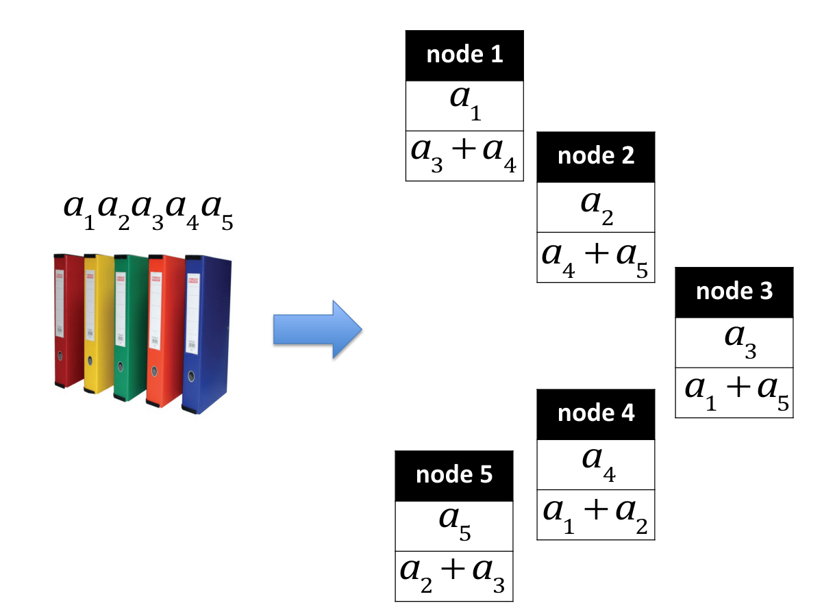
Two important properties of codes for distributed storage are locality and availability. An important feature of this paper is the distinction between symbol locality and node locality (respectively, availability). Note that this approach is different from the standard one, where only node locality and availability are considered. The motivation to explore codes with different types of locality and availability is the problem of latent sector errors (LSEs), where individual sectors (symbols) on a drive (node) become unavailable [43]. As can be observed in the sequel, symbol locality can be smaller when compared to the node locality. Thus, a more efficient recovery of a single symbol is possible, compared with the recovery of an entire node, since fewer nodes need to be contacted. Similarly, symbol availability can be larger when compared to the node availability, which also enhances the recovery process of a single symbol compared with an entire node.

Definition 2

. Let $C$ be a $[b\times n,M,d]$ array code. We say a codeword column $j\in[n]$ has node locality $r_{\mathrm{n}}$ , if its content may be obtained via linear combinations of the contents of the recovery-set columns. More precisely, there exists a recovery set $S=\left\{j_{1},\dots,j_{r_{\mathrm{n}}}\right\}\subseteq[n]\setminus\left\{j\right\}$ of $r_{\mathrm{n}}$ other codeword columns, and scalars $a_{\ell,m}^{(i)}\in\mathbb{F}_{q}$ , $i,\ell\in[b]$ , $m\in[r_{\mathrm{n}}]$ , such that for all $i\in[b]$ ,

c_{i,j}=\sum_{m=1}^{r_{\mathrm{n}}}\sum_{\ell=1}^{b}a_{\ell,m}^{(i)}c_{\ell,j_{m}}

(1)

simultaneously for all codewords $\mathbf{c}\in C$ . If all codeword columns have this property, we say the code has node locality of $r_{\mathrm{n}}$ .

Similarly, we say the code has symbol locality $r_{\mathrm{s}}$ , if for every coordinate, $i\in[b]$ and $j\in[n]$ , there exists a recovery set $S=\left\{j_{1},\dots,j_{r_{\mathrm{s}}}\right\}\subseteq[n]\setminus\left\{j\right\}$ of $r_{\mathrm{s}}$ other codeword columns, and scalars $a_{\ell,m}\in\mathbb{F}_{q}$ , $\ell\in[b]$ , $m\in[r_{\mathrm{s}}]$ , such that for every codeword $\mathbf{c}\in C$ ,

c_{i,j}=\sum_{m=1}^{r_{\mathrm{s}}}\sum_{\ell=1}^{b}a_{\ell,m}c_{\ell,j_{m}}.

(2)

Thus, each code symbol may be recovered from the code symbols in $r_{\mathrm{s}}$ other codeword columns.

Note that the coefficients in (2) are not necessarily the same as those in (1). Additionally, it is obvious that $r_{\mathrm{s}}\leqslant r_{\mathrm{n}}$ .

Once locality is defined, we can also define availability.

Definition 3

. The node availability, denoted $t_{\mathrm{n}}$ , (respectively, the symbol availability, denoted $t_{\mathrm{s}}$ ) is the number of pairwise-disjoint recovery sets (as in the definition of locality) that exist for any codeword column (respectively, symbol). Note that each recovery set should be of size at most $r_{\mathrm{n}}$ (respectively, $r_{\mathrm{s}}$ ).

Example 2

. One can verify that the code from Example 1 has symbol locality $r_{\mathrm{s}}=2$ , but node locality $r_{\mathrm{n}}=3$ . Additionally, it has symbol availability $t_{\mathrm{s}}=2$ , but node availability $t_{\mathrm{n}}=1$ . $\Box$

We also recall some useful facts regarding Gaussian coefficients. Let $V$ be a vector space of dimension $n$ over $\mathbb{F}_{q}$ . For any integer $0\leqslant k\leqslant n$ , we denote by $\genfrac{[}{]}{0.0pt}{}{V}{k}$ the set of all $k$ -dimensional subspaces ( $k$ -subspaces, in short) of $V$ . The Gaussian coefficient is defined for $n$ , $k$ , and $q$ as

\displaystyle\genfrac{[}{]}{0.0pt}{}{n}{k}_{q}

\displaystyle\triangleq\frac{(q^{n}-1)(q^{n-1}-1)\dots(q^{n-k+1}-1)}{(q^{k}-1)(q^{k-1}-1)\dots(q-1)}.

Whenever the size of the field, $q$ , is clear from the context, we shall remove the subscript $q$ .

It is well known that the number of $k$ -subspaces of an $n$ -dimensional space over $\mathbb{F}_{q}$ is given by $\genfrac{[}{]}{0.0pt}{}{n}{k}$ . In a more general form, the number of $k^{\prime}$ -subspaces of $V$ which intersect a given $k$ -subspace of $V$ in an $i$ -subspace is given by

q^{(k^{\prime}-i)(k-i)}\genfrac{[}{]}{0.0pt}{}{n-k}{k'-i}\genfrac{[}{]}{0.0pt}{}{k}{i}.

(3)

Additionally, the Gaussian coefficients satisfy the following recursions,

	$\displaystyle\genfrac{[}{]}{0.0pt}{}{n}{k}$	$\displaystyle=\genfrac{[}{]}{0.0pt}{}{n-1}{k}+q^{n-k}\genfrac{[}{]}{0.0pt}{}{n-1}{k-1}$
		$\displaystyle=q^{k}\genfrac{[}{]}{0.0pt}{}{n-1}{k}+\genfrac{[}{]}{0.0pt}{}{n-1}{k-1}.$		(4)

For more on Gaussian coefficients, the reader is referred to [52, Chapter 24].

III A Subspace Approach to LRCs

Let $C$ be a $[b\times n,M,d]$ array code over $\mathbb{F}_{q}$ . Throughout this section we further assume that $b\leqslant M$ . We now describe an approach to viewing such array codes which will lead to the main results of this section.

Denote $V\triangleq\mathbb{F}_{q}^{M}$ the $M$ -dimensional vector space over $\mathbb{F}_{q}$ . Let $G$ be a generator matrix for the (flattened) array code $C$ . For each $j\in[n]$ , we define $V_{j}$ , such that $V_{j}\in\bigcup_{k=0}^{b}\genfrac{[}{]}{0.0pt}{}{V}{k}$ , to be the column space of the $j$ th thick column of $G$ , i.e.,

V_{j}\triangleq\left\langle{\overline{g}_{(j-1)b+1,},\overline{g}_{(j-1)b+2},\dots,\overline{g}_{jb}}\right\rangle.

We say $V_{j}$ is associated with the $j$ th thick column of $G$ , or equivalently, associated with the $j$ th column of the codewords of $C$ .

Example 3

. The $2$ -dimensional vector space associated with the second thick column of the code from Example 1 is $V_{2}=\left\langle{(01000)^{T},(00011)^{T}}\right\rangle$ . $\Box$

The following equivalence is fundamental to the constructions and analysis of this section.

Lemma 1

. Let $C$ be a $[b\times n,M,d]$ array code over $\mathbb{F}_{q}$ , and let $V_{j}$ , $j\in[n]$ , be the subspaces associated with the codeword columns. Then $S=\left\{j_{1},\dots,j_{m}\right\}\subseteq[n]\setminus\left\{j\right\}$ is a recovery set for codeword column $j\in[n]$ , if and only if

V_{j}\subseteq V_{j_{1}}+V_{j_{2}}+\dots+V_{j_{m}}.

Similarly, $S$ is a recovery set for symbol $(i,j)$ , $i\in[b]$ , if

\overline{g}_{(j-1)b+i}\in V_{j_{1}}+V_{j_{2}}+\dots+V_{j_{m}},

where $\overline{g}_{(j-1)b+i}$ is the $i$ th column in the $j$ th thick column of a generating matrix $G$ for $C$ .

Proof:

This is a simple restatement of (1) and (2).

With this equivalence, we may obtain the node/symbol locality/availability using subspace properties of the thick columns of a generating matrix. Another definition of interest is the following.

Definition 4

. Let $C$ be a $[b\times n,M,d]$ array code over $\mathbb{F}_{q}$ , and let $V_{j}$ be the subspace associated with the $j$ th thick column. If $\dim(V_{j})=b$ for all $j\in[n]$ we call $C$ full column rank.

III-A Generalized Simplex Codes via Subspaces

We start with a construction of array codes which may be considered as a generalization and a $q$ -analog of the classical simplex code, the dual of the Hamming code (see [32, p. 30]).

Construction A

. Fix a finite field $\mathbb{F}_{q}$ , positive integers ${1\leqslant b\leqslant M}$ , and $V=\mathbb{F}_{q}^{M}$ . Construct a $b\times\genfrac{[}{]}{0.0pt}{}{M}{b}$ array code whose set of columns are associated with the subspaces $\genfrac{[}{]}{0.0pt}{}{V}{b}$ , each appearing exactly once. To make the dependence on the code parameters explicit, we denote this code by $C_{b}^{M}$ .

Note that when we choose $b=1$ in Construction A we obtain the simplex code. This fact will be used in the proof of Theorem 1 below.

We make a note here, which is also relevant for the constructions to follow. Once we fix the set of subspaces associated with the codeword columns, the code is constructed in the following way: for each $j\in[n]$ , and associated subspace $V_{j}$ , we arbitrarily choose a set of $b$ vectors from $\mathbb{F}_{q}^{M}$ that form a basis for $V_{j}$ . These $b$ vectors are placed (in some arbitrary order) as the columns comprising the $j$ th thick column of a generator matrix $G$ . The resulting matrix $G$ generates the constructed code¹¹ 1 Permuting the thick columns in the construction results in equivalent codes. If a canonical representation is required, we may choose the basis of each thick column to be in reduced row echelon form..

Lemma 2

. Fix a finite field $\mathbb{F}_{q}$ , positive integers $b<M$ , and $V=\mathbb{F}_{q}^{M-1}$ . For any $V^{\prime}\in\genfrac{[}{]}{0.0pt}{}{V}{b-1}$ , given as the column space of an $(M-1)\times(b-1)$ matrix $G^{\prime}$ , and for any non-zero vector $\overline{u}\in\mathbb{F}_{q}^{M-1}$ such that $\overline{u}^{T}G^{\prime}=\overline{0}^{T}$ , the following hold:

1.

If $\overline{x},\overline{y}\in\mathbb{F}_{q}^{M-1}$ are in the same coset of $V^{\prime}$ , then $\overline{u}^{T}\overline{x}=\overline{u}^{T}\overline{y}$ .
2.

The number of cosets of $V^{\prime}$ , all of whose vectors $\overline{x}$ satisfy $\overline{u}^{T}\overline{x}=a$ , for some fixed $a\in\mathbb{F}_{q}$ , is exactly $q^{M-b-1}$ .

Proof:

Denote the columns of $G^{\prime}$ as $\overline{g}^{\prime}_{1},\dots,\overline{g}^{\prime}_{b-1}$ . If $\overline{x}$ and $\overline{y}$ are in the same coset of $V^{\prime}$ , then there exist scalars $a_{1},\dots,a_{b-1}$ such that

\overline{x}=\overline{y}+\sum_{j=1}^{b-1}a_{j}\overline{g}^{\prime}_{j}.

Multiplying on the left by $\overline{u}^{T}$ , and recalling that $\overline{u}^{T}G^{\prime}=\overline{0}^{T}$ , we obtain the first claim.

The number of cosets of $V^{\prime}$ is exactly $q^{M-b}$ , each containing $q^{b-1}$ vectors. Since $\overline{u}\neq\overline{0}$ , the number of vectors $\overline{x}\in\mathbb{F}_{q}^{M-1}$ such that $\overline{u}^{T}\overline{x}=a$ is $q^{M-2}$ . Dividing this by the number of vectors per coset we obtain the second claim.

We are now ready for the first claim on the properties of the codes from Construction A.

Theorem 1

. The array code obtained from Construction A is a $[b\times\genfrac{[}{]}{0.0pt}{}{M}{b},M,d]$ array code, with

d=\genfrac{[}{]}{0.0pt}{}{M}{b}-\genfrac{[}{]}{0.0pt}{}{M-1}{b}=q^{M-b}\genfrac{[}{]}{0.0pt}{}{M-1}{b -1}.

Additionally, except for the all-zero array codeword, all other codewords have the same constant weight $d$ .

Proof:

Apart from the minimum distance of the code, all other parameters are trivial. We shall prove the minimum distance property by proving the constant-weight property of the non-zero codewords by induction on $M$ and $b$ (we refer to this induction as induction A). Additionally, we assert an auxiliary claim on the thick columns of the generator matrix, namely, that each thick column has rank $b$ . We will prove this claim by induction as well (we refer to this second induction as induction B).

For the basis of induction A we have the following cases. When considering $C_{M}^{M}$ , the codewords are $M\times 1$ arrays, and trivially, any non-zero codeword has weight

1=q^{M-M}\genfrac{[}{]}{0.0pt}{}{M-1}{M-1}.

Another base case is $C_{1}^{M}$ . In the resulting generator matrix, each thick column contains just a single column, and the matrix is nothing but a generator matrix for the well known simplex code. The codewords are $1\times(q^{M}-1)/(q-1)$ arrays. The weight of the non-zero codewords in the simplex code is known to be $q^{M-1}$ , and indeed we get a constant weight of

q^{M-1}=q^{M-1}\genfrac{[}{]}{0.0pt}{}{M-1}{0}.

We additionally note that in both cases, each thick column has rank $b$ , i.e., the basis for induction B holds.

Assume now the claim holds for $C_{b-1}^{M-1}$ and for $C_{b}^{M-1}$ , for both inductions, A and B. For the induction step we prove the claim also holds for $C_{b}^{M}$ . Let their respective generating matrices be $G_{b-1}^{M-1}$ and $G_{b}^{M-1}$ . Since we are not in any of the induction-base cases, we additionally have $1<b<M$ .

We construct a new matrix, $G$ by concatenating modified thick columns from $G_{b-1}^{M-1}$ and $G_{b}^{M-1}$ . We first take each thick column of $G_{b}^{M-1}$ , append a bottom row of all zeros, and place it as a thick column of $G$ . We call these columns thick columns of type I.

All the remaining thick columns of $G$ , which we call of type II, are formed by the thick columns of $G_{b-1}^{M-1}$ as follows. Consider such a single thick column, which is an $(M-1)\times(b-1)$ matrix on its own. Denote its column space by $V^{\prime}\subseteq\mathbb{F}_{q}^{M-1}$ , which by the hypothesis of induction B, has rank $b-1$ . Thus, there are $q^{M-b}$ cosets of $V^{\prime}$ in $\mathbb{F}_{q}^{M-1}$ . Let $\overline{v}^{\prime}_{1},\dots,\overline{v}^{\prime}_{q^{M-b}}$ be arbitrary coset representatives of the distinct cosets of $V^{\prime}$ . We create $q^{M-b}$ thick columns in $G$ from the given thick column of $G_{b-1}^{M-1}$ by placing it, each time with $\overline{v}^{\prime}_{i}$ as a $b$ th column, and with an appended bottom row of $0,\dots,0,1$ . In such thick columns of type II, the left $b-1$ coordinates are called the recursive part, whereas the last coordinate is called the coset part. The two types of thick columns of $G$ (depending on their source) are depicted in Figure 2.

\begin{array}[]{|c|}\hline\cr\\ \\ \text{(a)}\\ \\ \\ \hline\cr 0,0,\dots,0,0\\ \hline\cr\end{array}\qquad\qquad\begin{array}[]{|c|c|}\hline\cr&\\ &\\ \text{(b)}&\overline{v}^{\prime}_{i}\\ &\\ &\\ \hline\cr 0,\dots,0&1\\ \hline\cr\end{array}

Figure 2: The two types of thick columns in the constructed matrix

G

: a type I thick column, created by a thick column (a) from

G_{b}^{M-1}

, and a type II thick column, created by a thick column (b) from

G_{b-1}^{M-1}

and one of its column-space coset representatives.

Simple bookkeeping shows that we have $\genfrac{[}{]}{0.0pt}{}{M-1}{b}$ thick columns of type I, and $q^{M-b}\genfrac{[}{]}{0.0pt}{}{M-1}{b}$ thick columns of type II, for a total of

\genfrac{[}{]}{0.0pt}{}{M-1}{b}+q^{M-b}\genfrac{[}{]}{0.0pt}{}{M-1}{b-1}=\genfrac{[}{]}{0.0pt}{}{M}{b}

thick columns, where we used (4). They are easily seen to have distinct associated subspaces, each of dimension $b$ , accounting for all the $b$ -subspaces of $V=\mathbb{F}_{q}^{M}$ . Thus, $G$ is indeed a generator matrix for the code from Construction A, where each column has rank $b$ .

Now that we have proven a decomposition for the generator matrix $G$ , we can proceed with the proof of the constant weight of all non-zero codewords. It is easily seen that $G$ has full rank. We consider several cases, depending on the rows of $G$ participating in the linear combination creating the codeword at question.

In the simplest case, if a codeword of $C_{b}^{M}$ is formed by the last row of $G$ only, then its weight is $q^{M-b}\genfrac{[}{]}{0.0pt}{}{M-1}{b-1}$ , as the number of thick columns of type II.

For the second case, let us consider a codeword $\mathbf{c}\in C_{b}^{M}$ formed by a linear combination of some rows from the first $M-1$ rows of $G$ . By the hypothesis of induction A, the thick columns of type I contribute $\genfrac{[}{]}{0.0pt}{}{M-1}{b}-\genfrac{[}{]}{0.0pt}{}{M-2}{b}$ to the weight of $\mathbf{c}$ . Also by the hypothesis of induction A, the recursive parts of thick columns of type II contribute $q^{M-b}(\genfrac{[}{]}{0.0pt}{}{M-1}{b-1}-\genfrac{[}{]}{0.0pt}{}{M-2}{b-1})$ to the weight. Finally, even if for some thick column of type II the recursive part may produce a combination of all zeros, the coset part may be non-zero, thus contributing to the weight of $\mathbf{c}$ . More precisely, we have $\genfrac{[}{]}{0.0pt}{}{M-2}{b-1}$ recursive parts the linear combination zeros. Therefore, by Lemma 2, the coset part of exactly $\genfrac{[}{]}{0.0pt}{}{M-2}{b-1}(q-1)q^{M-b-1}$ becomes non-zero, and contributes to the weight of $\mathbf{c}$ . In total we get,

	$\displaystyle\wt(\mathbf{c})$	$\displaystyle=\genfrac{[}{]}{0.0pt}{}{M-1}{b}-\genfrac{[}{]}{0.0pt}{}{M-2}{b}$
		$\displaystyle\quad\ +q^{M-b}\left(\genfrac{[}{]}{0.0pt}{}{M-1}{b-1}-\genfrac{[}{]}{0.0pt}{}{M-2}{b-1}\right)$
		$\displaystyle\quad\ +\genfrac{[}{]}{0.0pt}{}{M-2}{b-1}(q-1)q^{M-b-1}$
		$\displaystyle=\genfrac{[}{]}{0.0pt}{}{M}{b}-\genfrac{[}{]}{0.0pt}{}{M-1}{b}.$

Finally, we consider a linear combination that, non-trivially, uses some rows from the set of $M-1$ first rows, as well as the last row. The $1$ ’s in the last row are located exactly at the coset part of thick columns of type II. Since by Lemma 2, the linear combination results in an equal number of appearances of each element of $\mathbb{F}_{q}$ in the coset parts, an addition of a multiple of the last row will not change that, and the weight of the codeword remains the same as in the previous case.

Lemma 3

. The array code obtained from Construction A, with parameters $b<M$ , has node locality of $r_{\mathrm{n}}=2$ , and symbol locality of

r_{\mathrm{s}}=\begin{cases}1&b>1,\\ 2&b=1.\end{cases}

Proof:

Let $C$ be a code generated by Construction A with a generator matrix $G$ . We first examine the case of $b>1$ . For symbol locality, given any column of $G$ , denoted $\overline{g}\in\mathbb{F}_{q}^{M}$ , by (3), there are exactly $\genfrac{[}{]}{0.0pt}{}{M-1}{b-1}$ $b$ -subspaces of $\mathbb{F}_{q}^{M}$ containing $\overline{g}$ , each corresponding to a thick column of $G$ . Since $b<M$ , we have $\genfrac{[}{]}{0.0pt}{}{M-1}{b-1}>1$ , and there exists a thick column different than the one containing the column $\overline{g}$ , whose column space contains $\overline{g}$ . Hence, $r_{\mathrm{s}}=1$ .

For node locality, given any subspace $V_{j}$ associated with the $j$ th thick column of $G$ , we can easily find two other subspaces $V_{j_{1}}$ and $V_{j_{2}}$ , $j\not\in\left\{j_{1},j_{2}\right\}$ , such that $V_{j}\subseteq V_{j_{1}}+V_{j_{2}}$ . For example: fix a basis for $V_{j}$ . Take the first basis element and complete it to a basis of some $b$ -subspace of $\mathbb{F}_{q}^{M}$ , denoted $V_{j_{1}}$ . Take the remaining $b-1$ basis elements of $V_{j}$ and complete them to a different $b$ -subspace, denoted $V_{j_{2}}$ . This can always be done when $1<b<M$ . Hence, $r_{\mathrm{n}}=2$ .

Finally, we consider the case $b=1$ . In this case, each thick column of $G$ comprises of a single column. By definition this means that $r_{\mathrm{n}}=r_{\mathrm{s}}$ , and since each column may be shown as the sum of two other columns, we have $r_{\mathrm{n}}=r_{\mathrm{s}}=2$ .

We note that we ignored the case of $b=M$ in the previous lemma, since then the array codewords have a single column, and locality is not defined.

We now turn to consider availability. Symbol availability is trivial.

Corollary 1

. The array code obtained from Construction A, with parameters $1<b<M$ , has symbol availability

t_{\mathrm{s}}=\genfrac{[}{]}{0.0pt}{}{M-1}{b-1}-1

and for $b=1$ $t_{\mathrm{s}}=\frac{q^{M-1}-1}{2}$ .

Proof:

We use (3) to find the number of associated subspaces containing a given vector.

Unlike locality, it appears that determining the node availability is a difficult task. We consider only the simplest non-trivial case of $b=2$ .

Lemma 4

. The array code obtained from Construction A, with parameters $2=b<M$ , has node availability

t_{\mathrm{n}}=\frac{1}{2}\left(\genfrac{[}{]}{0.0pt}{}{M}{2}-1\right),

when $q$ is even, and

t_{\mathrm{n}}\geqslant\frac{1}{2}\left(\genfrac{[}{]}{0.0pt}{}{M}{2}-1-q(q^{2}+q-1)\genfrac{[}{]}{0.0pt}{}{M-2}{2}\right),

when $q$ is odd.

Proof:

Let us consider some codeword column of the code, and its associated subspace, $V=\left\langle{\overline{v}_{1},\overline{v}_{2}}\right\rangle$ . We count the number of pairwise-disjoint pairs of subspaces $U,W\neq V$ , such that $V\subseteq U+W$ . We show how all subspaces (except for $V$ ) may be paired in such a manner, except perhaps for a few due to parity issues. We distinguish between two different kinds of subspaces, where the subspaces of the first kind intersect $V$ in a one-dimensional subspace (a projective point), and where the subspaces of the second kind have only trivial intersection with $V$ .

First, we consider subspaces of the first kind. There are $\genfrac{[}{]}{0.0pt}{}{M-1}{1}-1=q\genfrac{[}{]}{0.0pt}{}{M-2}{1}$ associated subspaces different form $V$ that contain a given vector $\overline{v}\in V$ , $\overline{v}\neq\overline{0}$ , and we denote them by $\mathcal{V}_{\overline{v}}$ . Since there are $\genfrac{[}{]}{0.0pt}{}{2}{1}=q+1$ projective points in $V$ , denoted $\overline{v}_{1},\dots,\overline{v}_{q+1}$ , we have $q(q+1)\genfrac{[}{]}{0.0pt}{}{M-2}{1}$ associated subspaces which intersect $V$ in a one-dimensional subspace. Note that if $U\in\mathcal{V}_{\overline{v}_{i}}$ and $W\in\mathcal{V}_{\overline{v}_{j}}$ , with $i\neq j$ , then $V\subseteq U+W$ . We now further partition each $\mathcal{V}_{\overline{v}_{i}}$ into $q$ sets of equal size, arbitrarily. We denote these $\mathcal{V}_{\overline{v}_{i}}^{j}$ , where $j\in[q+1]\setminus\left\{i\right\}$ . The size of each such set is

\left|\mathcal{V}_{\overline{v}_{i}}^{j}\right|=\genfrac{[}{]}{0.0pt}{}{M-2}{1}.

Finally, for each $i,j\in[q+1]$ , $i\neq j$ , we arbitrarily create pairs of elements, one from $\mathcal{V}_{\overline{v}_{i}}^{j}$ , and one from $\mathcal{V}_{\overline{v}_{j}}^{i}$ . The total number of such pairs is $\binom{q+1}{2}\genfrac{[}{]}{0.0pt}{}{M-2}{1}$ .

Next we consider associated subspaces of the second kind. There are $\genfrac{[}{]}{0.0pt}{}{M}{2}-1-q(q+1)\genfrac{[}{]}{0.0pt}{}{M-2}{1}$ such subspaces. We will prove that for even $q$ one can partition all these subspaces into disjoint pairs, and for odd $q$ one can partition all but a few such subspaces into disjoint pairs. The statement of the lemma then follows from this proof.

Given an associated subspace $U=\left\langle{\overline{u}_{1},\overline{u}_{2}}\right\rangle$ , $U\cap V=\left\{\overline{0}\right\}$ , we define a set $\mathcal{S}_{U}$ of $q^{4}$ subspaces, as follows:

\mathcal{S}_{U}=\left\{\left\langle{\overline{u}_{1}+\overline{x}_{1},\overline{u}_{2}+\overline{x}_{2}}\right\rangle~:~\overline{x}_{1},\overline{x}_{2}\in V\right\}.

Note that since $U\cap V=\left\{\overline{0}\right\}$ , the vectors $\overline{u}_{1}+\overline{x}_{1}$ and $\overline{u}_{2}+\overline{x}_{2}$ are linearly independent. One can easily verify that $\mathcal{S}_{U}$ is well defined, and the choice of two basis vectors, $\overline{u}_{1}$ and $\overline{u}_{2}$ , does not change $\mathcal{S}_{U}$ .

Additionally, if we have two distinct associated subspaces of the second kind, $U\neq U^{\prime}$ , then either $\mathcal{S}_{U}\cap\mathcal{S}_{U^{\prime}}=\emptyset$ or $\mathcal{S}_{U}=\mathcal{S}_{U^{\prime}}$ . To see that, assume $W_{1}\in\mathcal{S}_{U}\cap\mathcal{S}_{U^{\prime}}$ , i.e.,

	$\displaystyle W_{1}$	$\displaystyle=\left\langle{\overline{u}_{1}+\overline{x}_{1},\overline{u}_{2}+\overline{x}_{2}}\right\rangle\in\mathcal{S}_{U},$
	$\displaystyle W_{1}$	$\displaystyle=\left\langle{\overline{u}^{\prime}_{1}+\overline{x}^{\prime}_{1},\overline{u}^{\prime}_{2}+\overline{x}^{\prime}_{2}}\right\rangle\in\mathcal{S}_{U^{\prime}},$

with $\overline{x}_{1},\overline{x}_{2},\overline{x}^{\prime}_{1},\overline{x}^{\prime}_{2}\in V$ . Then there exist $\alpha_{1,1},\alpha_{1,2},\alpha_{2,1},\alpha_{2,2}\in\mathbb{F}_{q}$ such that

	$\displaystyle\overline{u}_{1}+\overline{x}_{1}$	$\displaystyle=\alpha_{1,1}(\overline{u}^{\prime}_{1}+\overline{x}^{\prime}_{1})+\alpha_{1,2}(\overline{u}^{\prime}_{2}+\overline{x}^{\prime}_{2}),$
	$\displaystyle\overline{u}_{2}+\overline{x}_{2}$	$\displaystyle=\alpha_{2,1}(\overline{u}^{\prime}_{1}+\overline{x}^{\prime}_{1})+\alpha_{2,2}(\overline{u}^{\prime}_{2}+\overline{x}^{\prime}_{2}),$

and

\Delta=\det\begin{pmatrix}\alpha_{1,1}&\alpha_{1,2}\\ \alpha_{2,1}&\alpha_{2,2}\end{pmatrix}\neq 0.

We cannot have $\alpha_{1,1}=\alpha_{1,2}=0$ , and we assume $\alpha_{1,2}\neq 0$ where the other case is symmetric. Then, given $W_{2}\in\mathcal{S}_{U}$ , $W_{2}=\left\langle{\overline{u}_{1}+\overline{y}_{1},\overline{u}_{2}+\overline{y}_{2}}\right\rangle$ , where $\overline{y}_{1},\overline{y}_{2}\in V$ , we define

	$\displaystyle\overline{y}^{\prime}_{1}$	$\displaystyle\triangleq\overline{x}^{\prime}_{1}+\frac{\alpha_{1,2}}{\Delta}\left(\frac{\alpha_{2,2}}{\alpha_{1,2}}(\overline{y}_{1}-\overline{x}_{1})-(\overline{y}_{2}-\overline{x}_{2})\right),$
	$\displaystyle\overline{y}^{\prime}_{2}$	$\displaystyle\triangleq\overline{x}^{\prime}_{2}+\frac{1}{\alpha_{1,2}}\left(\overline{y}_{1}-\overline{x}_{1}-\alpha_{1,1}(\overline{y}^{\prime}_{1}-\overline{x}^{\prime}_{1})\right).$

Obviously, $\overline{y}^{\prime}_{1},\overline{y}^{\prime}_{2}\in V$ . We also observe that

	$\displaystyle\overline{u}_{1}+\overline{y}_{1}$	$\displaystyle=\alpha_{1,1}(\overline{u}^{\prime}_{1}+\overline{y}^{\prime}_{1})+\alpha_{1,2}(\overline{u}^{\prime}_{2}+\overline{y}^{\prime}_{2}),$
	$\displaystyle\overline{u}_{2}+\overline{y}_{2}$	$\displaystyle=\alpha_{2,1}(\overline{u}^{\prime}_{1}+\overline{y}^{\prime}_{1})+\alpha_{2,2}(\overline{u}^{\prime}_{2}+\overline{y}^{\prime}_{2}),$

and so $W_{2}=\left\langle{\overline{u}^{\prime}_{1}+\overline{y}^{\prime}_{1},\overline{u}^{\prime}_{2}+\overline{y}^{\prime}_{2}}\right\rangle\in\mathcal{S}_{U^{\prime}}$ . Hence, if $\mathcal{S}_{U}\cap\mathcal{S}_{U^{\prime}}\neq\emptyset$ , then $\mathcal{S}_{U}=\mathcal{S}_{U^{\prime}}$ .

Thus, as $U$ ranges over all associated subspaces of the second kind, $\mathcal{S}_{U}$ partitions that set of subspaces into equivalence classes. We arbitrarily identify each such class with a subspace $U$ , and a pair of basis vectors, $\overline{u}_{1},\overline{u}_{2}\in U$ .

Depending on the parity of $q$ we have two cases. First we consider even $q$ . We partition each class $\mathcal{S}_{U}$ , identified by $U$ and $\overline{u}_{1},\overline{u}_{2}\in U$ , into disjoint pairs as follows: We pair each

W=\left\langle{\overline{u}_{1}+\overline{x}_{1},\overline{u}_{2}+\overline{x}_{2}}\right\rangle\in\mathcal{S}_{U},

with

f(W)=\left\langle{\overline{u}_{1}+\overline{x}_{1}+\overline{v}_{1},\overline{u}_{2}+\overline{x}_{2}+\overline{v}_{2}}\right\rangle\in\mathcal{S}_{U}.

Since $q$ is even, this is indeed well defined since $f(f(W))=W$ . Additionally, the objective is met since

V=\left\langle{\overline{v}_{1},\overline{v}_{2}}\right\rangle\subseteq W+f(W).

When $q$ is odd, we partition each class $\mathcal{S}_{U}$ , identified by $U$ and $\overline{u}_{1},\overline{u}_{2}\in U$ , into disjoint pairs by pairing

W=\left\langle{\overline{u}_{1}+\overline{x}_{1},\overline{u}_{2}+\overline{x}_{2}}\right\rangle\in\mathcal{S}_{U},

with

f(W)=\left\langle{\overline{u}_{1}-\overline{x}_{1},\overline{u}_{2}-\overline{x}_{2}}\right\rangle\in\mathcal{S}_{U}.

Except for $\overline{x}_{1}=\overline{x}_{2}=\overline{0}$ , this is indeed a pairing since $f(f(W))=W$ . Additionally, whenever $\overline{x}_{1}$ and $\overline{x}_{2}$ are linearly independent, we have

V=\left\langle{\overline{v}_{1},\overline{v}_{2}}\right\rangle\subseteq W+f(W).

The number of such pairs is $\frac{1}{2}(q^{2}-1)(q^{2}-q)$ . Hence, we are not using $q(q^{2}+q-1)$ subspaces of the $q^{4}$ subspaces in $\mathcal{S}_{U}$ , and there are $\genfrac{[}{]}{0.0pt}{}{M-2}{2}$ sets $\mathcal{S}_{U}$ .

III-B Codes from Subspace Designs

In this subsection we focus on constructing codes by using certain subspace designs. We first present a different generalization of simplex codes by using spreads. The resulting code is known, and we analyze it for completeness, and for motivating another construction that uses subspace designs.

Consider a finite field $\mathbb{F}_{q}$ and the vector space $V\triangleq\mathbb{F}_{q}^{M}$ . A $b$ -spread of $V$ is a set $\left\{V_{1},V_{2},\dots,V_{n}\right\}\subseteq\genfrac{[}{]}{0.0pt}{}{M}{b}$ such that $V_{i}\cap V_{j}=\left\{\overline{0}\right\}$ for all $i,j\in[n]$ , $i\neq j$ , and additionally, $\bigcup_{i\in[n]}V_{i}=V=\mathbb{F}_{q}^{M}$ . Thus, except for the zero vector, $\overline{0}$ , a spread is a partition of $\mathbb{F}_{q}^{M}$ into subspaces. It is known that a $b$ -spread exists if and only if $b|M$ . Simple counting shows that the number of subspaces in a spread is

n=\frac{q^{M}-1}{q^{b}-1}=\frac{\genfrac{[}{]}{0.0pt}{}{M}{1}}{\genfrac{[}{]}{0.0pt}{}{b}{1}}.

Let us start with a code obtained from a single spread. This code was already described in [33], in the context of self-repairing codes, and we bring it here for completeness.

Construction B

. Fix a finite field $\mathbb{F}_{q}$ , positive integers $b|M$ , and $V=\mathbb{F}_{q}^{M}$ . Construct a $b\times\genfrac{[}{]}{0.0pt}{}{M}{1}/\genfrac{[}{]}{0.0pt}{}{b}{1}$ array code whose set of columns are associated with the subspaces of a $b$ -spread of $V$ , each appearing exactly once.

Theorem 2

. The array code obtained from Construction B is a $[b\times\genfrac{[}{]}{0.0pt}{}{M}{1}/\genfrac{[}{]}{0.0pt}{}{b}{1},M,q^{M-b}]$ array code. Additionally, except for the all-zero array codeword, all other codewords have the same constant weight.

Proof:

Denote $u\triangleq\genfrac{[}{]}{0.0pt}{}{M}{1}/\genfrac{[}{]}{0.0pt}{}{b}{1}$ . Consider an $M\times bu$ generator matrix $G$ for the code $C$ from Construction B. It contains $u$ thick columns, each made up of $b$ columns. Let $G_{i}$ , $i\in[u]$ , be the $M\times b$ submatrix of $G$ containing the $b$ columns of the $i$ th thick column, i.e., $G=(G_{1}|G_{2}|\dots|G_{u})$ .

We now take each $G_{i}$ , $i\in[u]$ , and construct from it an $M\times(q^{b}-1)$ matrix we call $G^{\mathrm{ext}}_{i}$ , whose columns are the column space of $G_{i}$ except for $\overline{0}$ . We concatenate those to obtain the $M\times(q^{M}-1)$ matrix

G^{\mathrm{ext}}\triangleq\left(G^{\mathrm{ext}}_{1}|G^{\mathrm{ext}}_{2}|\dots|G^{\mathrm{ext}}_{u}\right).

Since the thick columns of $G$ form a $b$ -spread of $\mathbb{F}_{q}^{M}$ , the columns of $G^{\mathrm{ext}}$ contain each possible vector exactly once, except for $\overline{0}$ .

We now observe that a row of $G^{\mathrm{ext}}_{i}$ is $\overline{0}^{T}$ iff it is $\overline{0}^{T}$ in $G_{i}$ . Additionally, a non-zero row of $G^{\mathrm{ext}}_{i}$ contains exactly $q^{b-1}$ occurrences of each non-zero element of $\mathbb{F}_{q}$ . Finally, each non-zero element of $\mathbb{F}_{q}$ appears $q^{M-1}$ times in each row of $G^{\mathrm{ext}}$ . Thus, given a row of $G^{\mathrm{ext}}$ , exactly $q^{M-1}/q^{b-1}=q^{M-b}$ of its $u$ thick columns are non-zero, implying the same for the corresponding row in $G$ , and then the associated array codeword has weight $q^{M-b}$ .

We now want to prove the same thing for every non-trivial linear combination of the rows of $G$ . First, note that having a $b$ -spread of $\mathbb{F}_{q}^{M}$ is equivalent to having $\rank(G_{i})=b$ , and $\rank(G_{i}|G_{j})=2b$ , for all $i,j\in[u]$ , $i\neq j$ . Consider a linear combination of rows $i_{1},i_{2},\dots,i_{\ell}$ of $G$ , each with a non-zero coefficient, resulting in a row vector $\overline{v}^{T}$ . Replace row $i_{\ell}$ of $G$ by the vector $\overline{v}^{T}$ to obtain a new matrix $G^{\prime}=(G^{\prime}_{1}|G^{\prime}_{2}|\dots|G^{\prime}_{u})$ . Since the rank is invariant to such operations, $\rank(G^{\prime}_{i})=b$ and $\rank(G^{\prime}_{i}|G^{\prime}_{j})=2b$ for all $i,j\in[u]$ , $i\neq j$ . Thus, $G^{\prime}$ is equivalent to a $b$ -spread (perhaps different from the original one induced by $G$ ). Using the same logic as before, exactly $q^{M-b}$ of the thick columns of $\overline{v}^{T}$ are non-zero, completing the proof.

Lemma 5

. The array code obtained from Construction B, $b<M$ , has symbol locality $r_{\mathrm{s}}=2$ , and its node locality satisfies $2\leqslant r_{\mathrm{n}}\leqslant b+1$ . Moreover, there exist such array codes with $r_{\mathrm{n}}\leqslant M/b$ .

Proof:

To prove the symbol locality, we note that any column of $G$ can be presented as a linear combination of two other columns which belong to two other distinct thick columns. Otherwise, if these two columns belong to the same thick column, we obtain a contradiction to the definition of a spread. Thus, $r_{\mathrm{s}}\leqslant 2$ . We also obviously have $r_{\mathrm{s}}\geqslant 2$ , otherwise we contradict the partitioning property of the spread.

For the node locality, since in general $r_{\mathrm{s}}\leqslant r_{\mathrm{n}}$ we have that $2\leqslant r_{\mathrm{n}}$ . Let $\left\{\overline{v}_{1},\dots,\overline{v}_{b}\right\}$ be a basis for a thick column of $G$ which represents an element (subspace) $V_{i}$ of the spread. Take an arbitrary $\overline{w}\not\in V_{i}$ and define $\overline{u}_{i}\triangleq\overline{v}_{i}+\overline{w}$ , for all $i\in[b]$ . Observe that $\overline{w}$ and all the vectors $\overline{u}_{i}$ , $i\in[b]$ , belong to $b+1$ different subspaces (corresponding to thick columns) in a spread, or else these would intersect $V_{i}$ non-trivially. Clearly, $V_{i}$ can be reconstructed from these $b+1$ subspaces.

For the remainder of the proof let us assume that the spread is constructed in a specific way, inferred from [13], given in more detail in [18], and described as follows. Every element (subspace) in the constructed spread is presented as the row space of a row-reduced echelon-form $b\times M$ matrix $(\mathbf{0}|\mathbf{0}|\dots|\mathbf{0}|I_{b}|A_{1}|A_{2}|\dots|A_{t})$ , where each block is of size $b\times b$ , $I_{b}$ is the $b\times b$ , identity matrix, and $(A_{1}|\dots|A_{t})$ is a codeword of a Gabidulin code of length $bt$ and minimum rank distance $b$ . Of particular interest are the “unit” subspaces,

U_{i}\triangleq\rowsp(\underbrace{\mathbf{0}|\dots|\mathbf{0}}_{i-1}|I_{b}|\mathbf{0}|\dots|\mathbf{0}),

for all $i\in[M/b]$ . Obviously,

\sum_{i=1}^{M/b}U_{i}=\mathbb{F}_{q}^{M}.

Thus, except for unit subspaces from $U\triangleq\left\{U_{i}\right\}_{i\in[M/b]}$ , for every other subspace of the spread, the set $U$ is a recovery set of $M/b$ thick columns.

We are left with the task of finding recovery sets of unit subspaces of the form $U_{i}$ . For every $i\in[M/b-1]$ , we have

U_{i}\subseteq U_{i+1}+\rowsp(\underbrace{\mathbf{0}|\dots|\mathbf{0}}_{i-1}|I_{b}|A|\mathbf{0}|\dots|\mathbf{0}),

where $A\neq\mathbf{0}$ is a codeword of the above-mentioned Gabidulin code. Finally,

U_{M/b}\subseteq U_{M/b-1}+\rowsp(\mathbf{0}|\dots|\mathbf{0}|I_{b}|A),

since $A$ is full rank due to the minimum rank distance of the Gabidulin code. Thus, each $U_{i}$ has a recovery set of size $2\leqslant M/b$ .

The code of Construction B is also a generalization of the simplex code. Indeed, when we take $b=1$ the resulting generator matrix is that of a simplex code.

Corollary 2

. When $M=2b$ , the code from Construction B is an MDS array code with $r_{\mathrm{n}}=r_{\mathrm{s}}=2$ .

Proof:

The node and symbol locality are trivial since the subspaces associated with thick columns have a pair-wise trivial intersection, and therefore the sum of any two such subspaces gives the entire space since $M=2b$ . The code is MDS since it is a $[b\times(q^{b}+1),2b,q^{b}]$ array code.

Up to this point we constructed codes by specifying their generator matrix. We now turn to consider their dual codes by reversing the roles of generator and parity-check matrices. We first require the following simple lemma.

Lemma 6

. Let $C$ be a $[b\times n,M,d]$ array code over $\mathbb{F}_{q}$ that is full column rank. If the size of the smallest recovery set for a symbol of $C$ is of size $\ell$ , then the dual code, $C^{\perp}$ , is a $[b\times n,bn-M,\ell+1]$ array code. In particular, if the symbol locality of every symbol of $C$ is $r_{\mathrm{s}}$ , then $C^{\perp}$ is a $[b\times n,bn-M,r_{\mathrm{s}}+1]$ array code.

Proof:

Let $G$ be a generator matrix for $C$ . The smallest recovery set of size $\ell$ together with the full column rank property imply that the smallest set of linearly dependent columns of $G$ includes columns from exactly $\ell+1$ thick columns. Considering $G$ as a parity-check matrix for $C^{\perp}$ , we obtain that the any non-zero codeword of $C^{\perp}$ has at least $\ell+1$ non-zero columns. The rest of the code parameters are trivially obtained.

The dual code of the code from Construction A has a small distance $d=2$ , and is therefore not very interesting. However, the code from Construction B presents a more interesting situation.

Lemma 7

. Let $C$ be a code from Construction B. Then its dual, $C^{\perp}$ , is a $[b\times\genfrac{[}{]}{0.0pt}{}{M}{1}/\genfrac{[}{]}{0.0pt}{}{b}{1},b\genfrac{[}{]}{0.0pt}{}{M}{1}/\genfrac{[}{]}{0.0pt}{}{b}{1}-M,3]$ array code. Additionally, $C^{\perp}$ is a perfect array code.

Proof:

The minimum distance follows from Lemma 6 since the locality of all symbols in $C$ is $2$ . To show that $C^{\perp}$ is perfect, note that the ball of radius $1$ has size

\Phi_{1}\triangleq 1+\frac{\genfrac{[}{]}{0.0pt}{}{M}{1}}{\genfrac{[}{]}{0.0pt}{}{b}{1}}(q^{b}-1)=q^{M}.

Hence,

\left|C^{\perp}\right|\cdot\Phi_{1}=q^{b\genfrac{[}{]}{0.0pt}{}{M}{1}/\genfrac{[}{]}{0.0pt}{}{b}{1}},

which is equal to the size of the entire space.

We note that the code of Lemma 7 has already been described as a perfect byte-correcting code in [23, 12].

At this point we stop to reflect back on Construction A and Construction B. We contend that the two are in fact two extremes of a more general construction using the $q$ -analog of Steiner systems.

Definition 5

. Let $F_{q}$ be a finite field. A $q$ -analog of a Steiner system (a $q$ -Steiner system for short), denoted $S_{q}[t,k,n]$ , is a set of subspaces, $\mathcal{B}\subseteq\genfrac{[}{]}{0.0pt}{}{\F_q^n}{k}$ , such that every subspace from $\genfrac{[}{]}{0.0pt}{}{\F_q^n}{t}$ is contained in exactly one element of $\mathcal{B}$ .

In light of Definition 5, we note that the subspaces associated with the columns of Construction A form a $q$ -Steiner system $S_{q}[b,b,M]$ . Similarly, the subspaces associated with the columns of Construction B form a $q$ -Steiner system $S_{q}[1,b,M]$ . Both are therefore extreme (and trivial) cases of a more general construction we now describe.

Construction C

. Fix a finite field $\mathbb{F}_{q}$ , and let $\mathcal{B}\subseteq\genfrac{[}{]}{0.0pt}{}{\F_q^M}{b}$ be a $q$ -Steiner system $S_{q}[t,b,M]$ . Construct an array code whose set of columns are associated with the subspace set $\mathcal{B}$ , each appearing exactly once.

The main problem with the approach of Construction C is the fact that we need a $q$ -Steiner system. Such systems are extremely hard to find [44, 5], with the only known ones, different $S_{2}[2,3,13]$ , found by computer search [5]. But, there is still a potential in this construction as it is believed that infinite families of $q$ -Steiner systems exist [5].

An alternative approach uses a structure that is “almost” a $q$ -Steiner system, and is more readily available – a subspace transversal design (see [14]).

Definition 6

. Let $\mathbb{F}_{q}$ be a finite field. A subspace transversal design of group size $q^{m}=q^{n-k}$ , block dimension $k$ , and strength $t$ , denoted by $\std_{q}(t,k,m)$ is a triple $(\mathcal{V},\mathcal{G},\mathcal{B})$ , where

1.

$\mathcal{V}\triangleq\genfrac{[}{]}{0.0pt}{}{\F_q^n}{1}\setminus\mathcal{V}_{0}^{(n,k)}$ , called the points, where $\mathcal{V}_{0}^{(n,k)}$ is defined to be the set of all $1$ -subspaces of $\mathbb{F}_{q}^{n}$ all of whose vectors start with $k$ zeros, and where $\left|\mathcal{V}\right|=\genfrac{[}{]}{0.0pt}{}{k}{1}q^{m}$ .
2.

$\mathcal{G}$ is a partition of $\mathcal{V}$ into $\genfrac{[}{]}{0.0pt}{}{k}{1}$ classes of size $q^{m}$ , called the groups.
3.

$\mathcal{B}\subseteq\genfrac{[}{]}{0.0pt}{}{\F_q^n}{k}$ , called the blocks, is a collection of subspaces that contain only points from $\mathcal{V}$ , with ${\left|\mathcal{B}\right|=q^{mt}}$ .
4.

Each block meets each group in exactly one point.
5.

Each $t$ -subspace of $\mathbb{F}_{q}^{n}$ , with points only from $\mathcal{V}$ , which meets each group in at most one point, is contained in exactly one block.

An $\std_{q}(t,k,m)=(\mathcal{V},\mathcal{G},\mathcal{B})$ is called resolvable if the set $\mathcal{B}$ may be partitioned into sets $\mathcal{B}_{1},\dots,\mathcal{B}_{s}$ , called parallel classes, where each point is contained in exactly one block of each parallel class $\mathcal{B}_{i}$ .

Unlike $q$ -Steiner systems, subspace transversal designs are known to exist in a wide range of parameters, as shown in the following theorem [14].

Theorem 3

. [14, Th. 7] For any $1\leqslant t\leqslant k\leqslant m$ , and any finite field $\mathbb{F}_{q}$ , there exists a resolvable $\std_{q}(t,k,m)=(\mathcal{V},\mathcal{G},\mathcal{B})$ , where the block set $\mathcal{B}$ may be partitioned into $q^{m(t-1)}$ parallel classes, each one of size $q^{m}$ , such that each point is contained in exactly one block of each parallel class.

Construction D

. Fix a finite field $\mathbb{F}_{q}$ , $M\geqslant 2b$ , and let $(\mathcal{V},\mathcal{G},\mathcal{B})$ be a $\std_{q}(t,b,M-b)$ with parallel classes $\mathcal{B}_{1},\mathcal{B}_{2},\dots,\mathcal{B}_{s}$ . Construct the following two array codes:

•

An array code $C_{\mathrm{par}}$ whose set of columns are associated with the subspaces in a single parallel class, $\mathcal{B}_{i}$ , each appearing exactly once.
•

An array code $C$ whose set of columns are associated with the subspaces in $\mathcal{B}$ , each appearing exactly once.

The code $C_{\mathrm{par}}$ is in fact an auxiliary code we shall use to prove the parameters of the code $C$ , and is perhaps of interest on its own.

Theorem 4

. Let $C_{\mathrm{par}}$ be the code from Construction D. Then $C_{\mathrm{par}}$ is a $[b\times q^{M-b},M,q^{M-b}-q^{M-2b}]$ array code, with $2^{b}-1$ codewords of full weight $q^{M-b}$ , and the other non-zero codewords of weight $q^{M-b}-q^{M-2b}$ . Moreover, the symbol locality of $C_{\mathrm{par}}$ is $r_{\mathrm{s}}=2$ , and its node locality is

r_{\mathrm{n}}=\begin{cases}3&q=2,\\ 2&q>2.\end{cases}

Proof:

The size and dimension of the array code follow from Theorem 3. The rest of the proof follows the same logic as the proof of Theorem 2.

Denote $u\triangleq q^{M-b}$ . Consider an $M\times bu$ generator matrix $G$ for $C_{\mathrm{par}}$ . It contains $u$ thick columns, each made up of $b$ columns. Let $G_{i}$ , $i\in[u]$ , be the $M\times b$ submatrix of $G$ containing the $b$ columns of the $i$ th thick column, i.e., $G=(G_{1}|G_{2}|\dots|G_{u})$ .

G^{\mathrm{ext}}\triangleq(G^{\mathrm{ext}}_{1}|G^{\mathrm{ext}}_{2}|\dots|G^{\mathrm{ext}}_{u}).

Since we used a single parallel class, the columns of $G^{\mathrm{ext}}$ contain each possible vector exactly once, except for columns beginning with $b$ zeros. In other words, the subspaces of dimension $b$ that correspond to the thick columns of $G$ , together with the subspace of dimension $M-b$ of all vectors starting with $b$ zeros, form a partition of the non-zero vectors of $\mathbb{F}_{q}^{M}$ .

We now observe that a row of $G^{\mathrm{ext}}_{i}$ is $\overline{0}^{T}$ iff it is $\overline{0}^{T}$ in $G_{i}$ . Additionally, a non-zero row of $G^{\mathrm{ext}}_{i}$ contains exactly $q^{b-1}$ occurrences of each non-zero element of $\mathbb{F}_{q}$ . It is now a matter of simple counting, to obtain that each of the first $b$ rows of $G^{\mathrm{ext}}$ has all of its $u=q^{M-b}$ thick columns non-zero, and the remaining lower $M-b$ rows of $G^{\mathrm{ext}}$ have exactly $q^{M-b}-q^{M-2b}$ non-zero thick columns in each row.

Finally, consider a linear combination of the rows of $G$ that involves rows $i_{1},i_{2},\dots,i_{\ell}$ , all with non-zero coefficients, and resulting in a row $\overline{v}^{T}$ . As in the proof of Theorem 2, let us replace row $i_{\ell}$ of $G$ with $\overline{v}^{T}$ to obtain a new generator matrix $G^{\prime}$ . Again, the subspaces the correspond to the thick columns of $G^{\prime}$ induce a partition of the non-zero vectors of $\mathbb{F}_{q}^{M}$ into subspaces of dimension $b$ and a single subspace of dimension $M-b$ . Therefore, we conclude that the resulting row corresponds to an array codeword of weight either $q^{M-b}$ or $q^{M-b}-q^{M-2b}$ depending on whether $i_{1},\dots,i_{\ell}\in[b]$ or not. This gives us a total of $q^{b}-1$ codewords in $C_{\mathrm{par}}$ of weight $q^{M-b}$ , and the remaining non-zero codewords of weight $q^{M-b}-q^{M-2b}$ .

To complete the proof, the symbol locality is $r_{\mathrm{s}}=2$ , since any column of $G$ may be easily be given as a sum of two other columns of $G$ (which must also reside in distinct thick columns), due to the partition of $\mathbb{F}_{q}^{M}$ discussed above. To prove the node locality we recall that any thick column of $G$ corresponds to a lifted MRD codeword, i.e., $(I_{b}|A)^{T}$ , where $A$ is a codeword of a linear MRD code of dimension $M-b$ . When $q=2$ , we can recover $(I_{b}|A)^{T}$ by noting that

(I_{b}|A)^{T}=(I_{b}|A^{\prime})^{T}+(I_{b}|A+A^{\prime})^{T}+(I_{b}|\mathbf{0})^{T},

where $A^{\prime}$ is a codeword of the lifted MRD code, $A^{\prime}\neq A$ , and where we use the fact that $M-b\geqslant 2$ . When $q>2$ , let $\alpha\in\mathbb{F}_{q}$ , $\alpha\neq 0,1$ . Then we can recover $(I_{b}|A)^{T})$ by noting that

(I_{b}|A)^{T}=\alpha^{-1}(I_{b}|\alpha A)+(\alpha-1)\alpha^{-1}(I_{b}|\mathbf{0})^{T},

thus proving $r_{\mathrm{n}}=2$ for $q>2$ .

Corollary 3

. When $M=2b$ , the code $C_{\mathrm{par}}$ from Construction D is an MDS array code with $r_{\mathrm{n}}=r_{\mathrm{s}}=2$ .

Proof:

Corollary 4

. Let $C_{\mathrm{par}}$ be the code from Construction D. Then its dual code, $C_{\mathrm{par}}^{\perp}$ is a $[b\times q^{M-b},bq^{M-b}-M,3]$ array code that is asymptotically perfect.

Proof:

The parameters of the code follow from Lemma 6 and from the proof of Theorem 4. Note that the size of a ball of radius $1$ is equal to

\Phi_{1}\triangleq 1+q^{M-b}(q^{b}-1).

The size of the entire space is $q^{bq^{M-b}}$ . Then

	$\displaystyle\frac{\left\|C_{\mathrm{par}}^{\perp}\right\|\cdot\left\|\Phi_{1}\right\|}{q^{bq^{M-b}}}$	$\displaystyle=\frac{q^{bq^{M-b}-M}(1+q^{M-b}(q^{b}-1))}{q^{bq^{M-b}}}$
		$\displaystyle=\frac{1+q^{M}-q^{M-b}}{q^{M}}=1+q^{-M}-q^{-b},$

and this ratio tends to $1$ when $b,M\to\infty$ , implying the code family is asymptotically perfect.

Example 4

. Let $b=3$ , $M=6$ , $q=2$ . A generator matrix $G$ for the $[3\times 8,6,7]$ MDS array code $C_{\mathrm{par}}$ from Construction D is given by

G=\left(\begin{array}[]{c|c|c|c|c|c|c|c}100&100&100&100&100&100&100&100\\ 010&010&010&010&010&010&010&010\\ 001&001&001&001&001&001&001&001\\ 000&100&001&010&101&011&111&110\\ 000&010&101&011&111&110&100&001\\ 000&001&010&101&011&111&110&100\end{array}\right).

$\Box$

We now move on to examine the second code of Construction D. To avoid degenerate cases, we consider only $t\geqslant 2$ .

Theorem 5

. Let $C$ be the code from Construction D, with $t\geqslant 2$ . Then $C$ is a $[b\times q^{(M-b)t},M,d]$ array code

d=q^{(M-b)(t-1)}(q^{M-b}-q^{M-2b}).

The symbol and node locality of the code satisfy $r_{\mathrm{s}}=1$ , and $r_{\mathrm{n}}\geqslant 2$ . Its symbol availability is $t_{\mathrm{s}}=q^{(M-b)(t-1)}-1$ .

Proof:

The codeword size, as well as the minimum distance follow immediately by noting that there are $q^{(M-b)(t-1)}$ parallel classes, and a generator matrix for $C$ is simply the concatenation of generators for $C_{\mathrm{par}}$ (for each of the parallel classes). The minimum distance then follows from Theorem 4.

Additionally, each point (i.e., a column of $G$ ) is contained exactly once in each of the $q^{(M-b)(t-1)}$ parallel classes in a single subspace (i.e., the column span of a thick column of $G$ ). Thus, as long as $t\geqslant 2$ , the symbol locality is $r_{\mathrm{s}}=1$ , and the availability is $t_{\mathrm{s}}=q^{(M-b)(t-1)}-1$ . Trivially, by the properties of the subspace transversal design, no subspace associated with a thick column appears twice, and hence $r_{\mathrm{n}}\geqslant 2$ .

IV Conclusion

We have suggested the usage of codes based on subspaces for the purpose of locality and availability in distributed storage codes. We introduced the concepts of symbol locality and symbol availability in addition to the known node locality and node availability. We constructed generalized simplex codes and Hamming codes from subspaces and subspace designs (including $q$ -Steiner systems, and subspace transversal designs). We have found some of their locality and availability parameters, or bounded them. In addition to the unsolved questions in this paper, this topic has many more directions for future research, e.g.:

1.

Find new codes and designs, based on subspaces, with good locality and availability properties.
2.

Find upper bounds on the symbol locality and availability for codes based on subspaces and find codes which attain these bounds.
3.

Develop the theory of PIR codes based on subspaces and find such good codes which outperform the known codes.

References

[1] H. Asi and E. Yaakobi, “Nearly optimal constructions of PIR and batch codes,” in Proceedings of the 2017 IEEE International Symposium on Information Theory (ISIT2017), Aachen, Germany, Jun. 2017, pp. 151–155.
[2] R. Bhagwan, K. Tati, Y. Cheng, S. Savage, and G. M. Voelker, “Total recall: system support for automated availability management,” Networked Sys. Design and Implem. (NSDI), pp. 337–350, 2004.
[3] S. R. Blackburn and T. Etzion, “PIR array codes with optimal PIR rate,” arXiv:1607.00235, Aug. 2016.
[4] ——, “PIR array codes with optimal PIR rate,” in Proceedings of the 2017 IEEE International Symposium on Information Theory (ISIT2017), Aachen, Germany, Jun. 2017, pp. 2658–2662.
[5] M. Braun, T. Etzion, P. R. J. Östergård, A. Vardy, and A. Wassermann, “Existence of $q$ -analogs of Steiner systems,” Forum of Mathematics, Pi, vol. 4, no. e7, pp. 1–14, 2016.
[6] V. R. Cadambe and A. Mazumdar, “Bounds on the size of locally recoverable codes,” IEEE Trans. Inform. Theory, vol. 61, no. 11, pp. 5787–5794, Nov. 2015.
[7] B. Chor, O. Goldreich, E. Kushilevitz, and M. Sudan, “Private information retrieval,” J. of the ACM, vol. 45, no. 6, pp. 965–981, 1998.
[8] A. Datta and F. Oggier, “An overview of codes tailor-made for networked distributed data storage,” arXiv:1109.2317, Sep. 2011.
[9] A. Dimakis, P. B. Godfrey, Y. Wu, M. J. Wainwright, and K. Ramchandran, “Network coding for distributed storage systems,” IEEE Trans. Inform. Theory, vol. 56, no. 9, pp. 4539–4551, Sep. 2010.
[10] A. Dimakis, K. Ramchandran, Y. Wu, and C. Suh, “A survey on network codes for distributed storage,” Proc. of the IEEE, vol. 99, pp. 476–489, 2011.
[11] S. El Rouayheb and K. Ramchandran, “Fractional repetition codes for repair in distributed storage systems,” in Proc. 48-th Annual Allerton Conference on Communications, Control, and Computing, Monticello, IL, USA, Sep. 2010.
[12] T. Etzion, “Perfect byte-correcting codes,” IEEE Trans. Inform. Theory, vol. 44, no. 7, pp. 3140–3146, Nov. 1998.
[13] T. Etzion and N. Silberstein, “Error-correcting codes in projective space via rank-metric codes and Ferrers diagrams,” IEEE Trans. Inform. Theory, vol. 55, no. 7, pp. 2909–2919, Jul. 2009.
[14] ——, “Codes and designs related to lifted MRD codes,” IEEE Trans. Inform. Theory, vol. 59, no. 2, Feb. 2013.
[15] A. Fazeli, A. Vardy, and E. Yaakobi, “Codes for distributed PIR with low storage overhead,” in Proceedings of the 2015 IEEE International Symposium on Information Theory (ISIT2015), Hong Kong, China SAR, Jun. 2015, pp. 2852–2856.
[16] ——, “Private information retrieval without storage overhead: coding instead of replication,” arXiv:1505.06241, May 2015.
[17] S. L. Frank-Fischer, V. Guruswamiy, and M. Wootters, “Locality via partially lifted codes,” arXiv:1704.08627, Apr. 2017.
[18] E. M. Gabidulin and N. Pilipchuk, “Multicomponent network coding,” in WCC 2011-Workshop on coding and cryptography, Paris, France, Apr. 2011, pp. 443–452.
[19] S. Ghemawat, H. Gobioff, and S.-T. Leung, “The Google file system,” in ACM SIGOPS operating systems review, vol. 37, no. 5, 2003, pp. 29–43.
[20] P. Gopalan, C. Huang, H. Simitci, and S. Yekhanin, “On the locality of codeword symbols,” IEEE Trans. Inform. Theory, vol. 58, no. 11, pp. 6925–6934, Nov. 2012.
[21] S. Goparaju and R. Calderbank, “Binary cyclic codes that are locally repairable,” in Proceedings of the 2014 IEEE International Symposium on Information Theory (ISIT2014), Honolulu, HI, USA, Jun. 2014, pp. 676–680.
[22] H. D. L. Hollmann, “Storage codes; coding rate and repair locality,” in Proceedings of the Int. Conf. on Computing, Networking and Communications (ICNC), San Diego, CA, USA, Jan. 2013, pp. 830–834.
[23] S. J. Hong and A. M. Patel, “A general class of maximal codes for computer applications,” IEEE Trans. Comput., vol. C-21, pp. 1322–1331, 1972.
[24] C. Huang, H. Simitci, Y. Xu, A. Ogus, B. Calder, P. Gopalan, J. Li, and S. Yekhanin, “Erasure coding in Windows Azure storage,” in Proc. USENIX ATC 12, Boston, MA, USA, 2012, pp. 15–26.
[25] P. Huang, E. Yaakobi, H. Uchikawa, and P. H. Siegel, “Linear locally repairable codes with availability,” in Proceedings of the 2015 IEEE International Symposium on Information Theory (ISIT2015), Hong Kong, China SAR, Jun. 2015, pp. 1871–1875.
[26] Y. Ishai, E. Kushilevitz, R. Ostrovsky, and A. Sahai, “Batch codes and their applications,” in Proc. 36-th ACM Symposium on the Theory of Comput., Chicago, IL, USA, Jun. 2004, pp. 262–271.
[27] S. Kadhe and A. Sprintson, “Codes with unequal locality,” in Proceedings of the 2016 IEEE International Symposium on Information Theory (ISIT2016), Barcelona, Spain, Jul. 2016, pp. 435–439.
[28] G. Kamath, N. Prakash, V. Lalitha, and P. Kumar, “Codes with local regeneration and erasure correction,” IEEE Trans. Inform. Theory, vol. 60, no. 8, pp. 4637–4660, Aug. 2014.
[29] G. Kamath, N. Silberstein, N. Prakash, A. S. Rawat, V. Lalitha, O. Koyluoglu, P. Kumar, and S. Vishwanath, “Explicit MBR all-symbol locality codes,” in Proceedings of the 2013 IEEE International Symposium on Information Theory (ISIT2013), Istanbul, Turkey, Jul. 2013, pp. 504–508.
[30] J. C. Koo and J. T. Gill, “Scalable constructions of fractional repetition codes in distributed storage systems,” in Proc. 49-th Annual Allerton Conference on Communications, Control, and Computing, Monticello, IL, USA, Sep. 2011.
[31] H.-Y. Lin and E. Rosnes, “Lengthening and extending binary private information retrieval codes,” arXiv:1707.03495, Jul. 2017.
[32] F. J. MacWilliams and N. J. A. Sloane, The Theory of Error-Correcting Codes. North-Holland, 1978.
[33] F. Oggier and A. Datta, “Self-repairing homomorphic codes for distributed storage systems,” in Proc. INFOCOM, Shanghai, China, Apr. 2011, pp. 1215–1223.
[34] L. Pamies-Juarez, H. D. L. Hollmann, and F. Oggier, “Locally repairable codes with multiple repair alternatives,” in Proceedings of the 2013 IEEE International Symposium on Information Theory (ISIT2013), Istanbul, Turkey, Jul. 2013, pp. 892–896.
[35] S. Rao and A. Vardy, “Lower bound on the redundancy of PIR codes,” arXiv:1605.01869, May 2016.
[36] N. Raviv and T. Etzion, “Distributed storage systems based on intersecting subspace codes,” in Proceedings of the 2015 IEEE International Symposium on Information Theory (ISIT2015), Hong Kong, SAR China, Jun. 2015, pp. 1462–1466.
[37] A. S. Rawat, O. Koyluoglu, N. Silberstein, and S. Vishwanath, “Optimal locally repairable and secure codes for distributed storage systems,” IEEE Trans. Inform. Theory, vol. 60, no. 1, pp. 212–236, Jan. 2014.
[38] A. S. Rawat, A. Mazumdar, and S. Vishwanath, “Cooperative local repair in distributed storage,” EURASIP J. on Adv. in Signal Proc., vol. 107, pp. 1–17, Dec. 2015.
[39] A. S. Rawat, D. Papailiopoulos, A. Dimakis, and S. Vishwanath, “Locality and availability in distributed storage,” IEEE Trans. Inform. Theory, vol. 62, no. 8, pp. 4481–4493, Aug. 2016.
[40] A. S. Rawat, Z. Song, A. G. Dimakis, and A. Gál, “Batch codes through dense graphs without short cycles,” IEEE Trans. Inform. Theory, vol. 62, no. 4, pp. 1592–1604, Apr. 2016.
[41] S. C. Rhea, P. R. Eaton, D. Geels, H. Weatherspoon, B. Y. Zhao, and J. Kubiatowicz, “Pond: The oceanstore prototype,” in Proc. 2th USENIX Conference on File and Storage Technologies (FAST), San Francisco, CA, USA, vol. 3, Mar. 2003, pp. 1–14.
[42] B. Sasidharan, G. Agarwal, and P. V. Kumar, “Codes with hierarchical locality,” in Proceedings of the 2015 IEEE International Symposium on Information Theory (ISIT2015), Hong Kong, China SAR, Jun. 2015, pp. 1257–1261.
[43] B. Schroeder, S. Damouras, and P. Gill, “Understanding latent sector errors and how to protect against them,” in Proc. 8th USENIX Conference on File and Storage Technologies (FAST), San Jose, CA, USA, Feb. 2010, p. 6.
[44] M. Schwartz and T. Etzion, “Codes and anticodes in the Grassman graph,” J. Combin. Theory Ser. A, vol. 97, no. 1, pp. 27–42, Jan. 2002.
[45] N. B. Shah, K. V. Rashmi, and K. Ramchandran, “One extra bit of download ensures perfectly private information retrieval,” in Proceedings of the 2014 IEEE International Symposium on Information Theory (ISIT2014), Honolulu, HI, USA, Jun. 2014, pp. 856–860.
[46] N. Silberstein and T. Etzion, “Optimal fractional repetition codes based on graphs and designs,” IEEE Trans. Inform. Theory, vol. 61, no. 8, pp. 4164–4180, Aug. 2015.
[47] N. Silberstein and A. Zeh, “Optimal binary locally repairable codes via anticodes,,” in Proceedings of the 2015 IEEE International Symposium on Information Theory (ISIT2015), Hong Kong, SAR China, Jun. 2015, pp. 1247–1251.
[48] I. Tamo and A. Barg, “A family of optimal locally recoverable codes,” IEEE Trans. Inform. Theory, vol. 8, no. 60, pp. 4661–4676, Aug. 2014.
[49] I. Tamo, Z. Wang, and J. Bruck, “Zigzag codes: MDS array codes with optimal rebuilding,” IEEE Trans. Inform. Theory, vol. 59, no. 3, pp. 1597–1616, Mar. 2013.
[50] M. Vajha, V. Ramkumar, and P. V. Kumar, “Binary, shortened projective Reed Muller codes for coded private information retrieval,” arXiv:1702.05074, Feb. 2017.
[51] ——, “Binary, shortened projective Reed Muller codes for coded private information retrieval,” in Proceedings of the 2017 IEEE International Symposium on Information Theory (ISIT2017), Aachen, Germany, Jun. 2017, pp. 2653–2657.
[52] J. H. van Lint and R. M. Wilson, A Course in Combinatorics, 2nd Edition. Cambridge Univ. Press, 2001.
[53] A. Wang, Z. Zhang, and M. Liu, “Achieving arbitrary locality and availability in binary codes,” in Proceedings of the 2015 IEEE International Symposium on Information Theory (ISIT2015), Hong Kong, China SAR, Jun. 2015, pp. 1866–1870.
[54] A. Zeh and E. Yaakobi, “Optimal linear and cyclic locally repairable codes,” in Proceedings of the 2015 IEEE Information Theory Workshop (ITW2015), Jerusalem, Israel, 2015, pp. 1–5.
[55] ——, “Bounds and constructions of codes with multiple localities,” in Proceedings of the 2016 IEEE International Symposium on Information Theory (ISIT2016), Barcelona, Spain, Jul. 2016, pp. 640–644.
[56] Y. Zhang, X. Wang, N. Wei, and G. Ge, “On private information retrieval array codes,” arXiv:1609.09167, Sep. 2016.
[57] B. Zhu, K. W. Shum, H. Li, and H. Hou, “General fractional repetition codes for distributed storage systems,” IEEE Comm. Letters, vol. 18, no. 4, pp. 660–663, 2014.