Josephson junction dynamics in the presence of - and -periodic supercurrents
Abstract
We investigate theoretically the dynamics of a Josephson junction in the framework of the RSJ model. We consider a junction that hosts two supercurrrent contributions: a - and a -periodic in phase, with intensities and respectively. We study the size of the Shapiro steps as a function of the ratio of the intensity of the mentioned contributions, i.e. . We provide detailed explanations where to expect clear signatures of the presence of the -periodic contribution as a function of the external parameters: the intensity AC-bias and frequency . On the one hand, in the low AC-intensity regime (where is much smaller than the critical current, ), we find that the non-linear dynamics of the junction allows the observation of only even Shapiro steps even in the unfavorable situation where . On the other hand, in the opposite limit (), even and odd Shapiro steps are present. Nevertheless, even in this regime, we find signatures of the -supercurrent in the beating pattern of the even step sizes as a function of .
I Introduction
A topological superconductor forms a new state of quantum matter and possesses a pairing gap in the bulk and gapless surface states which in some cases form non-trivial Majorana bound states.[1, 2, 3] The Majorana bound states can be interpreted as fermionic particles equivalent to their own antiparticles, and have potential applications in fault-tolerant topological quantum computation.[4, 5, 6, 7] Additionally to p-wave superconductors like or d+id superconductors on hexagonal lattices,[8, 9] new platforms to host Majorana bound states based on proximitizing ordinary singlet-spin superconductor to a material with a strong spin-orbit interaction were proposed.[10, 11, 12, 13] In addition to spectroscopic signatures of the Majorana bound states,[14, 15, 16] recent experiments on Josephson junctions (JJs) based on Rashba wires or topological insulators, which could show topologically non-trivial modes, have attracted a lot of attention.[17, 18, 19, 20]
Josephson junctions containing a topologically protected Andreev level exhibit -periodicity in respect to the superconducting phase difference .[10, 21, 11, 12, 13, 22, 23] Hence, the measurement of topological properties of the JJ involves a probing of the periodicity of the electronic properties of the junction. This can be achieved by means of the AC-Josephson effect.[10] For example, when the JJ is biased by DC- and AC-currents , the average voltage develops plateaus at integer multiples of , i.e. , being an integer number.[24] These plateaus are known as Shapiro steps and are the result of a synchronization process between the external driving frequency and the frequency of the junction . Their experimental measurement allows to establish a direct correspondence between the periodicity of the electronic properties of the junction and an observable, because when the supercurrent is -periodic only even multiples of (even Shapiro steps) appear. The accuracy and universality of this relation has made the Shapiro-steps the basis of the international voltage-standard with an accuracy of one part per billion. Alternatively, one can measure the voltage emission spectrum.[20] In this case, the -periodicity manifests itself as a resonance line separated by the fractional frequency of the junction. Nevertheless, these proposals need to be performed carefully, due to several side effects. For example, relaxation processes may break parity conservation yielding a 2-periodic supercurrent.[10, 25, 26] Furthermore, finite size effects, and the coexistence of the -periodic Andreev state together with ordinary Andreev levels with a periodicity, could obscure completely the measurement of the 4-periodic signal. Proposals based on dynamical transitions allow to overcome these difficulties.[27, 28, 29, 30, 31, 32, 33] Further proposals circumvent some of these problems by studying the skewness of the -periodic supercurrent profile,[34, 35] or the phase-dependent thermal conductance with minimum at independent of the barrier strength in the heat transport setup.[36]
During the last years some experiments were performed in JJs where the presence of the -periodic Andreev level may be responsible for the observations. In Refs. 17, 18, 19, even Shapiro steps stand alone at low values of the applied external AC-frequency and AC-intensity . Then, increasing and/or , odd Shapiro steps also appear. A similar phenomenon was observed in Ref. 20, where the voltage emission spectrum was measured as a function of an external DC-current bias . For low , a signal with the fractional frequency appears, while for increasing , one observes a clear transition towards the integer frequency . The overall response will be studied on a phenomenological level by the resistively shunted junction (RSJ) model.[31, 20] Here, we will analyze in detail the dynamics of the RSJ model that carries two superconducting contributions and , from now on we will call it 2 supercurrents RSJ (2S-RSJ) model. We will explain the regime of parameters that gives rise to the transition and explain further signatures arise in the Shapiro step experiment.

The outline of the paper is as follows. In Section II, we present the 2S-RSJ model—with and periodic dependence on the phase. Then, in Sec. III, we provide a qualitative explanation of the 2S-RSJ model dynamics by introducing the modified washboard potential (WP). In particular, the time-dependent WP allows for a very intuitive understanding of the Shapiro step formation as well as reasons for the discrimination between the odd and the even steps. We summarize our knowledge on the non-stationary topological Josephson effect in form of a “phase diagram”. Finally, in Sec. IV, we consider two limits of the 2S-RSJ model, the low and the high intensity limits, where is the critical current of the JJ. We solve the 2S-RSJ model analytically in these limits of interest. In the low intensity limit (), we establish the relation between the emission spectrum experiment and the Shapiro experiment in terms of the DC-voltage. In addition, we study the step width as a function of . In the high intensity limit (), we explain the beating pattern appearing in the even Shapiro step widths as a function of .
II The 2S-RSJ model

The RSJ model was introduced in Refs. 37, 38, 39. Under this approach, the JJ dynamics is reduced to the study of an equation of motion, which can be interpreted as a parallel circuit, including three arms: the Josephson junction, a resistive and a capacitive arm. Here, we will restrict ourselves to the study of the overdamped limit of the 2S-RSJ model, neglecting the capacitive arm, see Fig. 1(a).[31, 32] This simple model contains the basic ingredients to describe the phase dynamics phenomenologically. The equation of motion describing the circuit is given by
| (1) |
with , and . As we explained above, the 4-periodic term is of special interest because it may originate from the presence of topological superconductivity. Writing Eq. (1) we made several assumptions: the supercurrent coefficients and and the resistance are constant, independently of the applied bias . The 2S-RSJ model neglects further dynamical processes such as quasiparticle poisoning,[25, 26] or dynamical transitions that might change the phase periodicity.[27, 29, 31, 32] Furthermore, we expressed the functionality of the supercurrent simply as a sum of two sinusoidal contributions, which differs from a microscopic derivation.
The solution of this differential equation provides the induced voltage , where is a periodic function with period , and frequency . Furthermore, the average voltage and the frequency are proportional to each other by means of , where the overline denotes the average over time.
The general features of the current-voltage dispersion can be summarized as follows: Starting from the DC-bias, i.e. , we observe that in order to generate a voltage, the current bias must exceed the critical value max [see Fig. 1(b)]. In this situation, part of the driving current goes through the dissipative arm of the circuit and therefore a voltage is generated. The average voltage can be obtained analytically either for or , and is given by . In the presence of an AC-current the voltage develops Shapiro steps at integers multiples of . In Figs. 1(c), and (d) we show an example of the Shapiro experiment only considering and , respectively. We can see that in the case of a pure - (-) periodic supercurrent, the voltage contains only even (all) multiples of .
When both contributions, and , are present the non-linear dynamics of the junction governs the low bias regime and gives rise to a very interesting situation: It is possible to find only even Shapiro steps for a finite range of and even for .[31] This phenomenon has been observed experimentally,[17, 18, 19] and as we will explain below, we can relate it to the power spectrum of the voltage.[20] As an example of this, we show in Fig. 2 I- curves for up to , and . For low values of we find only even steps, while increasing , the odd steps emerge. In the following sections we will present a detailed qualitative and quantitative explanations about the parameter regime where to expect only even Shapiro steps.
III The washboard potential
We can picture the phase dynamics of the 2S-RSJ model as a massless particle sliding on top of a potential, adapting its velocity instantaneously to its slope. In order to see this, we rewrite Eq. (1) as , where
| (2) |
is the, so-called, washboard potential. Here, the external drive term controls the slope, and on top of that, the supercurrent contribution modulates the WP profile sinusoidally (see Fig. 3a). We study the static and dynamical WP, where , and , respectively.
III.1 Static WP
In the absence of AC-bias, the I-V-curves exhibit a zero voltage drop for . This fact is reflected in the WP as minima where the particle rests, see Fig. 3 (a). Increasing above the critical value , the local minima in the tilted potential vanish, and then, the particle slides along the WP passing intervals of flatter and steeper slopes. In this situation, the motion of the particle alternates between slow and rapid sectors. We can see the WP profile in Fig. 3 (a), and the resulting time evolution of in Fig. 3 (b), characterized by narrow peaks and flat regions.

The presence of the 4-periodic contribution modifies the WP introducing a relative phase between the sectors and , being an integer number. From now on and will be called odd and even sectors, respectively. In the odd sectors, the -term contributes with opposite phase to yielding a flatter slope on the WP. On the other hand, the -current adds to the DC current in the even sectors, and therefore the slope of the flatter regions become more negative, whereas in the odd sectors the -term is subtracted from . We can observe the slope difference between both sectors in Fig. 3(a), where the odd (even) sectors are highlighted in blue (red). The resulting changes accordingly, and shows different maxima depending on the sector parity: the odd sectors show the steepest and flattest slopes and , respectively, while the even sectors and [see Fig. 3(b)]. Note, that and are approximate for .
The observed changes of slope cause differences between the time spent in each sector, which is given by
| (3) | ||||
| (4) |
where () is the time spent by the particle in the odd (even) sector. Eqs. (3) and (4) differ on the integration range, which introduces a relative sign in . In the odd (even) sector is always positive (negative), contributing to a decrease (increase) of the denominator. Thus, by construction . This is in accordance to the observed differences between and . Therefore, the ratio indicates the impact of the -supercurrent contribution on the phase dynamics. For , the particle spends most of the time in the odd (both) sectors yielding an effective 4 (2) WP profile. In Fig. 3 (c) we plot the ratio as a function of , for different values of . We observe that for , the ratio . Then, increasing causes a rapid decay of the ratio towards 1. Remarkably, we can observe a range of where , even for very small ratios . This means that the junction exhibits a 4-periodic dynamics for a finite range of . Obviously, the smaller the ratio is, the smaller the range of becomes. This non-additive phenomenon reveals the highly non-linear dynamics of the 2S-RSJ model.

We can roughly estimate and considering that the particle spends most of the time in the flattest regions, and thus, and . Note that in the limit of , becomes much larger than . In turn , leads to . These considerations on a DC-driven junction explain experimental results on the anomalous emission at of topological Josephson junctions,[20] as will be detailed later.
III.2 Dynamical WP
The AC-current bias induces a time-dependent modulation of the WP slope. It enhances or reduces the effect of depending on their relative sign. At the time periods when , the current bias recovers the minima, where the particle stops. In order to represent together in a single plot the dynamical WP at different times, we show in Fig. 4 a renormalized WP given by , so that and coincide for . Thus, we separate visually the average tilting from the AC-bias slope, while we keep the local sign of the slope unchanged at any time. The regions with positive slope (marked red) are impenetrable for the particle at the given moment of time. The periodic appearance of the red intervals realizes a turnstile mechanism, which allows the phase to propagate an integer multiple of green intervals between the minima per cycle. This manifests itself in the relation , where the particle slides through green intervals of total length until it stops. Shapiro step arises if the resonance (with fixed and ) holds for a finite range of . This means that the different tilting of the WP is compensated by the stopping periods. Thus, the particle’s average speed () remains constant.

Interestingly, we can find a situation where only the -contribution becomes visible. When the AC-current is set such that it fulfills , the WP recovers temporarily the minima in the odd sectors only, being separated by a phase difference of and not (see bottom curve in Fig. 4). Thus, the periodicity of the junction is effectively that of a pure -periodic one. Hence, we expect to observe only even Shapiro steps since . On the other hand, for the period of time where , the particle is temporarily stopped at each sector, yielding any multiple of Shapiro step (see top curve in Fig. 4).
We summarize these qualitative results in Fig. 5, where we estimate the parameter regime of the Shapiro steps as a function of and . We differentiate between three regimes: “No motion regime” (red area), limited by . Here, the WP exhibits always minima where the particle rests, yielding a zero average voltage . The “Linear regime” (yellow area) extends over , where the WP cannot stop the particle at any time, yielding a finite voltage without developing steps. Finally, the “Shapiro steps regime” (green and blue areas), is the region limited by and . Following the arguments presented above, we distinguish an inner blue region where we expect to observe the even steps only. Increasing further , we expect to observe a crossover where odd steps appear together with even steps, with a dominating even steps contribution. Then, for we expect to have even and odd Shapiro steps, without any clear dominance.
We now understand the underlying reason for the observation of even Shapiro steps. However, we have not discussed so far the role played by in this phenomena, which is the subject of the next section. Indeed, it is known that the effect of increasing the value of has a similar effect as increasing .[31] This can be understood in the following way: since the Shapiro steps occur at , where , and thus, tuning requires the change of , which is also externally tuned by . Nevertheless, this reasoning is vague and deserves a quantitative study. Therefore, in order to understand this phenomenon we perform a perturbative approach to the equation of motion in the next section.
IV Asymptotic limits of the 2S-RSJ model
We study two asymptotic limits of the 2S-RSJ model that have experimental relevance. First, the low intensity limit is the limit where we can expect to observe only even Shapiro steps even for . Second, the high intensity limit, , where both steps are present. Before entering into the study of the asymptotic limits, it is convenient to rewrite Eq. (1) using dimensionless units. We first divide Eq. (1) by the critical current . Then, we make the change of variable
and substitute currents and frequencies as follows
Then, Eq. (1) yields
| (5) |
In this notation the critical current is normalized to , namely
| (6) |
Derived quantities such as the voltage or the frequency of the junction are given by and , respectively. Thus, the Josephson relation is , showing that the voltage and the frequency of the junction are equal.
In order to keep the notation as simple as possible, from now on we skip the tildes, implying the dimensionless variables, and restore dimensionality in the conclusions. In these new units we will study: the low () and the high intensity limits ().
IV.1 Low intensity limit:
In this limit we treat the AC-driving as a perturbation, thus, we expand in powers of ,[40, 41] that is
The zeroth-order contribution corresponds to the DC-driven solution of the 2S-RSJ equation and the is the -order correction. In this limit the width of the Shapiro steps is proportional to . In order to determine their width we perform a trick[40, 41] which consists of splitting , which is a constant parameter into
Here, , is given by the value of at the beginning of the step. The rest of the terms () leave constant the voltage. In this way, the zeroth-order contribution determines the voltage , yielding , for . Therefore, we need to determine that cancels the -order contribution of the voltage, i.e. . As we will see below, this gives the step width: the range of in which the voltage remains constant.
IV.1.1 Zeroth-order contribution in : Power spectrum
Using the above definitions we obtain the zeroth-order differential equation
| (7) |
Its exact analytical solution is cumbersome and does not provide any further insight with respect to the numerical solution. For this reason, we have adapted the solution of a 2-junction[40] taking into account the presence of two periods, and given in Eqs. (3) and (4), and adjusting the intensity of the function. See further details in App. A. Doing so we obtain
| (8) |
Besides, the amplitudes of the harmonics decrease in geometric progression with . This approximation shows the numerical solution coming out from Eq. (7) (see App. A), specially for .
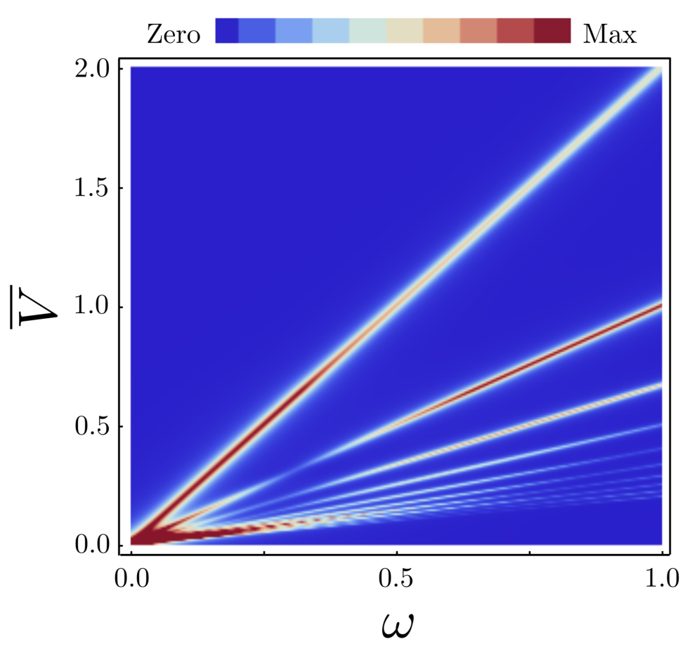
The Fourier transform of Eq. (8) is proportional to the emission spectrum of the voltage, and has been measured in Ref. 20. Performing the Fourier transform of Eq. (8), we obtain
| (9) |
where the delta function makes finite for , with () giving the fractional (integer) frequency (). Here, we have made use of the relation .
In Fig. 6 we represent as a function of and . We will focus on the two top resonance lines, which correspond from top to bottom to the frequencies (, i.e. ) and (, i.e. ), respectively. We can observe that the fractional contribution with [] dominates over the -contribution with [] for low values of . Increasing further , this tendency is reversed and the -contribution dominates. As we explained above, this can be understood in terms of the ratio , which decreases as a function of , as it was shown in Fig. 3(c) (note that is tuned by ).
For simplicity, we analyze the limit where , which yields in our dimensionless units making the second term in Eq. (9) negligible. In this scenario, the coefficient rules the periodicity of the voltage. In the limit where , , and the Fourier expansion contains only one frequency, i.e. and its harmonics. Therefore, the junction behaves like a pure -periodic junction. In the opposite limit where , the arguments , thus, Eq. (9) only contains even terms, and thus, the frequency is doubled to , yielding a contribution. This transition is shown in Fig. 6 and is consistent with the emission spectrum experiment performed in Ref. 20. The value of at which the integer contribution overcomes the fractional contribution depends only on the ratio . Thus, a direct comparison with the experimental results provides the value .[20]
IV.1.2 First-order contribution in : Shapiro steps width
The first order contribution is obtained from the solution of the linear differential equation
| (10) |
which can be solved using the integrating factor . At this point it is particularly useful to realize that
| (11) |
This relation simplifies greatly Eq. (10), yielding
| (12) |
In order to extract the width of the first two Shapiro steps we need to find the value of that makes , that is, , where . This involves the cancellation of the constant terms in the integrand of Eq. (12). The rest of the terms are canceled by the factor . Thus, when we find the equality
| (13) |
where are the Fourier coefficients of , namely,
| (14) |
The solution for corresponds to the second step , while for to the first step . The step width is given by the equation
| (15) |
Note that in pure 2-junctions the first order contribution only contains solutions for the first step width. In turn, when both contributions are present, the first-order contribution provides the width of the first and the second steps. In Fig. 7 we show the value of (the step width) as a function of . We can observe that the second step dominates for low values of , and decreases at higher values. This behavior is rather similar to the one observed in the power spectrum, where for , the fractional signal is more visible. Therefore, we can establish the connection between the periodicity of the Shapiro experiment and the radiated power spectrum observed in Refs. 17, 18, 19, 20, since we see from Eq. (15) that the Shapiro steps are proportional to the Fourier transform of .
IV.2 High intensity limit:
In this limit the zeroth-order contribution is obtained neglecting the supercurrent contributions, thus
| (16) |
where is the zeroth contribution, in units of . Eq. (16) can be integrated exactly,
| (17) |
where is a constant phase that needs to be determined, see below. Since we have linearized the differential equation, the average voltage at zeroth order is . In order to recover the Shapiro steps we need to take into account the first order contribution, given by
| (18) |
can be explicitly written by plugging Eq. (17) into Eq. (18), and taking the Jacobi-Anger expansion,
| (19) |
where is the -th Bessel function. The time average of Eq. (19) is finite for , namely
| (20) |
Shapiro steps arise choosing the value of that compensates the increment of , and thus for different values of . Therefore, the step widths will be given by the extreme value of Eq. (19) in respect to for the interval . Under these approximations, odd and even Shapiro steps are given by
| (21) |
| (22) |
where is the th-step width given in units of . In Fig. 8 we represent for and as a function of . It is important to note that both terms and enter in the same way in the step widths. Therefore, even steps can only dominate for . Furthermore, we observe in Fig. 8 a genuine oscillatory pattern. Odd step widths show a typical oscillatory pattern, i.e. they involve only one Bessel function and thus, they go to zero for given values of the argument . In turn, the even step widths are composed by the sum of two different Bessel functions. Thus, the step widths show two minima, and none of them reaches zero. Therefore, although the even step widths are comparable with the odd step widths, the beating pattern of the step widths can be used to identify and estimate the intensity of the component of the supercurrent.
V Conclusions
In this paper we study the dynamics of a Josephson junction carrying two superconducting contributions: a - and a -periodic in phase difference, with intensity and , respectively. We use the 2S-RSJ model to understand the relation between the dynamics of the junction and the width of the Shapiro steps, and in particular we focus on the reasons that make the even steps dominate over the odd steps for a fixed ratio . This phenomenon [31] is important because it has been observed in different experiments[17, 18, 20], and could help to determine the presence of topological superconductivity.
We provide a qualitative explanation of this phenomenon in terms of the washboard potential, and obtain a phase diagram of the widths of the Shapiro steps as a function of and . Remarkably, using some elementary reasonings we find the range of AC-bias, i.e. , where the non-linear dynamics of the junction causes a regime in which the even steps dominate over the odd steps. Increasing further we expect to find a crossover to a situation where odd steps are present although even steps dominate. Then, at very high values of , both contributions become comparable.
Furthermore, we study analytically the Shapiro step width as a function of in two different limits of : the low intensity limit , and the high intensity limit . The low intensity limit is precisely the limit where one can find only even Shapiro steps even when . In this limit, we find the link between two different experiments: the Josephson emission spectrum[20] and the Shapiro experiment.[17, 18, 19] In addition, we obtain analytical expressions for the step widths in the high intensity limit . We show that the maximum width of the even and odd Shapiro steps depends linearly on the ratio of . However, even in this regime one can unravel the existence of the -periodic contribution, due to the beating pattern of even Shapiro steps as a function of .

Acknowledgements.
We acknowledge financial support from the DFG via SFB 1170 ”ToCoTronics”, the Land of Bavaria (Institute for Topological Insulators and the Elitenetzwerk Bayern), the German Research Foundation DFG (SPP 1666), the European Research Council (advanced grant project 3-TOP), the Helmholtz Association (VITI) and the Spain’s MINECO through Grant No. MAT2014-58241-P. T.M.K. is financially supported by the European Research Council Advanced grant No.339306 (METIQUM) and by the Ministry of Education and Science of the Russian Federation under Contract No.14.B25.31.007. T.M.K., E.B. and L.W.M. gratefully thank the Alexander von Humboldt foundation for a Research-prize. R.S.D. acknowledges support from Grants-in-Aid for Young Scientists B (No. 26790008) and Grants-in-Aid for Scientific Research A (No. 16H02204). We acknowledge enlightening discussions with Y. V. Nazarov, J. Picó, C. Brüne and H. Buhmann.Appendix A Adapting the 2 solution to the mixed situation
The solution of Eq. (5) with and has been solved previously in Ref. 40,
| (23) |
The corresponding frequency is proportional to the voltage. Besides, the stationary voltage is equal to the frequency . In this case the time evolution of can be solved exactly and is given by
| (24) |
for . In order to adapt this solution to the more general case, where , we need to take into account the two periods and , and also to include the different intensities observed in the maxima and (see Fig. 3a). To this aim, we double the period of the system by substituting by , with , and then shift the cosine term in two opposite directions . In this way we tune from a solution that exhibits equally time spaced peaks, where the period is given by Eq. (23), to a function exhibiting peaks separated by and . In order to include two periods and mantaining the same height one needs to renormalize the Fourier coefficients and substitute by its square root of , yielding
| (25) |
This equation gives rise to peaks exhibiting equal height, in order to adjust to the numerical solution, we multiply the second term in the sum by , which in the pure solution was equal to 1, namely
| (26) |
We find that the equation becomes more similar to the numerical results when we substitute the first coefficient by 2, that is, , yielding the result given in Eq. (8). In Fig. 9 we show how accurate the approximate solution is, by comparing it against the numerical result.
References
- [1] N. Read and D. Green, Phys. Rev. B 61, 10267 (2000).
- [2] D. A. Ivanov, Phys. Rev. Lett. 86, 268 (2001).
- [3] X.-L. Qi and S.-C. Zhang, Rev. Mod. Phys. 83, 1057 (2011).
- [4] A. Nayak, S. H. Simon, A. Stern, M. Friedman, and S. D. Sarma, Phys. Rev. Mod. 80, 1083 (2008).
- [5] J. Alicea, Y. Oreg, G. Refael, F. von Oppen, and M. P. A. Fisher, Nat. Phys. 7, 412 (2011).
- [6] J. Alicea, Rep. Prog. Phys. 75, 076501 (2012).
- [7] A. Stern and N. H. Lindner, Science 339, 1179 (2013).
- [8] A. P. Mackenzie and Y. Maeno, Rev. Mod. Phys. 75, 657 (2003).
- [9] L. Elster, C. Platt, R. Thomale, W. Hanke, and E. M. Hankiewicz, Nat. Comm. 6, 8232 (2015).
- [10] A. Y. Kitaev, Phys. Usp. 44, 131 (2001).
- [11] L. Fu and C. L. Kane, Phys. Rev. B 79, 161408(R) (2009).
- [12] R. M. Lutchyn, J. D. Sau, and S. D. Sarma, Phys. Rev. Lett. 105, 077001 (2010).
- [13] Y. Oreg, G. Refael, and F. von Oppen, Phys. Rev. Lett. 105, 177002 (2010).
- [14] V. Mourik, K. Zuo, S. M. Frolov, S. R. Plissard, E. P. A. M. Bakkers, and L. P. Kouwenhoven, Science 336, 1003 (2012).
- [15] A. Das, Y. Ronen, Y. Most, Y. Oreg, M. Heiblum, and H. Shtrikman, Nat Phys 8, 887 (2012).
- [16] S. M. Albrecht, A. P. Higginbotham, M. Madsen, F. Kuemmeth, T. S. Jespersen, J. Nygård, P. Krogstrup, and C. M. Marcus, Nature 531, 206 (2016).
- [17] L. P. Rokhinson, X. Liu, and J. K. Furdyna, Nat. Phys. 1038, 2429 (2012).
- [18] J. Wiedenmann, E. Bocquillon, R. S. Deacon, S. Hartinger, O. Herrmann, T. M. Klapwijk, L. Maier, C. Ames, C. Brüne, C. Gould, A. Oiwa, K. Ishibashi, S. Tarucha, H. Buhmann, and L. W. Molenkamp, Nature Communications 7, 10303 (2016).
- [19] E. Bocquillon, R. S. Deacon, J. Wiedenmann, P. Leubner, T. M. Klapwijk, C. Brüne, K. Ishibashi, H. Buhmann, and L. W. Molenkamp, Nat. Nano. (2016), 10.1038/nnano.2016.159.
- [20] R. S. Deacon, J. Wiedenmann, E. Bocquillon, F. Domínguez, T. M. Klapwijk, P. Leubner, C. Brüne, E. M. Hankiewicz, S. Tarucha, K. Ishibashi, H. Buhmann, and L. W. Molenkamp, arXiv:1603.09611 (2016).
- [21] H. J. Kwon, K. Sengupta, and V. M. Yakovenko, Eur. Phys. J. B 37, 349 (2004).
- [22] C. W. J. Beenakker, J. M. Edge, J. P. Dahlhaus, D. I. Pikulin, S. Mi, and M. Wimmer, Phys. Rev. Lett. 111, 037001 (2013).
- [23] F. Crépin and B. Trauzettel, Phys. Rev. Lett. 112, 077002 (2014).
- [24] S. Shapiro, Phys. Rev. Lett. 11, 80 (1963).
- [25] J. C. Budich, S. Walter, and B. Trauzettel, Phys. Rev. B 85, 121405 (2012).
- [26] D. Rainis and D. Loss, Phys. Rev. B 85, 174533 (2012).
- [27] B. van Heck, F. Hassler, A. R. Akhmerov, and C. W. J. Beenakker, Phys. Rev. B 84, 180502(R) (2011).
- [28] D. M. Badiane, M. Houzet, and J. S. Meyer, Phys. Rev. Lett. 107, 177002 (2011).
- [29] P. San-Jose, E. Prada, and R. Aguado, Phys. Rev. Lett. 108, 257001 (2012).
- [30] D. I. Pikulin and Y. V. Nazarov, Phys. Rev. B 86, 140504(R) (2012).
- [31] F. Domínguez, F. Hassler, and G. Platero, Phys. Rev B 86, 140503(R) (2012).
- [32] P. Virtanen and P. Recher, Phys. Rev. B 88, 144507 (2013).
- [33] P. San-Jose, J. Cayao, E. Prada, and R. Aguado, New J. Phys. 15, 075019 (2013).
- [34] G. Tkachov and E. M. Hankiewicz, Phys. Rev. B 88, 075401 (2013).
- [35] I. Sochnikov, L. Maier, C. A. Watson, J. R. Kirtley, C. Gould, G. Tkachov, E. M. Hankiewicz, C. Brüne, H. Buhmann, L. W. Molenkamp, and K. A. Moler, Phys. Rev. Lett. 114, 066801 (2015).
- [36] B. Sothmann and E. M. Hankiewicz, Phys. Rev. B 94, 081407 (2016).
- [37] Y. M. Ivanchenko, JETP 24, 225 (1967).
- [38] W. C. Stewart, App. Phys. Lett. 12, 277 (1968).
- [39] D. E. McCumber, J. App. Phys. 39, 3113 (1968).
- [40] L. G. Aslamazov and A. I. Larkin, JETP 9, 87 (1969).
- [41] E. D. Thompson, J. Appl. Phys. 44, 5587 (1973).