Anomalous diffusion in run and tumble motion
Abstract
A random walk scheme, consisting of alternating phases of regular Brownian motion and Lévy-walks, is proposed as a model for run-and-tumble bacterial motion. Within the continuous-time random walk approach we obtain the long-time and short-time behavior of the mean squared displacement of the walker as depending on the properties of dwelling time distribution in each phase. Depending on these distributions, normal diffusion, superdiffusion and ballistic spreading may arise.
pacs
05.40-a,05.45-aWe propose a qualitative model for the movement of motile bacteria like E. Coli. These organisms have several flagella, by which they are propelled. The motion of E. Coli can be subdivided in two different phases: tumble- and run-mode. In the tumbling-mode the flagella rotate in different directions, causing an erratic movement and a fast change of orientation. In the run-mode all flagella rotate in the same direction and entangle, resulting in a straight forward movement with a constant velocity. The bacteria use the tumbling phase for chemotaxis, swimming in the direction of nutrients or away from poisonous areas. The whole process is described for instance in [1] and its numerical and theoretical description is a subject of recent discussion, see e.g. [2, 3, 4].
Random walks are the model of choice in description of motion of living organisms [1, 2, 4, 5]. Run and tumble motion is often described either by a Lévy-walk or a continuous time random walk (CTRW), also called “velocity” and “jumping process” [2]. CTRWs describe a random process consisting in instantaneous jumps separated by periods of rest (waiting times) following a given probability distribution as first discussed in [6]. A Lévy-walk is a motion at a constant speed where the direction of velocity is changed after random epochs [7]. It is essentially a CTRW in which the waiting period corresponds to a motion with constant velocity and jumps lead to a change of the direction of motion. Although Lévy-walks are commonly used to describe the (random) motion of bacteria, the origin of this kind of motion is a topic of recent studies (see e.g. [8]).
In this paper we combine both processes and model the run-and-tumble motion as an alternating random walk consisting of phases of simple diffusion (tumble phase) and of Lévy walk (run phase). A sketch of the overall process is shown in Figure 1. The speed of motion in the run phase will be denoted by and the diffusion coefficient in the tumbling phase by . The dwelling time in each phase is given by waiting time probability density functions (PDFs) and for the tumbling and run phases, respectively. All other properties in the run and tumbling phases will be denoted by subscripts and in what follows. The whole motion takes place in the space of dimensions, with or . For the sake of simplicity, we assume that the observation starts at a beginning of a run or of a tumble phase (in order to avoid the discussion of aging effects). Although the alternating setup is not a new process in the theory of random walks, and the general discussion follows the standard lines (see [9]), the model discussed below is new and far from being trivial.

The displacements in a tumbling phase are given by the transition probability density of Brownian motion
| (1) |
It depends on the time the walker has spent in this phase. Respectively, if is the elapsed time in the run phase, the transition probability density for a walk over distance reads:
| (2) |
Here is the (hyper)surface of a -dimensional unit ball which is given by: , with being the Gamma function. The corresponding probability densities are isotropic as long as no chemotactic effects are included.
We discuss the properties of the propagator of the complete process starting at and stopped (observed) at time , and concentrate on the mean square displacement (MSD)
| (3) |
Typically, the MSD follows a power law pattern, ; the value corresponds to normal diffusion and cases with to superdiffusion. The special limit is referred to as ballistic spreading. Subdiffusion, with , is impossible in our setting. Since our situation is homogeneous both in space and in time, it is easier to use the Fourier representation for the coordinate and the Laplace representation for time in which is given by an algebraic expression.
Typically, the process is stopped not at a time it changes the phase. Hence, we need two additional transition probability densities, which are
| (4) |
They describe the displacement in a prematurely finished phase (). The integral in this expression gives the probability that the dwelling time in phase exceeds . Its Laplace transform is . Thus, the are the complete analogons to the regular CTRWs waiting time PDFs after the last jump. Eq. (4) takes into account the fact that the walker continuously moves during the waiting period.
Let us assume that walks start with the beginning of a tumble phase. To find the propagator, we note that the corresponding process may have completed some number of full tumble and run cycles before the observation at time took place, and that the time is stopped either during the tumble or during the following run phase of the last, incomplete, cycle. A propagator corresponding to a full cycle is simply a convolution of and . In a Fourier-Laplace domain transforms to . The Fourier-Laplace representation of the propagator for completed cycles is given by . The remaining last cycle can be stopped either in the tumble phase or in the run phase. In the first case, the joint PDF of displacement and time in this last phase will be given by , or, in the Fourier-Laplace representation, by . If the incomplete cycle finishes in the run phase, this PDF is given by the convolution of and , corresponding to in the Fourier-Laplace representation. Summing up all the possibilities, we get
| (5) | ||||
yielding for walkers starting with a tumbling phase
Since the walker could have started in both phases, we average over the two possibilities. The averaged propagator reads
| (6) |
where we have omitted the arguments of the corresponding functions. Due to its symmetry, this expression is easier to handle and will be used for the further analysis.
The MSD in the Laplace domain is given by
| (7) |
where denotes the Laplacian in the Fourier space. To relate this MSD to the PDFs of the waiting times and to the transition probabilities, we perform explicitly the Fourier-Laplace transforms of and . It gives in case of tumbling:
where is the Laplace representation of . The same procedure applied to gives
| (8) |
Let us now turn to the Lévy walk phase. It reads
| (9) | ||||
Performing integration in we obtain
| (10) |
Here denotes the hypersurface of a -dimensional unit ball, and is an unit vector defining the point on this surface. Integration in corresponds in to the angle-integration or over the solid angle. Analogously,
| (11) |
Evaluating the Laplacian of the propagator one obtains a lengthy expression involving , and their first and second partial derivatives taken at . All items are expressed through and their first and second derivatives with respect to their argument. For the running phase, they have additionally to be integrated over the surface of the unit ball. All first derivatives of and vanish due to spacial symmetry. Terms containing a second derivative of enter expressions for and for with opposite signs and cancel. The compact final result consists of two parts corresponding to the running and the tumbling phase. It reads:
| (12) | ||||
where the derivative is taken with respect to the Laplace-variable .
Exponential Waiting Time PDFs. We now proceed by making specific assumptions about the waiting time PDFs . We first assume that all waiting time PDFs take exponential forms so that with being mean dwelling times in the corresponding phases. By plugging these expressions into (12), we can get an expression for the second moment in the spectral domain
| (13) | ||||
and from that, the asymptotic scaling in the time domain
| (14) | ||||
| (15) |
In order to obtain this result, we used Tauberian theorems, which state that the small limit corresponds to a large limit in original domain and vice versa. In both limits and , one observes normal diffusion, albeit with different diffusion coefficients.
Power Law PDFs. We will now consider waiting time distributions asymptotically following power laws for : and . Interesting new features arise if and . If the exponents are equal or larger than unity, the first moments of the waiting times are finite but the second ones diverge. If the exponents are less than unity, i.e. , even the means do not exist. As we proceed to show, the diffusive behavior is governed by the first non-analytic term of , resp. .
Let us first discuss the case when the first moments of both dwelling time distributions diverge. The corresponding expansions of the Laplace-transforms in the limit read
| (16) | ||||
| (17) |
with . In this case Eq.(12) gives in the leading order
| (18) |
Remarkably, this asymptotic expression does not explicitly depend on the diffusion coefficient of the tumbling phase. Transformed back to the time domain, the diffusive scaling depends on the relation between and :
| (19) |
Hence, we obtain superdiffusion in the long-time limit, which is always ballistic for . It is independent on the properties of the tumbling phase for , and depends on a prefactors and if . The first two regimes are dominated by Lévy walks. The third superdiffusive one with is close to a sequence of Lévy walks interrupted by rests. The tumbling periods hardly contribute to the displacement, and, therefore, a dependence on is still absent.
As one can see, the asymptotic expressions (19) fail for . In this case, subleading orders in Eqs.(17) must be taken into account. With , the Laplace transform of the waiting time density in the run phase reads
| (20) |
stands for the finite mean waiting time in this phase. The case leads to logarithmic corrections, which do not change the qualitative behaviour. We now consider the case when the first moment of the dwelling time in the run phase does exist, but the second one diverges except for the limiting value . Again we let for the tumble phase. Repeating the procedure, we get
| (21) |
wherein an explicit dependence on appears. The behavior in the time domain depends on relation between and :
| (22) |
If , the behavior of the walker still corresponds to superdiffusion, and the -dependence is suppressed. This case again is similar to Lévy walks interrupted by rests where the tumbling does not contribute to the displacement. In the two following situations with , the walker exhibits a normal diffusive behavior. In the last one with , the MSD is dominated by the random motion in the tumbling phase. The running phase has no effect on the value of the diffusion coefficient. For short times the motion is always dominated by normal diffusion.
In the limit the PDF of waiting times in the tumbling phase gets a finite first moment. The corresponding scalings are obtained from Eqs. (19) and (22). If , i.e. if the waiting times in the run phase do not possess neither a first nor a second moment, the motion is ballistic. With growing the motion tends to a superdiffusive one. The special limit is when and corresponds to the purely diffusive case. Then does possess the first moment corresponding to in the expansion (17) and does possess the second moment with value expressed by in the Laplace transform (17). The MSD can be obtained from the expression (21) by taking now into account the contribution of the second term in the denominator. This result coincides in the long time asymptotics with the one for the exponentially distributed waiting times Eq.(15).
We have seen that by choosing proper waiting time distributions of an alternating CTRW process as described above one can describe different propagation regimes in the long-time limit ranging from normal diffusion up to ballistic spreading. In the case of power-law waiting time PDFs normal diffusive behavior can only be achieved if the distribution for the Brownian part has a heavier tail than the one for runs (), which has to possess a first moment, i.e. the PDF of the Brownian tumbling phase has to have significantly more mass in the tail than its Lévy-counterpart. Such power-law-like behavior of a waiting time distribution is no rarity and occurs in several other (particularly biological) contexts [10].
We therefore expect a transition from normal to superdiffusion in cases with or with . Fig. 2 shows what diffusive regime may be expected for different values of and .
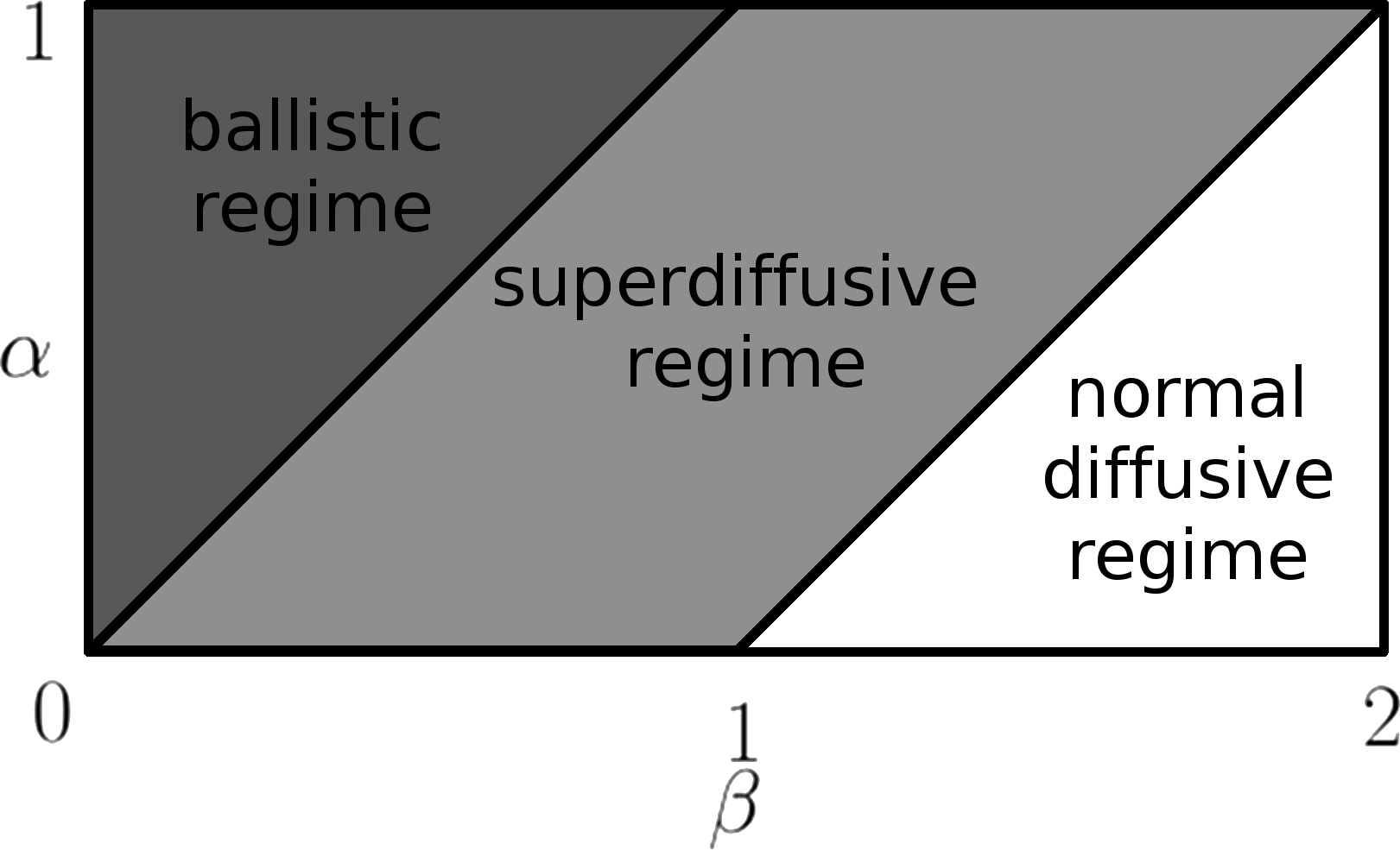
We note that if the observation does not start at time of a phase change, the model with the considered power-law distributed waiting times shows aging effects [9]. It may result in changes of prefactors in the corresponding asymptotic expressions but won’t lead to different asymptotics, so that the classification given in Fig. 2 still will hold true.
Let us summarize our findings. We proposed a phenomenological model for bacteria performing a run-and-tumble motion in the absence of chemotaxis. We have determined the possible diffusive regimes of such motion. Depending on the distribution of times in the two phases of motion, the model shows transitions from normal diffusive to superdiffusive and to ballistic behavior. Our model may prove to be useful to model situations that exhibit such transitions, such as the one described in [11]. It also may be suitable to describe non-biological situations like the motion of nanorods, which may also exhibit superdiffusion [12, 13].
The authors acknowledge financial support by DFG within IRTG 1740 research and training group project.
References
- [1] H. C. Berg, E. Coli in Motion (Springer, Heidelberg, 2004).
- [2] H. G. Othmer, S.R. Dunbar, and W. Alt, J. Math. Biol. 26, 263 (1988).
- [3] A. W. Visser and U.H. Thygesen, J. Plankton Res. 25, 1157 (2003).
- [4] D. V. Nicolau Jr., J. P. Armitage, and P. K. Maini, Comput. Biol. Chem. 33, 269 (2009).
- [5] F. J. R. Meysman, V. S. Malyuga, B. P. Boudreau, and J. J. Middelburg, Geochim. Cosmochim. Ac. 72, 3460 (2008).
- [6] E. W. Montroll and G. H. Weiss, J. Math. Phys. 6, 167 (1965).
- [7] M. F. Shlesinger, B. J. West, and J. Klafter, Phys. Rev. Lett. 58, 1100 (1987).
- [8] F. Matthäus, M. Jagodič, and J. Dobnikar, Biophys. J. 97, 946 (2009).
- [9] J. Klafter and I. M. Sokolov, First steps in random walks, 1st ed. (Oxford UP, 2011).
- [10] J. Mejias, H. J. Kappen, and J. J. Torres, PLoS ONE 5, e13651 (2010).
- [11] C. Metzner, C. Raupach, D. Paranhos Zitterbart, and B. Fabry, Phys. Rev. E 76, 021925 (2007).
- [12] D. Campos and V. Méndez, J. Chem. Phys. 130, 134711 (2009).
- [13] R. Golestanian, Phys. Rev. Lett. 102, 188305 (2009).