Identifying Key Cyber-Physical Terrain (Extended Version)
Abstract
The high mobility of Army tactical networks, combined with their close proximity to hostile actors, elevates the risks associated with short-range network attacks. The connectivity model for such short range connections under active operations is extremely fluid, and highly dependent upon the physical space within which the element is operating, as well as the patterns of movement within that space. To handle these dependencies, we introduce the notion of “key cyber-physical terrain”: locations within an area of operations that allow for effective control over the spread of proximity-dependent malware in a mobile tactical network, even as the elements of that network are in constant motion with an unpredictable pattern of node-to-node connectivity. We provide an analysis of movement models and approximation strategies for finding such critical nodes, and demonstrate via simulation that we can identify such key cyber-physical terrain quickly and effectively.
1 Introduction
1.1 Motivation
Army tactical networks in the field face a unique set of security considerations not found in either more conventional wireless networks or fixed infrastructure networks. While much previous work in analyzing the spread of malware in networks (including tactical networks) focuses on the logical connectivity of the graph over time, these logical connectivity paths are often dominated by long-range tactical links which introduce some degree of stability to the logical connectivity graph. However the close proximity of Army tactical networks to adversarial networks introduces new considerations in the form of spatial properties of the network: which units are in close proximity to each other and at what times. This form of connectivity is particularly relevant in the case of attacks that restrict themselves to short-range wireless communications – such as through 802.11 or Bluetooth network stacks – which may be more difficult to detect due to their failure to cross more conventional security boundaries or higher-resource nodes capable of fielding more sophisticated intrusion detection systems.
The short range of these attacks means that – at any given instant – the communications graph available to the malware is effectively disconnected, and it is only the mobility of the infected components over time that brings new victims into range and allows it to propagate. In addition, detection or remediation of such infections may be prohibitively difficult to perform in the field, perhaps involving detailed scans, or simply complete reimaging or replacement of any potentially compromised devices, and so only carried out at particular locations. Furthermore, while standard defensive measures are effective against known malware and minor variants, novel (“zero-day”) attacks may be specifically developed for and deployed against military mobile networks. This malware may not be detectable, and so understanding how to bound the potential impact of such malware, even when not specifically alerted to its presence, is an important problem.
The notion of mobility over time, combined with the regularities in deployment and mobility of individual Army components (such as regular patrols, movement along roads and highways, and so forth), and limited capabilities to detect or remediate such attacks, leads us to our notion of key cyber-physical terrain: critical points in the spatio-temporal graph which can be exploited to limit the spread of short-range malware. Identifying such critical points turns out to be surprisingly difficult in practice and so we explore several methods – from simple graph-theoretic approaches to dynamical system approximations to full simulation – that capture different aspects of this problem.
1.2 Related Work
Mathematical models of virus spread were first developed in the context of biological epidemics, primarily compartmental models which assume homogeneous interaction rates within the population, such as the well-known SIR (Susceptible-Infected-Recovered) model [7] and its numerous variants. Kephart and White apply compartmental models to study the dynamics of malware spread in cyber networks, additionally using simulation to evaluate under which assumptions the compartmental models are most accurate [6]. They consider several network topologies, such as Erdos-Renyi random graphs, connected regular graphs, and sparse graphs with a high clustering coefficient. In all of these topological models they study the number of infected nodes in the population over time and how various factors affect convergence to a steady state, finding that in many cases there exists a sharp epidemic threshold. Others have extended such models to additional network topologies and contexts. For example, Boguna et al. [1] and Dezső et al. [3] focus on epidemic models for power-law networks.
Marvel et al. propose a framework to evaluate cyber agility, but they focus on scenarios in which either a specific vulnerability or infected node is known to exist, and attempt to optimize the patching and isolation process in the network to preserve network integrity under various constraints including connectivity and power usage [8]. Huber et al. examine a similar problem using a decision support system in a small network of 10 active nodes [5]. Both cases assume malware with complete access to the network stack, which both allows longer-distance propagation than the local model we consider, and significantly increases the probability that the adversary will be detected.
Mickens et al. study device-to-device spreading of malicious software in mobile ad-hoc networks (MANETs) by explicitly modeling node mobility [9, 10]. Valler et al. develop a framework for analyzing malware spread in MANETs under the SIS (Susceptible-Infected-Susceptible) model [13]. Su et al. perform simulations using trace data drawn from real-life sampling of over 10,000 devices in a commuter train station to examine the propagation dynamics of Bluetooth worms, showing that Bluetooth worms can infect a large population of vulnerable devices relatively quickly in an urban environment [11]. On the other hand, Wang et al. model the spread of malware across networks of mobile phone users and observe that Bluetooth-based malware spreads slowly due to the short range of Bluetooth and therefore the relatively low contact rate between devices [14]. This highlights the fact that the dynamics of malware spread in MANETs varies significantly based on the properties of the underlying movement patterns. In particular, the highly-structured movement often seen in military contexts differentiates mobile tactical networks from civil MANETs and impacts the propagation of malware in such settings [12]. In this work, we explore how to leverage the structured mobility patterns of mobile tactical networks to develop more effective defense strategies, modeling tactical operations over a geographical region containing towns connected by a road network, and proposing computational methods to determine how to best allocate defensive resources.
1.3 Contributions and Outline
The main contributions of this work are:
- •
Model and problem formulation highlighting the need for improved security in cyber-physical tactical operations
- •
Three computational approaches for deciding where to place remediation stations to best control the spread of malware
- •
Evaluation and comparison of the three approaches
In Section 2 we describe our tactical model and propose three computational approaches to determine the optimal defender strategy. In Section 3 we perform experiments to evaluate and compare the effectiveness of the approaches. We conclude with some discussion and directions for future work in Section 4.
2 Methods
2.1 Model and Problem Statement
We consider a scenario in which tactical units of soldiers are deployed to towns in the same geographical region, connected by a road network. As time goes on, a unit may get redeployed to another town, at which point it travels from its current town to the designated town through the road network.
Each soldier is equipped with a mobile device that facilitates short-range wireless communication, such as Bluetooth, on the battlefield. Each device regularly scans the environment for nearby friendly devices. When two friendly devices come within communication range, they automatically connect, enabling data transmission.
Enemy forces may attempt to infiltrate the allied cyber network by infecting allied devices with self-propagating malware, for example by infecting the device of a captured soldier or by deploying cyber hacking teams that can infect allied devices remotely. When a soldier with an infected device comes within range of a friendly soldier with an uninfected device, the malware spreads. The malware could, for example, give the enemy access to sensitive information, or the capability to corrupt data on infected devices.
To protect their cyber network from attack, allied forces may establish some towns as remediation zones; any allied units entering such towns pass through a checkpoint where their devices are reset, replaced, or otherwise cleaned of malware. However, resources are limited, so judiciously choosing locations at which to establish remediation zones is critical.
Objective: Given knowledge of the road network, situational awareness of the location of enemy strongholds, and an assessment of remediation resources currently available, determine the optimal placement of remediation zones to minimize the fraction of devices that are infected with malware.
Below, we explore three approaches to addressing this problem: centrality analysis, dynamical systems, and agent-based modeling.
2.2 Centrality Analysis
In the centrality-based approach, we represent the road network as a graph and use network centrality analysis to identify the towns at which to establish remediation zones. The intuition is that the most central vertices are the most important, either visited most frequently or located at important junctures. Let be an undirected graph with vertex set corresponding to the towns and edge set corresponding to the roads. A centrality metric assigns weights to the vertices in a graph based on how central they are. For a given centrality metric , we let denote the mapping from the vertices of to their corresponding values under the centrality metric.
We consider two common centrality metrics:
- •
PageRank centrality [2] - favors vertices with connections to other well-connected vertices
- •
Betweenness centrality [4] - favors vertices that lie on shortest paths between many other pairs of vertices
The choice of metric may be context-specific. For example, PageRank centrality has a natural correspondence with the frequency of vertices being visited under a mobility model where units perform a random walk on the road network, i.e. choosing the next town to visit uniformly at random from the set of neighboring towns. On the other hand, Betweenness centrality naturally corresponds with vertex frequency under a random waypoint mobility model, i.e. where units choose a town uniformly at random from the set of all towns and then traverse a shortest path to get there.

If there are only resources for a single remediation zone, centrality metrics offer a straight-forward way to choose where to place it: at the town corresponding to the vertex with the highest centrality score. If there are resources for remediation zones, however, the natural solution of choosing the towns corresponding to the vertices with the highest centrality values may not be a very good strategy. For example, consider the graph in Figure 1 with . Vertices and have the top two centrality scores for PageRank and Betweenness centrality, yet a better strategy would likely be to choose one vertex in and one vertex in because that would cut the graph into two similarly-sized subgraphs between which malware could not propagate.
Input: A graph , a centrality metric , and an integer .
Output: A subset of size corresponding to the towns at which to establish remediation zones.
- 1.
Initialize
- 2.
For :
- •
Compute
- •
Set
- •
Set
- •
- 3.
Return
To address this problem, we present an iterative algorithm, described in Algorithm 1. The algorithm computes centrality scores, deletes the vertex with the highest score, and repeats until vertices have been deleted. The remediation zones should be placed at the towns corresponding to the deleted vertices.

However, there are still times when this does not produce the desired behavior. For example, consider the graph in Figure 2 with . Vertices and are tied for the top centrality score for PageRank and Betweenness centrality. After one of them is deleted, the other still has the highest score on the remaining graph. However, a better strategy would likely be to choose vertices and for the same reason as above.

Furthermore, there is no clear way of incorporating situational awareness of which towns are controlled by the enemy and therefore most likely that allied devices will get infected with malware. For example, consider the graph in Figure 3 with . Vertex has the highest centrality score for both metrics, but the best strategy would obviously be to choose vertex . This is a drawback of any centrality-based algorithm, since they are based solely on the network topology and are not sensitive to the locations of enemy strongholds.
Next we consider an approach from the field of dynamical systems that addresses these problems.
2.3 Dynamical Systems
In the dynamical systems approach, we begin by modeling the movement of each unit as a continuous-time Markov chain, where states correspond to towns and roads, and transitions correspond to changes in location in response to new tactical orders. When deployed at a town, a unit stays there for some deployment time until it receives new orders to travel to a neighboring town. When it receives the travel order, it transitions to the road between the two towns, and remains there for the duration of the travel time, which may depend on the distance, terrain, weather conditions, etc.
Let denote the state corresponding to town , and let denote the state corresponding to traversing a road from town to town . We define the average wait time for state to be equal to the average deployment time for town . We define the average wait time for state to be equal to the average travel time from town to town .
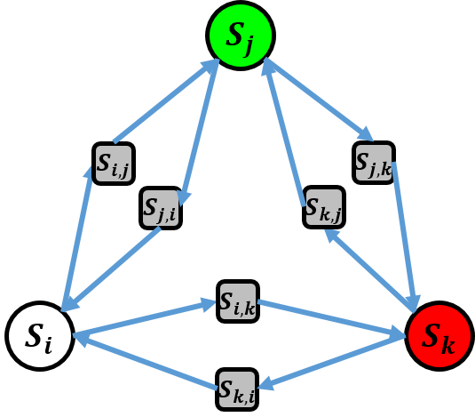
There are two types of transitions: from a state to a state , corresponding to departure from town along a road to town ; and from a state to a state , corresponding to arrival at town along a road from town . Assuming that units leaving a town have the same likelihood of traveling to each of the neighboring towns, the transition rates are as follows:
The Markov chain for a simple example scenario is illustrated in Figure 4.
Next, we describe the movement of all units collectively using a compartmental model corresponding to the Markov chain described above, capturing the fraction of units in each state and the flows between them with a set of differential equations. These equations can then be used to solve for the fraction of units in each state at equilibrium, indicating which towns will be most frequently visited, which could be good candidates for remediation zones. A more detailed technical description of this approach is provided in Appendix A.
However, the same problems encountered under the centrality-based approach above still remain: choosing a set of towns based on each town’s individual value may not yield the best results collectively; and we have not leveraged knowledge of the location of enemy strongholds.

To address these problems, we consider a modified Markov model that splits each previous state into two dual states, corresponding to whether the unit is clean or infected. We denote this by states , , , and . Let denote the set of vertices corresponding to enemy strongholds, and let denote the set of vertices corresponding to towns with remediation stations, with . We assume that any unit entering a town in will become infected with malware, and any unit entering a town in will become clean. In addition, we assume that a clean unit entering a town with at least one infected unit will become infected, and also that a clean unit traversing a road with at least one infected unit traveling in the opposite direction will become infected. The goal is to determine the optimal set of size , given . The modified Markov chain for the example scenario is illustrated in Figure 5.
Similarly to above, the movement of all units collectively can be captured by a set of differential equations, which, given and , can be solved efficiently for the equilibrium fraction of units in each state (see Appendix A for details). In this modified model, however, we have a way of quantifying the effectiveness of a proposed solution: the total fraction of infected units at equilibrium. The remaining challenge is in finding the set that minimizes that value.
Input: A graph representing towns connected by a road network, a subset of vertices corresponding to enemy strongholds, a function mapping vertex subsets to the resulting fraction of infected units if remediation zones were established at the corresponding towns, an integer indicating how many random samples to take at the corresponding point in the algorithm, and an integer indicating the number of remediation zones for which resources are available.
Output: A subset of size corresponding to the towns at which to establish remediation zones.
- 1.
Initialize
- 2.
Initialize
- 3.
Initialize
- 4.
For :
- •
For :
- –
Initialize
- –
Initialize
- –
- •
for
- –
Randomly select a subset of size
- –
Set
- –
For :
- *
Update
- *
Update
- *
- –
If :
- *
Set
- *
Set
- *
- –
- •
Set
- •
Set
- •
- 5.
Return
If , the number of towns, and , the desired number of remediation stations, are small, then an exhaustive search may be feasible. Otherwise, we propose two algorithms: one which simply entails sampling from the space of possible solutions and choosing whichever solution gives the best result; and one which is based on more sophisticated random sampling and Monte Carlo methods, described in Algorithm 2.
The dynamical systems approach addresses some of the major problems with the centrality-based approach, viz. considering multiple towns simultaneously, and explicitly representing the presence of enemy strongholds. However, it is less flexible than the centrality-based approach in accommodating different mobility models; the Markov property is fine for modeling a random walk on the road network, but cannot easily represent multi-hop paths such as traversing the shortest path between two towns. In addition, the model makes several simplifying assumptions that could compromise the accuracy of the results.
Next, we present an approach that gives greater flexibility in modeling and also permits a higher degree of realism.
2.4 Agent-based Modeling

In this approach, we develop an agent-based model to represent the movement of and interactions between tactical units. The agents are the tactical units, each represented by a Unit object. The environment consists of Town objects, represented by circular regions, and Road objects, each connecting two Towns. Towns can be ally-controlled, enemy-controlled, or neutral. This approach can accommodate many different mobility models, including both the random walk and the random waypoint models for traversing the road network. An agent-based model for a simple example scenario is illustrated in Figure 6.
When a Unit is deployed at or passes through an enemy-controlled Town, we make the worst-case assumption that the enemy will be able to infect at least one of the soldiers’ devices, and that relatively soon thereafter the malware will spread to the whole Unit as the soldiers interact with one another. In addition, we assume that if two Units are deployed to the same Town simultaneously, or if one Unit passes through the Town where the other is deployed, or if two Units pass each other on a Road, there will be at least some contact between the Units; therefore, if one of them is infected, the other will also become infected.
As before, our goal is to determine the set of vertices at which to place remediation zones so as to minimize the fraction of infected units. An obvious way to evaluate a proposed solution, then, is to run the simulation for a period of time and then count how many of the units are infected. Because of random variation, the result should be averaged over multiple trials. As with the dynamical systems approach, the remaining challenge is in finding the set that minimizes that value. For this, we propose using either the simple random sampling method or the same Monte Carlo algorithm proposed above, Algorithm 2, substituting the results of the agent-based simulation for the solution to the dynamical system when defining the function .
The agent-based modeling approach has higher fidelity and expressiveness than the other approaches, but can also be more computationally expensive. In the following section, we evaluate both the effectiveness and computational efficiency of the three methods in determining the placement of remediation stations to best limit the spread of malware.
3 Evaluation
We now perform experiments to evaluate and compare the performance of the three approaches. Since the agent-based model has the highest fidelity of the three approaches, we use it as an evaluative metric to compare different recommended placement strategies. Given that, one might expect that the agent-based modeling approach would trivially yield the best results. However, as we will observe, due to computational limitations this is not always the case.
Before we proceed with the experiments, we provide details of our implementation.
3.1 Implementation and Experimental Setup
All three of the approaches are implemented in Java. Solving systems of equations for the dynamical systems approach was done using the JAMA linear algebra package. Simulations of the agent-based model can be visualized using Repast Simphony, a Java-based agent-based modeling and simulation environment. Experiments are conducted on an Intel Core i7 processor operating at 2.40 GHz with 16 GB of memory running Windows 10.

Figure 7 gives a screenshot of an example run of the agent-based simulation. The black circles represent neutral Towns, the red circles represent Towns under enemy control, and the green circles represent Towns under allied control. Units are depicted by a red ‘X’ when infected and a black ‘X’ when uninfected.
For the experiments presented here, we consider five tactical units operating in a geographical area consisting of 35 towns connected by a road network. Units move at a speed of 10 m/s, and deployments last 2 hours. We vary the number of infected towns and remediation zones. Simulations were run for 10,000 time steps. Results were averaged over 20 independent trials.
3.2 Results
| # Inf Zones | # Rmd Zones | Betweenness | PageRank | Dynam Sys | Agent-based | Uniform Random | ||||
|---|---|---|---|---|---|---|---|---|---|---|
| Top-k | Iter | Top-k | Iter | Basic | MC | Basic | MC | |||
| 5 | 0 | 1.000 | 1.000 | 1.000 | 1.000 | 1.000 | 1.000 | 1.000 | 1.000 | 1.000 |
| 5 | 1 | 0.844 | 0.834 | 0.861 | 0.844 | 0.795 | 0.795 | 0.870 | 0.870 | 0.862 |
| 5 | 3 | 0.701 | 0.710 | 0.658 | 0.582 | 0.572 | 0.573 | 0.675 | 0.640 | 0.716 |
| 5 | 5 | 0.615 | 0.618 | 0.514 | 0.438 | 0.442 | 0.424 | 0.541 | 0.515 | 0.594 |
| 3 | 5 | 0.480 | 0.529 | 0.407 | 0.295 | 0.336 | 0.274 | 0.445 | 0.393 | 0.493 |
| 1 | 5 | 0.199 | 0.248 | 0.186 | 0.113 | 0.128 | 0.101 | 0.197 | 0.113 | 0.267 |
| 0 | 5 | 0.000 | 0.000 | 0.000 | 0.000 | 0.000 | 0.000 | 0.000 | 0.000 | 0.000 |
| # Inf Zones | # Rmd Zones | Betweenness | PageRank | Dynam Sys | Agent-based | Uniform Random | ||||
|---|---|---|---|---|---|---|---|---|---|---|
| Top-k | Iter | Top-k | Iter | Basic | MC | Basic | MC | |||
| 5 | 0 | 1.000 | 1.000 | 1.000 | 1.000 | 1.000 | 1.000 | 1.000 | 1.000 | 1.000 |
| 5 | 1 | 0.743 | 0.793 | 0.852 | 0.743 | 0.779 | 0.779 | 0.878 | 0.878 | 0.940 |
| 5 | 3 | 0.543 | 0.673 | 0.640 | 0.446 | 0.526 | 0.556 | 0.717 | 0.621 | 0.758 |
| 5 | 5 | 0.461 | 0.581 | 0.520 | 0.345 | 0.403 | 0.395 | 0.561 | 0.489 | 0.624 |
| 3 | 5 | 0.321 | 0.474 | 0.385 | 0.203 | 0.289 | 0.238 | 0.373 | 0.312 | 0.455 |
| 1 | 5 | 0.112 | 0.252 | 0.160 | 0.068 | 0.122 | 0.096 | 0.148 | 0.088 | 0.214 |
| 0 | 5 | 0.000 | 0.000 | 0.000 | 0.000 | 0.000 | 0.000 | 0.000 | 0.000 | 0.000 |
The results of our experiments are shown in Tables 1 (Random Walk mobility model) and 2 (Random Waypoint mobility model). For a baseline, we also record the average fraction of infected units when remediation zones are chosen uniformly at random.
The best performers under the Random Walk mobility model were the Iterative PageRank Centrality method and the Dynamical Systems methods (either using simple random sampling or the more sophisticated Monte Carlo algorithm). The other methods performed significantly worse than those, and comparably to one another, sometimes not even matching the results of the uniform random baseline.
Under the more realistic Random Waypoint mobility model, Iterative PageRank was the clear winner, performing even better than under Random Walk. This was surprising, and ran counter to our intuition that PageRank would perform best under Random Walk because it has a natural correspondence to walks on graphs. Similarly, we were surprised that Betweenness centrality did not perform better under the Random Waypoint model, given its natural correspondence to graph paths. With the exception of the Iterative Betweenness method, all methods out-performed the baseline.
We note that we configured the ABM method to use fewer MC samples than the Dynamical Systems method (10 instead of 100) to keep its runtime comparable, since it does an evaluation over 10 sample trials for each candidate strategy rather than just solving a system of equations once. We suspect that the small sample size resulted in a high variance across trials, which could explain why the ABM approach performed so poorly.
| Betweenness | PageRank | Dynam Sys | Agent-based | Uniform Random | |||||
| Top-k | Iter | Top-k | Iter | Basic | MC | Basic | MC | ||
| Runtimes | 0.209 | 0.209 | 0.209 | 0.208 | 0.414 | 0.418 | 1.247 | 1.040 | 1.247 |
Runtimes are shown in Table 3. For this setting of the parameters, the centrality algorithms each ran in about 12 seconds, Dynamical Systems ran in about 25 seconds, ABM with MC in about 60 seconds, and ABM with random sampling in about 75 seconds.
4 Conclusions
| Approach | Pros | Cons |
|---|---|---|
| Centrality metrics | can be efficient, choice of metric can accommodate different contexts or mobility patterns | does not capture travel times, cannot specify enemy towns, not good for multi-site selection |
| Dynamical systems | efficient, good for multi-site selection | assumes Random Walk mobility pattern because of Markov property |
| Agent-based modeling | very flexible and expressive, most realistic, good for multi-site selection | not as efficient as other approaches |
We have proposed the notion of “key cyber-physical terrain” to describe the risk posed by short-range wireless attacks under the dynamic connectivity graphs of field operations: specific physical locations at which mobile devices can be examined and remediated to minimize the ability of an adversary to maintain a presence on the mobile network. As the exact solution to this problem is computationally intractable, we have also proposed three approximate methods of solving the associated minimization problem – centrality metrics, dynamical systems, and agent-based modeling – under two different models of unit mobility. Some of their pros and cons are listed in Table 4.
Our results suggest that the problem of malware propagating through short-range wireless communications is potentially quite significant, with a high prevalence of malware persisting on the network, even when the remediation zones are placed strategically in response to the locations of the infection zones. It is also worth noting that simple algorithms based on network centrality metrics, in particular PageRank centrality, can match and even outperform more complex approximations, even under the more realistic Random Waypoint mobility model. In either case, we obtain solutions reasonably quickly, with average runtimes of about 1 minute even for our most computationally intensive approach. We note, however, that the variance for the agent-based modeling is relatively high, as the total number of potential trajectories through the combinatorial number of remediation zones is prohibitively large; results could be improved by increasing sample sizes in the Monte Carlo algorithm, at the cost of longer runtimes, which would be further exacerbated as the problem scales up. Methods to mitigate this variance will be explored in future work.
Our current results show that both our centrality and dynamical systems methods can approach the accuracy of the more computationally intensive agent-based modeling approach under the mobility models used. On the other hand, the agent-based approach provides much greater flexibility for representing more sophisticated and realistic movement patterns and higher-fidelity models. For example, instead of random deployments and shortest-path traversals, simulations could be performed using real-world maps and scenarios, and paths may intentionally avoid locations of enemy strongholds. An alternative problem formulation could allow strategies to simultaneously define the traversal paths between pairs of towns as well as the locations of the remediation zones. This will be explored in future work, as well as extensions to our tactical model in which enemy infection regions as well as remediation zones may be dynamic or increase in number.
References
- [1] M. Boguná, R. Pastor-Satorras, A. Vespignani, et al. Epidemic spreading in complex networks with degree correlations. In Proceedings of the XVIII Sitges Conference on Statistical Mechanics, Lecture Notes in Physics, Springer, Berlin, 2003.
- [2] S. Brin and L. Page. The anatomy of a large-scale hypertextual web search engine. Computer Networks and ISDN Systems, 30(1):107 – 117, 1998.
- [3] Z. Dezső and A.-L. Barabási. Halting viruses in scale-free networks. Physical Review E, 65(5):055103, 2002.
- [4] L. C. Freeman. A set of measures of centrality based on betweenness. Sociometry, 40(1):35–41, 1977.
- [5] C. Huber, P. McDaniel, S. E. Brown, and L. Marvel. Cyber fighter associate: A decision support system for cyber agility. In 2016 Annual Conference on Information Science and Systems (CISS), pages 198–203. IEEE, 2016.
- [6] J. Kephart and S. White. Directed-graph epidemiological models of computer viruses. In Research in Security and Privacy, 1991. Proceedings., 1991 IEEE Computer Society Symposium on, pages 343–359, May 1991.
- [7] W. O. Kermack and A. G. McKendrick. A contribution to the mathematical theory of epidemics. Proceedings of the Royal Society of London A: Mathematical, Physical and Engineering Sciences, 115(772):700–721, 1927.
- [8] L. M. Marvel, S. Brown, I. Neamtiu, R. Harang, D. Harman, and B. Henz. A framework to evaluate cyber agility. In Military Communications Conference, MILCOM 2015-2015 IEEE, pages 31–36. IEEE, 2015.
- [9] J. W. Mickens and B. D. Noble. Modeling epidemic spreading in mobile environments. In Proceedings of the 4th ACM Workshop on Wireless Security, WiSe ’05, pages 77–86, New York, NY, USA, 2005. ACM.
- [10] J. W. Mickens and B. D. Noble. Analytical models for epidemics in mobile networks. In Third IEEE International Conference on Wireless and Mobile Computing, Networking and Communications (WiMob 2007), pages 77–77. IEEE, 2007.
- [11] J. Su, K. K. Chan, A. G. Miklas, K. Po, A. Akhavan, S. Saroiu, E. de Lara, and A. Goel. A preliminary investigation of worm infections in a bluetooth environment. In Proceedings of the 4th ACM Workshop on Recurring Malcode, pages 9–16. ACM, 2006.
- [12] B. Thompson and J. Morris-King. The impact of hierarchy on bluetooth-based malware spread in mobile tactical networks. In Proceedings of the Summer Computer Simulation Conference, SCSC ’16, pages 34:1–34:7, San Diego, CA, USA, 2016. Society for Computer Simulation International.
- [13] N. C. Valler, B. A. Prakash, H. Tong, M. Faloutsos, and C. Faloutsos. Epidemic spread in mobile ad hoc networks: Determining the tipping point. In Proceedings of the 10th International IFIP TC 6 Conference on Networking - Volume Part I, NETWORKING’11, pages 266–280, Berlin, Heidelberg, 2011. Springer-Verlag.
- [14] P. Wang, M. C. González, C. A. Hidalgo, and A.-L. Barabási. Understanding the spreading patterns of mobile phone viruses. Science, 324(5930):1071–1076, 2009.
Appendix A: Theoretical Analysis of the Dynamical Systems Approach
We consider tactical units moving along a road network connecting a set of towns. We represent the network as a directed graph with vertex set corresponding to the towns and edge set corresponding to the roads. Let denote the degree of vertex in , corresponding to the number of roads into town . Table 5 provides a summary of the notation used in our model.
| the number of units/companies | |
| the number of towns | |
| vertex corresponding to town | |
| edge corresponding to a road between town and town | |
| the degree of (equivalently, the number of roads into town ) | |
| state corresponding to being in town | |
| state corresponding to being on the road from to | |
| the average wait time for state (average deployment time at town ) | |
| the average wait time for state (average travel time on the road from to ) | |
| the transition matrix | |
| limiting probability of being in state | |
| limiting probability of being in state | |
| , | states corresponding to being in town and clean/infected |
| , | states corresponding to being on the road from to and clean/infected |
| , | limiting probabilities of being in states and , respectively |
| , | limiting probabilities of being in states and , respectively |
We model the movement of each unit as a continuous-time Markov chain, where states correspond to towns and roads, and transitions correspond to changes in location in response to new tactical orders. When deployed at a town, a unit stays there for some deployment time until it receives new orders to travel to a neighboring town. When it receives the travel order, it transitions to the road between the two towns, and remains there for the duration of the travel time, which may depend on the distance, terrain, weather conditions, etc.
Let denote the state corresponding to town , and let denote the state corresponding to traversing a road from town to town . We define the average wait time for state to be equal to the average deployment time for town . We define the average wait time for state to be equal to the average travel time from town to town .
Let denote the transition matrix, i.e. is the transition rate from state to state . There are two types of transitions: from a state to a state , corresponding to departure from town along a road to town ; and from a state to a state , corresponding to arrival at town along a road from town . The transition rates are as follows:
We now take a mean-field approach, modeling all units collectively using a compartmental model corresponding to the Markov chain described above. Let denote the fraction of units that are in town at time , and let denote the fraction of units that are on the road from town to town at time . We provide the master equations expressing the instantaneous rate of change for each of the compartments:
The limiting distribution over node states can be determined by solving the following system of equations, derived by setting for all states, where and are the limiting probabilities:
Since this is a system of linear equations — of which are linearly independent — in variables, it can be solved efficiently, e.g. using Gaussian elimination.
Next we consider enemy cyber hacking teams planted in some of the towns. When an allied unit gets deployed to one of those towns, the enemy cyber team hacks into a soldier’s device and infects it with a self-propagating Bluetooth worm, which then spreads to the devices of other soldiers in the unit as they continue carrying out their tactical objectives. In addition, malware then spreads from an infected unit to a clean unit when the two units are deployed in the same town at the same time, or when they pass each other on the road (going in opposite directions). We represent this with a modified Markov model that splits each previous state into two dual states, corresponding to whether the unit is clean or infected. We denote this by states , , , and . Let denote the set of vertices corresponding to towns with enemy cyber hacking teams.
For defensive strategy, we consider “cleaning stations” that may be placed at the entrance to towns. Any infected units that pass through one of the cleaning stations will become clean. Let denote the set of vertices corresponding to towns with cleaning stations. We assume that .
There are now nine types of transitions:
- •
from to , when a clean unit departs from town along a road to town , and there are currently no infected units traveling from town to town
- •
from to , when a clean unit arrives at town along a road from town , and there are currently no infected units deployed at town and no enemy cyber hacking team
- •
from to , when a clean unit departs from town along a road to town , and there is currently an infected unit traveling from town to town
- •
from to , when a clean unit arrives at town along a road from town , and there is currently an infected unit deployed at town or an enemy cyber hacking team
- •
from to , when a clean unit gets infected in a town due to the arrival of an infected unit
- •
from to , when a clean unit gets infected on a road by an infected unit starting to travel down the road in the opposite direction
- •
from to , when an infected unit departs from town along a road to town
- •
from to , when an infected unit arrives at town along a road from town , and there is not a cleaning station at town
- •
from to , when an infected unit arrives at town along a road from town , and there is a cleaning station at town
The corresponding transition rates are as follows, and :
This corresponds to a new set of master equations, also and :
Setting for all states yields the following system of equations, where , , , and are the limiting probabilities, again and :
We note that some of these equations are non-linear. However, the non-linear terms can be approximated by substituting or — whose values can be computed efficiently from the first system of equations — for each occurrence of or , respectively. This substitution over-estimates fractions of infected nodes, thus yielding a set of linear equations in the new variables , with the property that and :