Yoshikawa moves on marked graphs via Roseman’s theorem
Abstract.
Yoshikawa [Yo] conjectured that a certain set of moves on marked graph diagrams generates the isotopy relation for surface links in , and this was proved by Swenton [S] and Kearton and Kurlin [KK]. In this paper, we find another proof of this fact for the case of -links (surface links with spherical components). The proof involves a construction of marked graphs from branch-free broken surface diagrams, and a version of Roseman’s theorem [R] for branch-free broken surface diagrams of -links.
August 24, 2026
1. Introduction
For a smooth oriented manifold we denote by the group of orientation-preserving diffeomorphisms of and by the path-component of the identity in . We orient in the standard way. A surface link is a smooth submanifold diffeomorphic to a closed surface (i.e. compact with no boundary). We say two surface links and are isotopic if there is with . A -link is a surface link where each component is a -sphere. Let be the set of surface links, the set of surface links with orientable components, and the set of -links.
In Section 2 we review the definitions of generic projections, broken surface diagrams, Roseman moves, and Roseman’s theorem. We prove Theorem 2.9, a version of Roseman’s theorem for branch-free broken surface diagrams of -links, stating that two isotopic branch-free broken surface diagrams of a -link are related by a finite sequence of , , , , and moves (see Figures 3 and 7). This theorem complements the results of Takase and Tanaka [TT], who find examples of isotopic branch-free broken surface diagrams of a -link that are not related by , , and moves alone.
In Section 3 we review marked graphs in , marked graph diagrams in , Yoshikawa moves on marked graph diagrams, -surfaces obtained from marked graphs, and prove some facts about marked graphs and -surfaces. In Section 4 we describe a relationship between branch-free broken surface diagrams and -surfaces, and provide another proof that two marked graph diagrams describe isotopic -links if and only if they are related by a finite sequence of Yoshikawa moves (see Theorem 4.4).
Acknowledgements
The author wishes to thank Dror Bar-Natan, J. Scott Carter, Michał Jabłonowski, Seiichi Kamada and Vassily O. Manturov for pointing out some inaccuracies and providing helpful references and comments.
2. Broken surface diagrams and Roseman’s theorem
Definition 2.1 reviews generic projections, broken surface diagrams and Roseman moves. Roseman’s theorem is stated in Theorem 2.2. We use Lemma 2.7 to prove Theorem 2.9, a branch-free version of Roseman’s theorem.


Definition 2.1.
References for the definitions we present here can be found for example in Carter, Kamada and Saito [CKS], Kamada [Kam] and Roseman [R]. Let be the projection . If there is isotopic to such that a neighbourhood in of any point of is one of the four possibilities in Figure 1. Such a projection will be called generic.
Assume is such that is generic. Let be the set of branch, double and triple points. If is a double point then there exist with and these two points are ordered by the -coordinates of and . Similarly if is a triple point then there exist with and these three points are ordered by the -coordinates of , and . The orderings extend by continuity to neighbourhoods of the points in . The projection along with all of the above crossing information is called a broken surface diagram. Following Takase and Tanaka [TT], we refer to a broken surface diagram with no branch points as branch-free. We consider two broken surface diagrams equivalent if they differ by the action of and agree on crossing information. We may indicate the crossing information near a double-point by removing a neighbourhood of one of the pre-images with the convention that missing segments have greater -coordinates as in Figure 2. Figure 3 depicts the Roseman moves on broken surface diagrams. Appropriate crossing information should be added for completeness. The move is slightly different but equivalent modulo the and moves, to the usual move.
If is a set of surface links let be the set of broken surface diagrams corresponding to links in with generic projections, and let be the subset of branch-free broken surface diagrams.
Theorem 2.2 (Roseman [R]).
If represent isotopic surface links then and are related by a finite sequence of the moves in Figure 3 and equivalences in .


Remark 2.3.
In the paper of Bar-Natan, Fulman and Kauffman [BKF] there is a proof of the well-known fact that all spanning-surfaces of a classical link in are tube-equivalent. In that proof, link projections are used to construct Seifert surfaces via Seifert’s algorithm, and the main result is deduced by observing how the constructed Seifert surfaces change when Reidemeister moves are performed on the link projection.
We wish to approach the proofs of Theorems 2.9 and 4.4 in a similar manner. We will assign various structures (a set of branch-free broken surface diagrams in the case of Theorem 2.9 and an -surface in the case of Theorem 4.4) to a broken surface diagram and observe how these structures change when Roseman moves are performed on the broken surface diagram.
Definition 2.4.
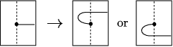
Following Carter and Saito [CS], we define a function (where is the power set of ). Let be a broken surface diagram corresponding to a generic projection for some with components . If is such that is a branch point, then a neighbourhood of looks as in Figure 4. Let be the broken surface diagram obtained from by removing all components except . Each has an equal number of positive and negative branch points, and any pair of positive and negative branch points can be cancelled using an appropriate sequence of moves followed by an move.
Specifically, assume has branch points and for and let be the distinct points such that and are positive and negative branch points in . A pair is valid if:
- -
each is a permutation of ,
- -
is a disjoint union of embedded oriented compact intervals with endpoints and the orientation going from to ,
- -
is transverse in and is embedded in ,
- -
after performing the sequence of moves pushing along through all intersections in , it is possible to perform a final move cancelling and .
The set contains a broken surface diagram for each valid pair , obtained by actually performing on the aformentioned moves along each ending in an move cancelling the branch points and . If there are no branch points in we let .
Remark 2.5.
It is important to note that the final requirement for valid paths in Definition 2.4 is not superfluous. There exist invalid collections of simple paths satisfying the first three requirements. However if a particular path satisfies the first three requirements but not the fourth, then it can be made valid by the modification in Figure 5. This is depicted on the level of broken surface diagrams in Carter and Saito [CS, Figure K and Figure M].
Remark 2.6.
Figure 6 describes moves on the valid pairs of Definition 2.4. For each move, the diagram remains fixed and the set thus remains fixed as well. The moves correspond to an isotopy of rel in , interacting with the set . The moves and describe two types of interactions of two simple paths in . The move acts as a transposition on one of the permutations in . While moves and valid pairs are somewhat adhoc objects, in Lemma 2.7 we will see that the moves correspond naturally to moves on broken surface diagrams, described in Figure 7. Note that each move does in fact represent an isotopy in , since it can be written in terms of Roseman moves, in particular and moves.


Lemma 2.7.
- a)
- b)
The , , and moves can be expressed in terms of , , , and moves.
- c)
- d)
If , , and and are related by a Roseman move then and are related by a sequence of , , , , and moves.
Proof.
- a)
Assume we have two pairs and with the same set of permutations and let and . If for some the pairs and do not agree in small enough neighbourhoods of the points and in , then they can be made to agree using a move, due to the fact that the pairs and satisfy the last property in Definition 2.4. Thus we assume for each the paths and agree in small enough neighbourhoods of the points and in . Since each component of is a sphere, there is an isotopy in taking to relative to their common boundary and . During this isotopy, does not change in a small enough neighbourhood of its boundary. Such an isotopy can be accomplished using the , , , , and moves. Thus after performing each isotopy for all choices of we get a sequence of moves taking to .
Consider now the case of two pairs and with . It is enough to assume that all permutations in agree with their respective permutations in except for some two permutations that differ by a transposition. We can induce an arbitrary transposition using a move. If we wish to perform a move between and we can use moves to bring them into the exact form in the left-hand side of the move. Now if the move is valid (i.e. lifts to the move in Figure 7), we can perform the move to induce a transposition. If the move is not valid, it can be made valid after a move along either of the paths. Thus we may induce arbitrary transpositions in the ’s using moves.
Thus the moves suffice to connect all valid pairs in Definition 2.4.
- b)
We leave it to the reader to verify that the , , and moves can be expressed in terms of , , and moves. Figure 8 expresses a move using , and moves.

Figure 8. Showing that a move can be realized with , and moves. - c)
If then by Lemma 2.7a their defining valid pairs are related by moves. The moves , , , and on valid pairs can be realized directly by the moves , , , and respectively on broken surface diagrams. The move can be realized by a sequence involving , , , and moves. The move can be realized by a sequence involving , , and moves. By Lemma 2.7b, the , , and moves can be expressed in terms of , , , and moves, so we are done.
- d)
If and are related by an , , , or move, then it is not difficult to see that there are diagrams and such that and are related by an , , , or move. By Lemma 2.7c, is related to and is related to by a sequence of , , , , and moves. Thus there is a sequence of , , , , and moves relating to .
If an move takes to then there are diagrams and with a move taking to (note that the two branch points created by the move can be paired in two obvious ways. One way can be cancelled by an move and the other can be cancelled by , and moves, similar to Figure 8). Thus by Lemma 2.7c again there is a sequence of , , , , and moves relating to .
∎
Remark 2.8.
Now we can prove a branch-free version of Roseman’s theorem.
Theorem 2.9.
If are related by a finite sequence of Roseman moves then they are related by a finite sequence of , , , , and moves.
3. Marked graphs and -surfaces
Lomonaco [L] and Yoshikawa [Yo] described another method of representing surface links via certain -regular rigid vertex graphs in . Definition 3.1 reviews marked graphs and the Yoshikawa moves on marked graph diagrams. Definition 3.2 concerns -surfaces and -moves. Definition 3.3 presents the and functions. Lemma 2.7 describes some key properties pertaining to marked graphs, -surfaces and the and functions.
Definition 3.1.
A marked graph is a -regular rigid vertex graph (with some components possibly having no vertices) where:


We consider two marked graphs equivalent if they differ by the action of in a way that preserves rigid neighbourhoods of their vertices, and have agreeing markers. Let be the set of marked graphs. One may project a marked graph to and obtain a marked graph diagram. Figure 11 describes the Yoshikawa moves on marked graph diagrams. The moves do not change the equivalence class of the marked graph in . The results in Kauffman [Kau] show that these first five moves do in fact generate the equivalence relation on marked graph diagrams coming from the action of on marked graphs in . The moves differ from moves in that they are defined for marked graphs in , not just marked graph diagrams in .

Definition 3.2.
An -surface is a compact not necessarily connected not necessarily orientable surface with boundary where:
- -
each boundary component of is assigned a label from the set ,
- -
each component of contains at least one -labelled and at least one -labelled boundary component,
- -
the -labelled and -labelled boundary links are trivial.
We consider two -surfaces equivalent if they differ by the action of and have matching labellings of their boundaries. Let be the set of -surfaces, the subset of orientable -surfaces, and the subset of orientable -surfaces in which each component has genus . We will refer to the moves on -surfaces in Figure 12 as -moves.

Definition 3.3.
The function , mapping a marked graph to an -surface up to moves, is given in Figure 13. Since this is defined locally on the edges and marked vertices of a marked graph, we must glue the final result in a way that preserves the -labels coming from marked vertices, and this can only be done up to moves. Note that and holds for any -regular rigid vertex graph that satisfies the first condition in Definition 3.1. For denote by the set of all with .

There is a function defined as follows. Given an arbitrary -surface , the boundary of forms two trivial links (note that we identify with ). Let and each be a disjoint union of embedded disks with and respectively. The union is a surface link in . The isotopy class of this surface link, which we denote , is independent of the choice of disk systems and in , see Kamada [Kam, Proposition 8.6]. Due to this definition, it is reasonable to think of the labels and as shorthand for “above” and “below” (with respect to the -coordinate).
Lemma 3.4.
- a)
If then is non-empty and any two graphs in are related by moves.
- b)
If are related by Yoshikawa moves and and then and are related by -moves.
- c)
If are related by -moves and and then and are related by Yoshikawa moves.
- d)
If are related by -moves then .
Proof.
- a)
If then is equivalent to a graph embedded in . Thus there is no loss in generality restricting ourselves to marked graphs with . There is also no loss in generality in assuming is connected.
Assume has -boundary components and -boundary components for . Let be disjoint simple closed curves with parallel to . Let be a collection of disjoint simple arcs, whose interiors are disjoint from all curves , with and such that each component of is an annulus containing one unlabelled boundary component and one labelled boundary component. One may view the curves and arcs as specifying a planar graph, with vertices the curves , faces the -labelled boundary components, and edges the arcs .
We call such a collection of simple curves and arcs up to isotopies in (i.e. up to the action of ), an -system. We may construct a marked graph with from an -system via the transformation in Figure 14.
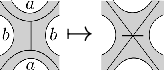
Figure 14. Constructing a marked graph in from an -system in Lemma 3.4a. Conversely, given a marked graph , the inverse of the operation in Figure 14, creates an -system. The move on marked graphs in corresponds to the slide move in Figure 15 on -systems.

Figure 15. The slide move for -systems in in Lemma 3.4a. One can use slide moves to bring any -system into a form where there exist two open intervals with such that of the paths have one endpoint in and one endpoint on for and the remaining paths have both endpoints adjacent to each other in . The claim that any two such -systems are related by slide moves can be deduced from Kamada [Kam, Proposition 2.14].
Note that the set of -systems up to the action of is infinite, if has four or more boundary components. However in this case may still be finite if admits many symmetries in , say if (in which case all of the -systems convert into one of finitely many marked graphs up to the action of ).
- b)
If is related to by an or move then and are related by and moves. If and are related by an move then and and are related by moves. If and are related by an move then and are related by and moves.
- c)
We consider each -move separately. Assume an move takes to and creates an -labelled boundary component. Then one may obtain an -system for from any -system for by connecting an extra path to the new simple closed curve parallel to the new -labelled boundary component. This corresponds to an move. Thus and are related by and moves. If the move involves a -labelled boundary component the same reasoning may be used except with the dual notion of -systems, and and will be related by and moves.
Assume now and are related by an move. Any move determines two disjoint simple paths with and . If either path cobounds with a segment of an embedded disk in , then the move can be realized as an equivalence of -surfaces in . Thus assume neither path cobounds such a disk. First consider the case where are in different components of . One can find an -system in the component containing such that is one of the paths of the -system and similarly one can find a -system in the component containing such that is one of the paths of the -system. By finding or -systems in the remaining components of , we obtain a marked graph for which the move corresponds to an move taking to some . Thus and are related by and moves. Now consider the case where are in the same component of . Since we assumed neither cobounds with an embedded disk in , the componet of containing must have at least two -labelled and two -labelled boundary components. We must find an -system for this component of , such that is one of the paths of the -system and is one of the paths of the dual -system (any -system induces a unique dual -system and vice versa). This amounts to finding an -system for which is one of the paths of the -system and transversely intersects some other path in this -system (not ) exactly once. It is not difficult to see that any such path along with , can be extended to an -system so we are done. As before, we obtain a marked graph for which the move corresponds to an move taking to some . Thus and are related by and moves.
Assume finally that and are related by an move. The move determines a simple compact interval in with one endpoint in and the other in . We can readily find an -system in for which all paths in the system are disjoint from . This -system gives rise to a marked graph for which . Thus and are related to by moves and hence are related to each other by moves.
- d)
For the move this should be clear. For the and moves, the isotopies in connecting and are given in Figures 16 and 17.

Figure 16. An isotopy between and when and are related by an move. 
Figure 17. An isotopy between and when and are related by an move.
∎
Remark 3.5.
Lemma 3.4 might generalize to -surfaces in , without restricting to in some instances as we have done.
4. A map from broken surface diagrams to -surfaces
In Definition 4.1 we describe the function , assigning to any branch-free broken surface diagram an -surface. In Lemma 4.3 we prove some properties of the function and observe how it behaves when , , , , and moves are performed on the input. In Theorem 4.4 we prove the main result, that two marked graphs representing isotopic -links are related by a sequence of Yoshikawa moves.

Definition 4.1.
We define the function by the transformations in Figure 18, with a caveat. If the surface obtained via Figure 18 has no -labelled (resp. -labelled) boundary components, we add arbitrarily a small -labelled (resp. -labelled) boundary component to fulfil the second property of Definition 3.2. However we will often not bother to draw these extra components.

Remark 4.2.
If is such that , the set is an embedded -regular graph, possibly with some components having no vertices. Each edge or closed component gives rise to one -labelled boundary component in . The surface is indeed an -surface. The -labelled boundary forms an unlink and the existence of a -labelled boundary component at each edge forces to form an unlink as well. The isotopy class agrees with the isotopy class of . Note also that the -surface for any induces the -framing on each of its boundary components.
Lemma 4.3.
- a)
If and there exist systems and of disks in such that:
- -
and ,
- -
each disk is embedded and is of one of the types in Figure 19, based on its intersections with other disks and (which is not depicted in the figure),
then is related by -moves to a surface of the form for some .
- -
- b)
If then is related by -moves to an -surface of the form for some .
- c)
If two broken surface diagrams are related by an , , , , or move then and are related by -moves.
Proof.
- a)
Each boundary component of the -surface is an unknot and has an induced framing from the embedding . Due to the way intersects the described systems of disks, it must be the case that induces the -framing on each of its boundary components. The union is a generic projection with no branch points. The surface is nearly in the form , we must only eliminate all boundary components bounding disks of type , or . If there are disks of type or , then those boundary components of should be eliminated with moves. If there are disks of type then those boundary components may be eliminated with and moves. Once this has been done, we have .
- b)
First we show that we can use moves to ensure each boundary component of is -framed. It is enough to prove this when is connected. By the second property of Definition 3.2, has at least one -labelled and one -labelled boundary component. We can use moves to ensure that all framings are except for one -labelled boundary component. By Lemma 3.4a there is with and . The graph is planar, and we can unknot it to some plane graph in , while preserving the framings. In this form it is easy to see that this final -labelled boundary component must automatically be -framed, thus it must be -framed in as well.
Let and be systems of disks as in the definition of the function, for the surface . Let and . Note that is a disjoint union of embedded disks in , as is . Since each component of is -framed, we may assume that and are contained in the interiors of and . We perturb and so that , and are transverse in . We also assume that is transverse in , etc. Now with such a system of disks, is a generic projection of with no branch points. Ultimately, we would like to find systems of disks as in Lemma 4.3a.

Figure 20. Three desirable possibilities for a component of intersecting in Lemma 4.3a. Our next goal is to make a series of adjustments to , so that each component of intersects in one of the three ways in Figure 20. We may use moves to add extra -labelled boundary components so that contains no closed curves. Specifically, for each closed curve in this intersection we create a -labelled boundary component in a neighbourhood of some point on the curve. The closed curve then is replaced with a compact interval, as for example in the first row of Figure 21. We may use moves to add extra -labelled boundary components, followed by moves so that each disk in intersects in exactly one compact interval, as in the second row of Figure 21. We make further adjustments by shrinking each boundary component in small enough (via an equivalence in of the surface ), so that each component of intersects as in the top-left of Figure 22, possibly with more transverse intersections from (the figure depicts two such intersections). We then may use a series of and moves as in Figure 22, to achieve our stated goal of having each component of intersect in one of the three ways in Figure 20.

Figure 21. Adjusting in the proof of Lemma 4.3a. 
Figure 22. Further adjustments of in Lemma 4.3a, so that each component of intersects in one of the three ways in Figure 20. The union remains a generic projection with no branch points, and the disk systems and remain embedded in . Each triple point of arises from a component of as in the top-left of Figure 20. We perform moves to add an -labelled boundary component at each triple point, as in Figure 23. By now, for each we have that is a disjoint union of simple closed curves and compact intervals with endpoints in . Each compact interval in is properly contained in an edge of and each simple closed curve in is disjoint from any triple point in and remains a split simple closed curve in . We repeat the steps of Figure 21 for the disks with the roles of and reversed. At this point, the systems and of disks satisfy the conditions of Lemma 4.3a and we are done.

Figure 23. Adding an -labelled boundary component at a triple point. - c)
We must check that each of the mentioned moves on branch-free broken surface diagrams can be realized by -moves on their images under the function. See Figures 24, 25, 27 and 29 for the , , and moves. The reader should verify that the transitions in each figure are achievable by -moves and equivalences in . For the move, Figure 26 shows the necessary changes to the bottommost sheet, which will have only -labelled boundary components. One may use and moves to merge all -labelled boundary components into a single boundary component, the sheet can then be pushed via an equivalence in past the triple point (or where it normally would be), and then the -labelled boundary components can be restored with and moves. In the figure, the dashed line indicates where the other three sheets would intersect the bottommost sheet in the broken surface diagram.
Instead of the move, in Figure 28 we check a move that is equivalent to modulo , , , and moves.
∎


Theorem 4.4.
If are such that and are isotopic -links, then and are related by a sequence of Yoshikawa moves.
Proof.
Let and . By Lemma 4.3b there exists an -surface related by -moves to so that is of the form for some for . Since represents a -link isotopic to the -link represented by , by Roseman’s theorem there is a sequence of Roseman moves from to . By Theorem 2.9 there is a sequence of , , , , and moves taking to . By Lemma 4.3c there is a sequence of -moves taking to . Thus there is a sequence of -moves taking to . By Lemma 3.4c there is a sequence of Yoshikawa moves taking to .
Note also that if we are presented with marked graph diagrams of and , then the marked graph diagrams are related by a sequence of and Yoshikawa moves, by the above and the results of Kauffman [Kau] for diagrams of -regular rigid vertex spatial graphs. ∎
References
- [BKF] D. Bar-Natan, J. Fulman, L. H. Kauffman, An elementary proof that all spanning surfaces of a link are tube-equivalent, J. Knot Theory Ramifications, Vol. 7, Iss. 7 (1998), 873–879.
- [CKS] J. S. Carter, S. Kamada, and M. Saito, Surfaces in 4-space, Encyclopaedia of Mathematical Sciences: Low Dimensional Topology III, Vol. 142, Springer, (Berlin, 2004).
- [CS] J. S. Carter and M. Saito, Canceling branch points on projections of surfaces in 4-space, Proc. Amer. Math. Soc., Vol. 116, No. 1, (1992), 229–237.
- [Kam] S. Kamada, Braid and Knot Theory in Dimension Four, Mathematical Surveys and Monographs, Volume 95, American Mathematical Society, (2002).
- [Kau] L. H. Kauffman, Invariants of Graphs in Three-Space, Transactions of the American Mathematical Society, Vol. 311, No. 2, (1989), 697–710.
- [KK] C. Kearton, V. Kurlin, All -dimensional links in -space live inside a universal -dimensional polyhedron, Algebraic & Geometric Topology 8 (2008), 1223–1247.
- [L] S. J. Lomonaco, Jr., The homotopy groups of knots I. How to compute the algebraic 2-type, Pacific J. Math., Vol. 95, No. 2, (1981), 349–390.
- [R] D. Roseman, Reidemeister-type moves for surfaces in four-dimensional space, Knot Theory, Banach Center Publications, Vol. 42, Institute of Mathematics, Polish Academy of Sciences, Warszawa, (1998), 347–380.
- [S] F. Swenton, On a calculus for -knots and surfaces in -space, J. Knot Theory Ramifications, Vol. 10, Iss. 08, (2001).
- [TT] M. Takase and K. Tanaka, Regular-equivalence of -knot diagrams and sphere eversions, Mathematical Proceedings of the Cambridge Philosophical Society, Volume 161, Issue 2, September 2016, 237–246.
- [Yo] K. Yoshikawa, An enumeration of surfaces in four-space, Osaka J. Math. 31 (1994), 497–522.