Modelling the Milky Way’s globular cluster system

Piffl et al. (2014) sought an axisymmetric Galactic potential that is consistent with a wide range of observational data. Specifically, they required the potential to reproduce gas terminal velocities at various longitudes, the kinematics of stellar masers with very precise astrometry, the proper motion of Sgr A*, the run of stellar density with distance from the Galactic plane near the Sun, and the kinematics of $\sim 200\,000$ stars in the RAdial Velocity Experiment (Steinmetz et al., 2006; Kordopatis et al., 2013, RAVE;). The potential assumes that the Galaxy’s mass is dominated by a gas disc, thin and thick stellar discs, a stellar bulge and a dark halo. The disc components are described by density distributions of the form

where $(R,z)$ are cylindrical coordinates in the Galactocentric frame, $R_{\mathrm{d}}$ and $z_{\mathrm{d}}$ are characteristic scales, and $\Sigma_{0}$ is the surface density of the disc. A non-zero value of $R_{\textup{hole}}$ allows for a central cavity.

The stellar bulge and dark halo have

where

Here, $\rho_{0}$ is a normalisation constant, $r_{0}$ is a scale radius, and $q$ is the axis ratio for surfaces of constant density. The exponential term permits the spheroids to extend only to a finite distance set by $r_{\textup{cut}}$, and also ensures that the density profile has a finite mass for all sensible values of $a$ and $b$. The Galactic potential $\Phi(R,z)$ is then given by solving the Newton–Poisson equation.

As the constraints adopted by Piffl et al. (2014) are probes of the vertical profile of gravitating matter, both baryonic and dark, their data are consistent with a model with a spherical dark halo and a heavier baryonic disc, or a more flattened dark halo and a lighter baryonic disc. Consequently, the axis ratio $q\leq 1$ of the dark halo is not tightly constrained, although Piffl et al. (2014) argue that a comparison with the results of Bienaymé et al. (2014) favours an axis ratio $q\simeq 0.8$. We have chosen to use $q=0.8$ for the dark halo, although a larger value has no significant effect on our results. The full set of parameter values we used for the gravitational potential are shown in Table 1. Section 2.3 of Binney & McMillan (2016) gives details of downloadable code that evaluates $\Phi(R,z)$ and its derivatives given the numbers in Table 1.

Note that the GC system does not enter into this model because its mass is negligible. We treat the GCs as a system of 157 identical, non-interacting point particles moving in the static potential $\Phi(R,z)$, each with Hamiltonian

The velocity components $v_{R}$ and $v_{z}$ are in the radial and vertical directions respectively, and $J_{\phi}\equiv Rv_{\phi}$ is the conserved angular momentum about the axis of Galactic rotation. Positive velocity $v_{\phi}$ is in the direction of Galactic rotation.

We define the set of observables for a GC as

where $(l,b)$ are the Galactic longitude and latitude, $s$ is the heliocentric distance, $v_{\mathrm{los}}$ is the line-of-sight velocity, and $\bm{\mu}\equiv(\mu_{\alpha}^{*}=\dot{l}\cos b,\mu_{\delta}=\dot{b})$ is the proper motion vector.

In order to transform these into the phase space coordinates

we have assumed that the Sun is located at $(R,\phi,z)=(R_{0},0,0)$, where we take $R_{0}=8.3\,\mathrm{kpc}$ (Schönrich, 2012). We further assume that the local circular speed is $240\,\mathrm{km}\,\mathrm{s}^{-1}$ (Schönrich, 2012), and that the Sun has velocity $\bm{(}U,V,W)_{\odot}=(11.1,12.24,7.25)\,\mathrm{km}\,\mathrm{s}^{-1}$ (Schönrich, Binney & Dehnen, 2010) relative to the local standard of rest (LSR). Positive velocities $U$, $V$ and $W$ point in the direction of the Galactic centre, Galactic rotation and Galactic north pole respectively.

It proves useful to transform these phase space coordinates into angle–action variables $(\bm{\theta},\bm{J})$. These are a set of canonical coordinates where the momenta $J_{i}$ are integrals of motion. It then follows from Hamilton’s equations that $H\equiv H(\bm{J})$ and the angles $\theta_{i}$ increase linearly with time (Binney & Tremaine, 2008). The orbit of a GC is specified by $\bm{J}$, and if at time $t=0$ it is at position $\bm{x}(\bm{\theta}(0),\bm{J})$, then we simply increase the angles linearly to evolve the position forwards in time. Despite its advantages, this formalism has until recently been little used on account of the difficulty in evaluating $(\bm{\theta},\bm{J})$. Recent technical progress now makes this possible. We make extensive use of the Stäckel Fudge (Binney, 2012; Sanders & Binney, 2016), which yields $(\bm{\theta},\bm{J})$ given $(\bm{x},\bm{v})$ in an axisymmetric potential like that of Section 2.1. We identify $\bm{J}\equiv(J_{r},J_{z},J_{\phi})$, where $J_{r},J_{z}\geq 0$ can be thought of as quantifying oscillations in the radial and vertical directions.

Given that the GC system is in dynamical equilibrium, Jeans’ (1915) theorem allows us to assume that the DF is a function $f(\bm{J})$, so the probability that a randomly chosen GC has phase-space coordinates in $\mathrm{d}^{3}\bm{\theta}\,\mathrm{d}^{3}\bm{J}$ is

We normalize $f(\bm{J})$ such that

so the quantity $(2\pi)^{3}f(\bm{J})\;\mathrm{d}^{3}\bm{J}$ gives the probability that a randomly selected GC moves on the orbit specified by $\bm{J}$.

Although we do not assume that the metal-rich clusters form a disc-like component and the metal-poor clusters form a spheroid, our DF is a linear combination of a DF for a disc-like population and a DF for a halo population. We write

where $F_{\textup{disc}}\in[0,1]$ is the fraction of disc GCs and $\Pi$ is a set of parameters for the model. We will often write $f(\bm{J}|\Pi)$ as simply $f(\bm{J})$ in what follows, but they will mean the same thing. It turns out that favoured models assign roughly as much probability to the disc-like component as the fraction of observed clusters that are metal rich, but this is an empirical result rather than an assumption.

The DF of an axisymmetric system is usually best considered to be the sum of a part $f_{+}$ even in $J_{\phi}$ and a part $f_{-}$ odd in $J_{\phi}$. The latter does not contribute to the density of the system, but is largely responsible for the system’s rotation. If we wish to avoid discontinuities in the DF, $f_{-}$ must vanish with $J_{\phi}$. A convenient way to satisfy this condition and obtain a non-negative and physically reasonable DF is to posit

Here $-1\leq k\leq 1$ is a constant that controls the sign and intensity of any rotation, and $L$ is a constant that controls the steepness of the system’s central rotation curve. We have used this ansatz for the odd parts of the DFs of both disc and halo.

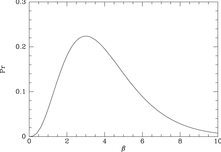
As we are interested in how the GC data constrain the parameters of this model, we opt for the least informative prior possible. The variables $k_{\textup{d}},k_{\textup{h}}\in[-1,1]$ and $F_{\textup{disc}}\in[0,1]$ have finite ranges, so we take the prior to be uniform in these ranges. The scale parameters $L_{\textup{d}}$, $L_{\textup{h}}$, $J_{0}$, $\sigma_{i0}$, and $\mathcal{R}_{\textup{d}}$ are intrinsically positive, so the unbiased prior is uniform in the logarithms of these quantities (Jeffreys, 1961). The indices $\alpha,\beta$ can, in principle take arbitrarily large positive values, but if we require only $\beta>0$, the data yield a degeneracy in which both $\beta$ and $J_{0}$ increase. From the work of Posti et al. (2015) and Das & Binney (2016) we expect $\beta\sim 5$. To incorporate this knowledge into our prior, we take the prior on $\beta$ to be the gamma distribution

where $A$ and $B$ are hyperparameters and $\Gamma(A)$ is the gamma function. We set $A=4$ and $B=1$ such that the distribution has a mean $\beta=4$, a mode $\beta=3$, and a variance of $4$. With this prior on $\beta$, implausibly large values of $\beta$ and $J_{0}$ acquire low values of the posteriori probability, but it might be argued that a weaker prior would be preferable. We have investigated two priors on the inverse distance $\gamma$: uniform and uniform in its logarithm.

In summary, our prior is

where, as discussed in Section 4 $\textup{Pr}(\gamma)$ is successively (i) uniform in $\gamma$, (ii) uniform in $\log\gamma$, and (iii) $\delta(\gamma)$.

Data on the position variables $(l,b,s)$ of the 157 known GCs were obtained from the 2010 edition of the Harris 1996 catalogue. This catalogue also contains line-of-sight velocities for 143 of these GCs. Proper motion data exist for only 64 GCs; these have been obtained from Massari et al. (2013) and a catalogue by Casetti–Dinescu et al. (2013)²² 2 The proper motions catalogue can be accessed at http://www.astro.yale.edu/dana/gc.html..

The Galactic coordinates $(l,b)$ are measured to high precision, so the effects of their errors will be neglected. The errors in the remaining observable quantities are assumed to be independent. If $u\in\{v_{\mathrm{los}},\mu^{*}_{\alpha},\mu_{\delta}\}$ denotes a component of velocity, then we assume that its measured value $\bar{u}$ is related to its true value $u$ by the Gaussian distribution

where $\sigma_{u}$ is the uncertainty in $u$. Where possible, the values of $\bar{u}$ and $\sigma_{u}$ are obtained from the data sources listed above. When no such data are available, following MB13 the value of $\sigma_{u}$ is taken to be sufficiently large that the Gaussian distribution is effectively constant for all sensible values of $u$.

Since heliocentric distance $s$ is an intrinsically positive quantity, we take its probability distribution to be a lognormal distribution

where following (Casetti–Dinescu et al., 2013) the values of $\sigma_{s}$ and $\mathcal{S}(\bar{s},\sigma_{s})$ are chosen such that the distribution has a mean equal to the measured distance $\bar{s}$ and a variance of $(0.1\bar{s})^{2}$. Actually the uncertainties in cluster distances are surely sometimes smaller and sometimes larger than this estimate, so this work could be upgraded by obtaining errors on individual cluster distances. We shall see also that it would be very desirable to take pains to ensure that all cluster distances are assigned using the same value of $R_{0}$ as that adopted for the model.

For brevity, we use the notation

to describe the six-dimensional error distribution for the observables of the $\eta^{\textup{th}}$ GC.

While MB13 include the apparent magnitude $m$ as an observable, we do not because we assume the completeness of our sample is independent of magnitude. The likelihood $\mathcal{L}$ that the GC data are drawn from the model $f(\bm{J})$ is the product

where $\mathrm{Pr}(\bm{u}|\textup{Model})$ is the probability that a randomly chosen GC has true observables $\bm{u}$:

with

Here the coordinates $(\bm{\theta},\bm{J})$ are evaluated at the given point $\bm{u}$, and the selection function $S(\bm{u})$ gives the probability that if a GC with true observables $\bm{u}$ exists, it has been included in the Harris and Casetti–Dinescu catalogues. The normalisation constant $A$ is given by the condition $\int{\rm d}^{6}{\bm{u}}\,\mathrm{Pr}(\bm{u}|\textup{Model})=1$, so

We MCMC sample the posterior distribution as follows:

1. 1.

   Sample $N_{\textup{S}}$ points from $f_{\textup{S}}(\bm{x},\bm{v})$ and $N_{\eta}$ points for each GC from $\xi(\bm{u}|\bm{u}^{\eta})$. These are independent of $f(\bm{J})$ so need only be sampled once at the beginning.

2. 2.

   Use the Schlegel et al. (1998) map to determine the selection function $S(\bm{u})$ for each of the above $N_{\textup{S}}$ points.

3. 3.

   Use the Stäckel fudge (Binney, 2012; Binney, 2014) with the gravitational potential $\Phi$ in Section 2.1 to calculate $\bm{J}$ for each of these points.

4. 4.

   Pick a point $\Pi$ in the space of model parameters at random.

5. 5.

   Calculate the prior $\textup{Pr}(\Pi)$ using equations (17) and (18).

6. 6.

   If $\textup{Pr}(\Pi)\neq 0$, calculate the likelihood $\mathcal{L}$ for the model $f(\bm{J}|\Pi)$ using equations (27) and (28).

7. 7.

   Calculate the posterior $\textup{Pr}(\Pi|\textup{Data})$ using equation (16).

8. 8.

   We use a robust adaptive Metropolis algorithm (Vihola, 2012) to decide on the next point $\Pi$ in the Markov chain.

9. 9.

   Repeat steps 5 to 8 until the desired number of MCMC points have been sampled.

We have sampled $50\,000$ MCMC points, and we have used $N_{\eta}=100$ and $N_{\textup{S}}=157\times N_{\eta}$, the latter choice made such that an equal number of points are evaluated for the numerator and denominator of $\mathcal{L}$.

We can probe the impact of noise, and the extent to which a model can match the data by using a model to generate pseudo-catalogues of clusters. We generate a pseudo-catalogue as follows:

1. 1.

   Sample a phase-space point $(\bm{x},\bm{v})$ for a ‘pseudo-GC’ from $f(\bm{J}(\bm{x},\bm{v})|\Pi)$ and compute the observables $\bm{u}$.

2. 2.

   Accept the pseudo-GC with probability given by the selection function $S(\bm{u})$ and return to the previous step until 157 pseudo-GCs have been accepted.

3. 3.

   The observables of each pseudo-GC are ascribed errors $\bm{\sigma}$ according to the error model described below.

4. 4.

   The observables $\bm{u}$ are scattered by their errors.

The line-of-sight velocities $v_{\mathrm{los}}$ have errors that approximately follow a lognormal distribution (see Fig. 2). A priori, we might expect that these errors depend on the heliocentric distance $s$, but by plotting errors in $v_{\mathrm{los}}$ versus distance $s$ in the Harris catalogue, the lower plot of Fig. 2 demonstrates that errors in $v_{\mathrm{los}}$ do not increase significantly with $s$. Consequently, each GC in a pseudo-catalogue is given an error randomly drawn from the same lognormal distribution.

As more than half of the GCs do not have proper motion data, quantities calculated using the proper motions will come with very large uncertainties, and we do not consider these useful to decide if a model agrees with data. We therefore have not concerned ourselves with modelling the error distribution of the proper motions, and will restrict ourselves to analysing pseudo-catalogues using only the observables $(l,b,s,v_{\mathrm{los}})$.

Equation (10) applied to the halo and disc DFs defines four parameters $k_{\textup{h}}$, $L_{\textup{h}}$, $k_{\textup{d}}$ and $L_{\textup{d}}$ that control the amplitude and central steepness of each system’s rotation curve. Along early MCMC chains the posterior distributions of $L_{\textup{h}}$ and $L_{\textup{d}}$ were indistinguishable from their priors (uniform in $\log L_{i}$). Moreover, no correlation was apparent between $L_{i}$ and any other parameter of the DF. Evidently, the data do not usefully constrain the steepness of the central rotation curves of the components, so in the following we simply adopt $L_{i}=100\,\mathrm{kpc}\,\mathrm{km}\,\mathrm{s}^{-1}$, which we shall find causes the rotation curves of the disc and halo populations to have central slopes $\sim 100\,\mathrm{km}\,\mathrm{s}^{-1}\,\mathrm{kpc}^{-1}$.

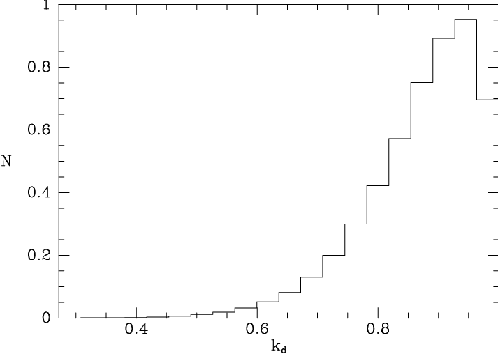
Fig. 3 shows the posterior distribution of $k_{\textup{d}}$, which is crowded near the upper limit of its permitted range. The crowding of the posterior distribution of $k_{\textup{d}}$ near unity implies a lack of evidence for a counter-rotating disc of clusters. Consequently, in the following we set $k_{\textup{d}}=1$.

In early MCMC exploration of parameter space we adopted a uniform prior on the parameter $\gamma$ that controls the radial variation of the disc’s velocity dispersions (eqn. 13). The posterior distribution of $\gamma$ then extended both sides of zero. Since we consider increases in velocity dispersion with radius implausible, we then ran chains with the prior on $\gamma$ taken to be uniform in $\log\gamma$. The resulting posterior distribution of $\gamma$ was essentially uniform in $\log\gamma$ for $\gamma<10^{-6}\,\mathrm{kpc}^{-1}$. That is, the data only require that $\gamma$ is so small as to have negligible impact in the region $r<100\,\mathrm{kpc}$ to which the data are confined. This being so, we subsequently set $\gamma=0$, i.e., we made the velocity-dispersion parameters independent of $J_{\phi}$.

In summary, we fix the values of four parameters:

leaving the posterior distributions of eight parameters to be explored by MCMC chains. Of these four describe the halo DF ($\alpha$, $\beta$, $k_{\textup{h}}$ and $J_{0}$), three describe the disc DF ($\mathcal{R}_{\textup{d}}$, $\sigma_{r}$ and $\sigma_{z}$), and the eighth and final adjustable parameter is $F_{\textup{disc}}$, which is the fraction of the probability associated with the disc.

Fig. 4 illustrates the structure of the posterior distributions of all adjustable parameters by showing on the diagonal histograms for each parameter after marginalising over all other parameters, and in the off-diagonal panels the correlations between each pair of model parameters, again after marginalising over all other parameters. The white contours in the off-diagonal panels enclose 68 per cent of the probability.

Parameters that are quite well determined are the extent to which the halo cluster distribution rotates $k_{\rm h}$, the fraction of disc clusters $F_{\textup{disc}}$, the velocity-dispersion parameters of the disc clusters $\sigma_{r}$ and $\sigma_{z}$, and the scale length of the system of disc clusters $\mathcal{R}_{\textup{d}}$. For each parameter, Table 2 gives the expectation value and the standard deviation along the MCMC chain.

Three parameters for the halo clusters are strongly correlated: the inner and outer slope parameters $\alpha,\beta$ and the scale action $J_{0}$. Large values of $J_{0}$ are associated with large values of $\alpha$ and $\beta$. This correlation makes perfect sense physically when one recalls that $\alpha$ and $\beta$ control the inner and outer slopes of the real-space density profile of the population of halo clusters, while $J_{0}$ controls the break radius that divides the two regimes. In so far as the density profile of the halo cluster distribution steepens smoothly with increasing radius, such a correlation between $\alpha$, $\beta$ and $J_{0}$ and is inevitable. Naively, one expects $J_{0}$ to be roughly the product of the circular speed and the radius $\sim 2.5\,\mathrm{kpc}$ of the break in the density profile, so $\sim 600\,\mathrm{kpc}\,\mathrm{km}\,\mathrm{s}^{-1}$. The probable values of $J_{0}$ are significantly larger than this. However, we show below that the recovered parameter values do reproduce the expected break radius.

Fig. 5 shows the distribution of the likelihoods of the data given the models sampled by MCMC. This distribution – essentially the $\chi^{2}$ distribution of the models – is more than two orders of magnitude wide, so significant probability is associated with models that make the data hundreds of times less probable than does the most probable model. This state of affairs is commonplace when models with significant numbers of parameters are employed in Bayesian inference.

Why must we consider models that make the data so much less probable than the maximum-likelihood model? Because the maximum-likelihood model achieves its high likelihood in large measure by fitting not only the signal but also the the noise in the data. In Fig. 6 we demonstrate this by comparing the observables predicted by samples of 157 clusters drawn from (a) the maximum-likelihood model (top row) with (b) models drawn at random from the MCMC chain (lower row). We see that the scatter around the real observables (red curves) of the observables predicted by the maximum-likelihood model and the models drawn at random are indeed similar. This result confirms that the excess likelihood of the maximum likelihood model over typical models in the MCMC chain indeed reflects its ability to fit the high level of noise inherent in there being only 157 clusters.

In Fig. 6 the only panels in which the red line of the data lies outside the region explored by the 20 realisations are those for the distance, $s$: in these panels the full red line for the data rises steeply with increasing $s$ at values of $s$ that are $\sim 10$ per cent smaller than the broken curves of the pseudo-data. The number of clusters increases rapidly as $s$ becomes comparable to $R_{0}$ and the clusters gathered around the Galactic Centre enter the sample.

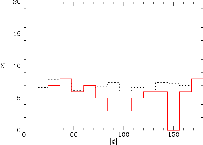
The red histogram in Fig. 7 shows the distribution of the Galactocentric azimuths of the real clusters: there is a clear excess of clusters with $|\phi|<20$ degrees, indicating that they lie in front of the Galactic Centre. By contrast, the black dashed histogram, which shows the azimuthal distribution of the clusters in twenty models from the MCMC chain, is very uniform, so we have not succeeded in modelling the distribution of clusters in the central region. The cause of this discrepancy could be either (a) that distances to clusters are systematically too short, or (b) that our value $R_{0}=8.3\,\mathrm{kpc}$ is too long, or (c) that observers have failed to identify significant numbers of clusters that lie in or behind the bulge. The latter could be due either to more extinction than we have adopted, or confusion in crowded fields. However, following the Vista Variables in the Via Lactea (VVV) survey (Minniti et al., 2010) of the bulge region in the near IR and with excellent spatial resolution, it seems unlikely that item (c) is a significant problem.

Apart from this question surrounding the distribution of cluster in the bulge region, we consider that the plots of Fig. 6 are consistent with the actual clusters being drawn from a model in the MCMC chain.

An MCMC chain encodes the probability density of each part of model space, and the DF quantifies the probability density of GCs in phase space for a given model. Consequently, if we average $f({\bm{x}},{\bm{v}})$ over models in an MCMC chain, we obtain our best estimate of the probability of finding a GC at $({\bm{x}},{\bm{v}})$. We now present plots obtained by averaging $f$ over 50 models drawn from an MCMC chain.

Fig. 8 shows the probability density of disc and halo clusters in action space. Specifically, the logarithm to base 10 of the density is shown on three slices at constant radial action, from $J_{r}=0$ (circular orbits) at the top to larger values of $J_{r}$ lower down. The two types of cluster are seen to have very different phase-space distributions. The disc clusters are most dense along the $J_{\phi}$ axis and their density declines steeply with increasing $J_{r}$ or $J_{z}$, whereas the halo clusters are dense only at the origin of action space but their density declines relatively slowly with increasing $|{\bf J}|$.

The model provides probabilities for a cluster to be a disc rather than a halo cluster based solely on the cluster’s phase-space position. It is natural to ask how these probabilities relate to the cluster’s metallicities: the latter have a clearly bimodal distribution with a minimum at $\hbox{[Fe/H]}\simeq-0.8$ (Zinn, 1985; Harris et al., 2016) dividing the metal-poor halo cluster from the metal-rich disc clusters.

Fig. 9 shows for each cluster in the Harris catalogue the ratio $\langle P_{\rm disc}\rangle/\langle P_{\rm halo}\rangle$ versus [Fe/H], where, for example $P_{\rm disc}$ is the integral in one model of the disc DF over the cluster’s error ellipsoid (eqn 22). For 73 clusters this ratio exceeds unity, so they are deemed more likely to be disc than halo clusters. Clusters with $\hbox{[Fe/H]}\ga-1.3$ are never considered much more likely to be halo clusters than disc cluster, while only a few clusters with $\hbox{[Fe/H]}<-2$ are much more likely to be disc than halo clusters. The only clusters that will be considered much more likely to be halo than disc clusters are those that counter-rotate or lie at very large radii. Inevitably, at least as many halo clusters at moderate $r$ co- rather than counter-rotate, and these clusters will have significant probabilities to be disc clusters. Hence it is to be expected that more clusters have high probabilities to belong to the disc than have $\hbox{[Fe/H]}>-0.8$. Hence Fig. 9 is fully consistent with the conjecture that all metal-rich clusters belong to the disc population, while the metal-poor clusters all belong to the halo population.

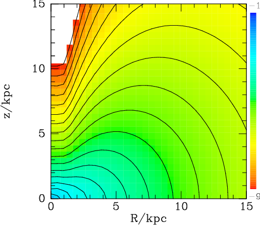
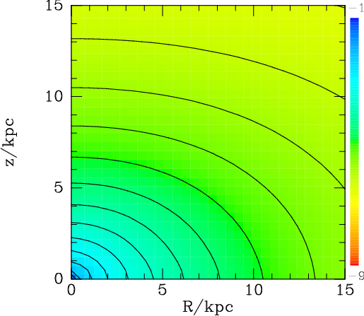
Fig. 10 shows the real-space density of disc clusters (left) and halo clusters (right) estimated from 50 models drawn at random from the MCMC chain. The colour scale shows the logarithm of the density in a slice that includes the $z$ axis. For semi-major axes of length $a\la 5\,\mathrm{kpc}$, the system of disc clusters has the isodensity contours of an oblate body with axis ratio $\sim 1:3$. Larger isodensity surfaces have a deep depression around the minor axis. Any system in which all particles rotate in the same sense about the $z$ axis can be expected to have a low density on that axis. The right panel of Fig. 10 indicates that the system of halo clusters forms a simpler oblate structure of axis ratio $q\sim 0.7$ out to semi-major axes $a\sim 20\,\mathrm{kpc}$, but a similar plot on a bigger scale shows that around $r\sim 30\,\mathrm{kpc}$ the system becomes quite spherical because the potential is then dominated by the spherical dark halo rather than the disc.

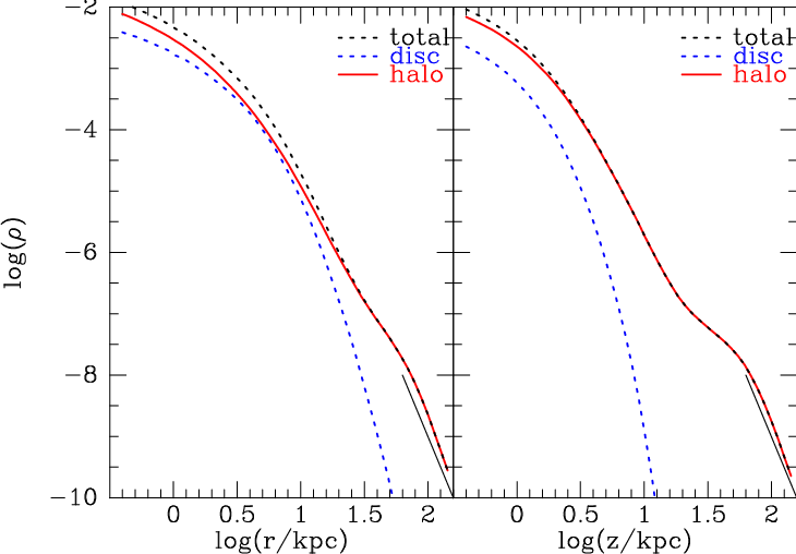
Fig. 11 shows the density of clusters as a function of radius in the equatorial plane (left panel) and along the $z$ axis (right panel). In each panel we show the contributions of the disc and halo clusters (blue and red lines, respectively) and the total density in black. Straight black lines at the lower right of each panel have slope $-5$, revealing that at the largest radii the cluster density is declining somewhat faster than as $r^{-5}$. From results in Posti et al. (2015) it is easy to show that if the rotation curve were flat, $\rho\sim r^{-5}$ would imply $f\sim|{\bm{J}}|^{-5}$. Table 2 indicates a markedly steeper decline in the DF, $f\sim|{\bm{J}}|^{-9}$, because the MCMC chain favours large values of the scale action $J_{0}$, so the asymptotic regime has not been reached even at $r\sim 80\,\mathrm{kpc}$.

The profiles of the system of halo clusters show wiggles at $R,z\ga 20\,\mathrm{kpc}$. The wiggle on the $z$ axis is most pronounced. This feature disappears when the disc’s potential is removed and the dark halo’s potential is enhanced in compensation, so it arises from the response of the cluster system to the fading of the disc’s gravitational field. It coincides with the decrease in flattening noted above in connection with Fig. 10.

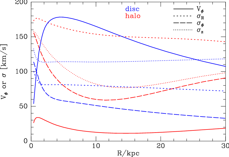
Fig. 12 shows the kinematics computed from 50 models as a function of radius in the equatorial plane. As the centre is approached, the three broken red curves, which show $\sigma_{R}$, $\sigma_{\phi}$ and $\sigma_{z}$ in the halo system, approach one another at quite a large value: $\sim 170\,\mathrm{km}\,\mathrm{s}^{-1}$. While the centre of the halo system is isotropic, with increasing $R$ the curves for $\sigma_{\phi}$ and $\sigma_{z}$ fall much more steeply than the curve for $\sigma_{R}$, so the body of the system is quite radially biased: the conventional anisotropy parameter $\beta_{\rm s}$ reaches a peak value $0.68$ at $R=12\,\mathrm{kpc}$ and then gently falls to $\beta_{\rm s}=0.53$ at $R=30\,\mathrm{kpc}$. The full red curve shows that the mean rotation rate of the halo system is small – it peaks at $\langle v_{\phi}\rangle\sim 40\,\mathrm{km}\,\mathrm{s}^{-1}$ at $R\sim 1\,\mathrm{kpc}$ and from there falls to a minimum of $12\,\mathrm{km}\,\mathrm{s}^{-1}$ around $R=15\,\mathrm{kpc}$.

The disc system rotates fast: its rotation curve reaches $\langle v_{\phi}\rangle=185\,\mathrm{km}\,\mathrm{s}^{-1}$ at $R=5\,\mathrm{km}\,\mathrm{s}^{-1}$ and from there $\langle v_{\phi}\rangle$ falls almost linearly to $118\,\mathrm{km}\,\mathrm{s}^{-1}$ at $R=30\,\mathrm{kpc}$. The velocity dispersion tensor is quite anisotropic, with $\sigma_{z}\sim 100\,\mathrm{kpc}$ being largest and $\sigma_{\phi}$ falling from $\sim 50\,\mathrm{km}\,\mathrm{s}^{-1}$ at $R=3\,\mathrm{kpc}$ to $\sim 30\,\mathrm{km}\,\mathrm{s}^{-1}$ at $R=30\,\mathrm{kpc}$.

As we reported in Section 3.3.3, the algorithm of Frenk & White (1980) applied to the complete Harris catalogue yields a rotation velocity $v_{\textup{rot}}=79\,\mathrm{km}\,\mathrm{s}^{-1}$. When we assemble a catalogue of 157 clusters from each of 20 models from the MCMC chain and apply the Frenk & White algorithm to each catalogue, the recovered values of $v_{\textup{rot}}$ have mean $69\,\mathrm{km}\,\mathrm{s}^{-1}$ and standard deviation $29\,\mathrm{km}\,\mathrm{s}^{-1}$. Thus our models are consistent with the data from the perspective of rotation rate.

References

- Bica et al. (2006) Bica E., Bonatto C., Barbuy B., Ortolani S., 2006, A&A, 450, 105
- Bienaymé et al. (2014) Bienaymé O., et al., 2014, A&A, 571, A92
- Binney (2010) Binney J., 2010, MNRAS, 401, 2318
- Binney (2012) Binney J., 2012, MNRAS, 426, 1324
- Binney (2014) Binney J., 2014, MNRAS, 440, 787
- Binney & McMillan (2011) Binney J., McMillan P., 2011, MNRAS, 413, 1889
- Binney & McMillan (2016) Binney J., McMillan P. J., 2016, MNRAS, 456, 1982
- Binney & Tremaine (2008) Binney J., Tremaine S., 2008, Galactic Dynamics: Second Edition. Princeton University Press
- Bovy et al. (2016) Bovy J., Rix H.-W., Schlafly E. F., Nidever D. L., Holtzman J. A., Shetrone M., Beers T. C., 2016, ApJ, 823, 30
- Casagrande et al. (2011) Casagrande L., Schönrich R., Asplund M., Cassisi S., Ramírez I., Meléndez J., Bensby T., Feltzing S., 2011, A&A, 530, A138
- Casetti–Dinescu et al. (2013) Casetti–Dinescu D. I., Girard T. M., Jílková L., van Altena W. F., Podestá F., López C. E., 2013, AJ, 146, 33
- Das & Binney (2016) Das P., Binney J., 2016, MNRAS, 460, 1725
- Das et al. (2016) Das P., Williams A., Binney J., 2016, MNRAS, 463, 3169
- Frenk & White (1980) Frenk C. S., White S. D. M., 1980, MNRAS, 193, 295
- Gnedin et al. (2014) Gnedin O. Y., Ostriker J. P., Tremaine S., 2014, ApJ, 785, 71
- Harris (1996) Harris W. E., 1996, AJ, 112, 1487
- Harris (2001) Harris W. E., 2001, in Labhardt L., Binggeli B., eds, Saas-Fee Advanced Course 28: Star Clusters. p. 223
- Harris & Canterna (1979) Harris W. E., Canterna R., 1979, ApJ, 231, L19
- Harris et al. (2016) Harris W. E., Blakeslee J. P., Whitmore B. C., Gnedin O. Y., Geisler D., Rothberg B., 2016, ApJ, 817, 58
- Hernquist (1990) Hernquist L., 1990, ApJ, 356, 359
- Holmberg et al. (2007) Holmberg J., Nordström B., Andersen J., 2007, A&A, 475, 519
- Holmberg et al. (2009) Holmberg J., Nordström B., Andersen J., 2009, A&A, 501, 941
- Jaffe (1983) Jaffe W., 1983, MNRAS, 202, 995
- Jeans (1915) Jeans J. H., 1915, MNRAS, 76, 70
- Jeffreys (1961) Jeffreys H., 1961, Theory of Probability. Clarendon Press
- Kordopatis et al. (2013) Kordopatis G., et al., 2013, AJ, 146, 134
- Kurtev et al. (2008) Kurtev R., Ivanov V. D., Borissova J., Ortolani S., 2008, A&A, 489, 583
- Mackey & Gilmore (2004) Mackey A. D., Gilmore G. F., 2004, MNRAS, 355, 504
- Majewski et al. (2016) Majewski S. R., APOGEE Team APOGEE-2 Team 2016, Astronomische Nachrichten, 337, 863
- Massari et al. (2013) Massari D., Bellini A., Ferraro F. R., van der Marel R. P., Anderson J., Dalessandro E., Lanzoni B., 2013, ApJ, 779, 81
- McMillan & Binney (2013) McMillan P. J., Binney J. J., 2013, MNRAS, 433, 1411
- Minniti et al. (2010) Minniti D., et al., 2010, New Astron., 15, 433
- Navarro et al. (1996) Navarro J. F., Frenk C. S., White S. D. M., 1996, ApJ, 462, 563
- Piffl et al. (2014) Piffl T., et al., 2014, MNRAS, 445, 3133
- Piffl et al. (2015) Piffl T., Penoyre Z., Binney J., 2015, MNRAS, 451, 639
- Posti et al. (2015) Posti L., Binney J., Nipoti C., Ciotti L., 2015, MNRAS, 447, 3060
- Sanders & Binney (2015) Sanders J. L., Binney J., 2015, MNRAS, 449, 3479
- Sanders & Binney (2016) Sanders J. L., Binney J., 2016, MNRAS, 457, 2107
- Schlegel et al. (1998) Schlegel D. J., Finkbeiner D. P., Davis M., 1998, ApJ, 500, 525
- Schönrich (2012) Schönrich R., 2012, MNRAS, 427, 274
- Schönrich et al. (2010) Schönrich R., Binney J., Dehnen W., 2010, MNRAS, 403, 1829
- Steinmetz et al. (2006) Steinmetz M., et al., 2006, AJ, 132, 1645
- Thomas (1989) Thomas P., 1989, MNRAS, 238, 1319
- Tremaine et al. (1975) Tremaine S. D., Ostriker J. P., Spitzer Jr. L., 1975, ApJ, 196, 407
- VandenBerg et al. (2013) VandenBerg D. A., Brogaard K., Leaman R., Casagrande L., 2013, ApJ, 775, 134
- Vihola (2012) Vihola M., 2012, Statistics and Computing, 22, 997
- Williams & Evans (2015) Williams A. A., Evans N. W., 2015, MNRAS, 454, 698
- Wyse & Gilmore (1995) Wyse R. F. G., Gilmore G., 1995, AJ, 110, 2771
- Zinn (1985) Zinn R., 1985, ApJ, 293, 424
- Zinn (1993) Zinn R., 1993, in Smith G. H., Brodie J. P., eds, Astronomical Society of the Pacific Conference Series Vol. 48, The Globular Cluster-Galaxy Connection. p. 38