跳到论文正文
W Papers独立论文阅读器 arXiv:1701.06990 论文正文 计算阅读时间 · 0%
引用这篇论文根据当前论文元数据生成,正式投稿前建议核对。


License: arXiv.org perpetual non-exclusive license
arXiv:1701.06990v3 [cond-mat.mes-hall] 08 Apr 2018

Pumping of magnons in a Dzyaloshinskii-Moriya ferromagnet

Alexey A. Kovalev Affiliation: Department of Physics and Astronomy and Nebraska Center for Materials and Nanoscience, University of Nebraska, Lincoln, Nebraska 68588, USA    Vladimir A. Zyuzin Affiliation: Department of Physics and Astronomy and Nebraska Center for Materials and Nanoscience, University of Nebraska, Lincoln, Nebraska 68588, USA    Bo Li Affiliation: Department of Physics and Astronomy and Nebraska Center for Materials and Nanoscience, University of Nebraska, Lincoln, Nebraska 68588, USA
August 24, 2026
Abstract

We formulate a microscopic linear response theory of magnon pumping applicable to multiple-magnonic-band uniform ferromagnets with Dzyaloshinskii–Moriya interactions. From the linear response theory, we identify the extrinsic and intrinsic contributions where the latter is expressed via the Berry curvature of magnonic bands. We observe that in the presence of a time-dependent magnetization Dzyaloshinskii–Moriya interactions can act as fictitious electric fields acting on magnons. We study various current responses to this fictitious field and analyze the role of Berry curvature. In particular, we obtain an analog of the Hall-like response in systems with non-trivial Berry curvature of magnon bands. After identifying the magnon-mediated contribution to the equilibrium Dzyaloshinskii–Moriya interaction, we also establish the Onsager reciprocity between the magnon-mediated torques and heat pumping. We apply our theory to the magnonic heat pumping and torque responses in honeycomb and kagome lattice ferromagnets.

pacs
85.75.-d, 72.20.Pa, 75.30.Ds, 72.20.My

I Introduction

It is well known that an electric field can drive a charge current, whereas in order to understand how to drive a spin current one needs to resort to the field of spintronics [1]. Magnetization dynamics generates spin currents in adjacent normal metal by a phenomenon known as spin pumping [2; 3; 4]. The discovery of spin pumping had a great deal of influence on the development of the field of spintronics as it led to new insights into the spin Hall [5], spin torque [6; 7], and spin Seebeck effects [8]. The phenomena related to the spin Seebeck effect are studied within the field of spincaloritronics [9] in which the focus is on interplay between the spin degrees of freedom and heat currents.

As heat and spin currents are also carried by magnons, one naturally arrives at a concept of magnon-mediated spin torques which can lead to thermally induced motion of magnetic domain walls [10; 11; 12]. Such torques exist only in noncollinear magnetic structures or when the Dzyaloshinskii-Moriya interactions (DMI) are present. In the latter case, such spin torques have been termed as DMI torques [13]. Recently, both field-like and antidamping-like contributions to DMI torques have been studied theoretically [14; 15; 16; 17; 18]. It has been noted [13] that DMI torques can be seen as magnon analogs of spin-orbit torques [19; 20; 21; 22; 23; 24]. This suggests that the phenomenology developed for spin-orbit torques can be readily applied to DMI torques [25; 26]. In particular, the intrinsic contribution to DMI torques has been identified [16]. Continuing this analogy, one can identify fictitious electric fields acting on magnons due to time-dependent magnetization dynamics [27; 11; 28]. One can also identify the magnon-mediated equilibrium contribution to DMI. Due to such contribution the electron-mediated energy current calculated in response to magnetization dynamics from the Kubo formalism contains an unphysical ground-state contribution [26] which needs to be subtracted. Similar unphysical contributions have been identified for anomalous responses induced by statistical forces [29; 30; 31].

There is a considerable interest in magnets on lattices with non-trivial geometry as they allow observation of Berry phase related phenomena such as the thermal Hall effect of magnons [32; 33; 34; 35; 36; 36; 37; 38; 39; 40; 41]. Theoretically, the increased magnon damping [42], Dirac magnons [43], and the magnon-mediated spin Hall effect [16; 44; 45] have been predicted for kagome and honeycomb lattice ferromagnets. In addition, other manifestations of the Berry phase physics can arise in layered kagome [40] and honeycomb [46] ferromagnets as examined in this work.

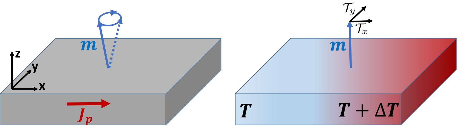
In this work, we analyze magnon currents arising in response to magnetization dynamics (see Fig. 1). In the presence of a time-dependent magnetization, DMI can act as fictitious electric fields acting on magnons. As has been noted earlier in the introduction, the energy current carried by such magnons contains the ground state contribution associated with magnon-mediated equilibrium DMI. Note that such corrections are important only in systems with non-trivial Berry curvature of magnon bands. Here, we concentrate on systems with non-trivial Berry curvature by considering various current responses in honeycomb and kagome lattice ferromagnets. Our linear response calculation of heat currents agrees with the calculation of magnon-mediated thermal torques [16], thus confirming the Onsager reciprocity principle (see Fig. 1). We also study the feasibility of experimental observation of such current responses.

The paper is organized as follows. In section II, we introduce the Hamiltonian describing magnons with multiple bands and calculate the equilibrium DMI. Next, within the same section, we describe pumping of magnons in response to magnetization dynamics and thermal torques within the linear response theory. In the final part of section II, we formulate the Onsager relations. In section III, we apply our theory to honeycomb and kagome lattice ferromagnets. We conclude our paper in section IV. The Appendices A, B, C, and D contain very detailed derivations of our results.
Refer to caption

Figure 1: (Color online) Two effects related by the Onsager reciprocity principle. Left: Magnetization dynamics pumps magnon current 𝑱p\boldsymbol{J}_{p} and spin current 𝑱s=−ℏ​𝑱p\boldsymbol{J}_{s}=-\hbar\boldsymbol{J}_{p}. This process also involves heat current 𝑱q\boldsymbol{J}_{q} carried by magnons. Right: A temperature gradient leads to a thermal torque with two components 𝒯x{\cal T}_{x} and 𝒯y{\cal T}_{y} acting on the uniform magnetization.

II Theory of magnon pumping and DMI torques

In this section, we develop a microscopic linear response theory of magnon pumping and nonequilibrium magnonic torques applicable to multiple-magnonic-band uniform ferromagnets with Dzyaloshinskii–Moriya interactions. We note that in our theory magnons are treated as conserved particles. Gilbert damping α\alpha could broaden magnonic bands and introduce magnon non-conserving processes. In realistic situations α\alpha is typically small and such broadening effects can be disregarded. In what follows, to simplify formulas, we take the system volume V=1V=1 and recover it in the final expressions (19), (20), and (28).

II.1 Preliminaries

We consider a noninteracting boson Hamiltonian describing the magnon fields, which could be, e.g., a result of the Holstein-Primakoff transformation:

ℋ=∫d​𝐫​Ψ†​(𝐫)​H​Ψ​(𝐫),\mathcal{H}=\int d\mathbf{r}\Psi^{\dagger}(\mathbf{r})H\Psi(\mathbf{r}), (1)

where HH is a Hermitian matrix of the size N×NN\times N and Ψ†​(𝐫)=[a1†​(𝐫),…,aN†​(𝐫)]\Psi^{\dagger}(\mathbf{r})=[a_{1}^{\dagger}(\mathbf{r}),\ldots,a_{N}^{\dagger}(\mathbf{r})] describes NN bosonic fields corresponding to the number of modes within a unit cell (or the number of spin-wave bands). The Fourier transformed Hamiltonian reads

ℋ=∑𝐤ak†​H​(𝐤)​ak,\mathcal{H}=\sum_{\mathbf{k}}a_{k}^{\dagger}H(\mathbf{k})a_{k}, (2)

where ak†a_{k}^{\dagger} is the Fourier transformed vector of creation operators. Hamiltonian in Eq. (2) can be diagonalized by a unitary matrix TkT_{k}, i.e. ℰk=Tk†​H​(𝐤)​Tk\mathcal{E}_{k}=T_{k}^{\dagger}H(\mathbf{k})T_{k} and Tk†​Tk=1N×NT_{k}^{\dagger}T_{k}=1_{N\times N} where ℰk\mathcal{E}_{k} is the diagonal matrix of band energies, and 1N×N1_{N\times N} is the N×NN\times N unit matrix.

II.2 Magnon-mediated Dzyaloshinskii-Moriya interaction

As magnons can exert a torque on magnetization even in equilibrium, we begin by considering an equilibrium state of the system. Such equilibrium DMI torques can be captured by calculating the DMI tensor in the presence of magnons in equilibrium state. The torque operator is introduced as

𝓣=∂𝐦ℋ×𝐦,\boldsymbol{\mathcal{T}}=\partial_{\mathbf{m}}\mathcal{H}\times\mathbf{m}, (3)

where 𝐦\mathbf{m} is a unit vector in the direction of the spin density. We then interpret DMI in terms of the moments of the torque:

Dα​β=12​⟨∫d​𝐫​Ψ†​(𝐫)​(𝒯α​xβ+xβ​𝒯α)​Ψ​(𝐫)⟩e​q,D_{\alpha\beta}=\dfrac{1}{2}\left\langle{\textstyle{\displaystyle\int}}d\mathbf{r}\Psi^{\dagger}(\mathbf{r})\left(\mathcal{T}_{\alpha}x_{\beta}+x_{\beta}\mathcal{T}_{\alpha}\right)\Psi(\mathbf{r})\right\rangle_{eq}, (4)

where we assume a finite system. In order to represent an infinite system, we will eliminate the position operator from the final result. The average in Eq. (4) has been calculated in Ref. [16] in a form of a tensor 𝐌β\mathbf{M}_{\beta} defined as

𝐌β=12​Tr​[(xβ​∂𝐦H+∂𝐦H​xβ)​g​(ℰ)],\mathbf{M}_{\beta}=\frac{1}{2}\mathrm{Tr}\left[\left(x_{\beta}\partial_{{\bf m}}H+\partial_{{\bf m}}Hx_{\beta}\right)g(\mathcal{E})\right], (5)

where g⁡(ℰ)g(\mathcal{E}) is the Bose distribution function g⁡(ℰ)=1/[e​x​p​(β​ℰ)−1]g(\mathcal{E})=1/[exp(\beta\mathcal{E})-1]. In particular, it has been found that

𝐌β=∑𝐤​n{1β​ln⁡(1−e−β​εn​k)​B𝐦​β(n)​(𝐤)−g⁡(ℰk​n)​A𝐦​β(n)​(𝐤)},\mathbf{M}_{\beta}=\sum_{\mathbf{k}n}\left\{\dfrac{1}{\beta}\ln(1-e^{-\beta\varepsilon_{nk}})B_{\mathbf{m}\beta}^{(n)}(\mathbf{k})-g(\mathcal{E}_{kn})A_{\mathbf{m}\beta}^{(n)}(\mathbf{k})\right\}, (6)

where (for details of this calculation see Appendix A.1)

A𝐦​β(n)​(𝐤)=∑m≠nIm​[[𝜼~k]n​m​1εn​k−εm​k​[v~k​β]m​n],A_{\mathbf{m}\beta}^{(n)}(\mathbf{k})=\sum_{m\neq n}\mbox{Im}\left[[\widetilde{\boldsymbol{\eta}}_{k}]_{nm}\dfrac{1}{\varepsilon_{nk}-\varepsilon_{mk}}[\widetilde{v}_{k\beta}]_{mn}\right], (7)

and

B𝐦​β(n)​(𝐤)=∑m≠nIm​[[𝜼~k]n​m​2(εn​k−εm​k)2​[v~k​β]m​n],B_{\mathbf{m}\beta}^{(n)}(\mathbf{k})=\sum_{m\neq n}\mbox{Im}\left[[\widetilde{\boldsymbol{\eta}}_{k}]_{nm}\dfrac{2}{(\varepsilon_{nk}-\varepsilon_{mk})^{2}}[\widetilde{v}_{k\beta}]_{mn}\right], (8)

with the velocity 𝐯k=∂𝐤Hk\mathbf{v}_{k}=\partial_{\mathbf{k}}H_{k}, the effective field 𝜼k=−∂𝐦Hk\boldsymbol{\eta}_{k}=-\partial_{{\bf m}}H_{k}, and their eigen basis representations, 𝐯~k=Tk†​𝐯k​Tk\widetilde{\mathbf{v}}_{k}=T_{k}^{\dagger}\mathbf{v}_{k}T_{k} and 𝜼~k=Tk†​𝜼k​Tk\widetilde{\boldsymbol{\eta}}_{k}=T_{k}^{\dagger}\boldsymbol{\eta}_{k}T_{k}. Finally, the expression for the DMI tensor is given by

Dα​β=[𝐌β×𝐦]α.D_{\alpha\beta}=[\mathbf{M}_{\beta}\times\mathbf{m}]_{\alpha}. (9)

It is easy to notice that B𝐦​β(n)​(𝐤)=−Ω𝐦​β(n)​(𝐤)B_{\mathbf{m}\beta}^{(n)}(\mathbf{k})=-\Omega_{{\bf m}\beta}^{(n)}({\bf k}) where now Ω𝐦​β(n)​(𝐤)≡i​[(∂𝐦T𝐤†)​(∂βT𝐤)]n​n−(𝐦↔β)\Omega_{{\bf m}\beta}^{(n)}({\bf k})\equiv i\left[\left(\partial_{{\bf m}}T_{{\bf k}}^{\dagger}\right)\left(\partial_{\beta}T_{{\bf k}}\right)\right]_{nn}-\left({\bf m}\leftrightarrow\beta\right) is the mixed space Berry curvature of the nnth band. The second term in Eq. (6) has a clear analogy to the orbital moment [47] which can be seen after a substitution 𝜼k→𝐯k\boldsymbol{\eta}_{k}\rightarrow\mathbf{v}_{k} [25].

II.3 Heat and spin pumping by magnetization dynamics

In this subsection, we derive the magnon-mediated current response to slow magnetization dynamics in a system with broken inversion symmetry and spin-orbit interactions. The Kubo linear response energy current contains the ground state energy contribution related to the magnon-mediated DMI which have been calculated in the previous subsection. Thus, we will use the results calculated earlier in order to identify various transport contributions.

We are interested in the heat, particle, and spin current density responses described by a tensor 𝐭a​α\mathbf{t}_{a\alpha}:

Ja​α=−𝐭a​α⋅∂t𝐦,J_{a\alpha}=-\mathbf{t}_{a\alpha}\cdot\partial_{t}\mathbf{m}, (10)

where aa is qq for the heat current, pp for the particle current, and ss for the spin current. Here the spin current is related to the magnon particle current density 𝐉p\mathbf{J}_{p} by a relation 𝐉s=−ℏ​𝐉p\mathbf{J}_{s}=-\hbar\mathbf{J}_{p}.

In the presence of magnetization dynamics, Hamiltonian ℋ\mathcal{H} acquires a perturbation of the form

ℋ′=∫d𝐫Ψ†(𝐫)H′Ψ(𝐫),\mathcal{H}^{{}^{\prime}}={\textstyle{\displaystyle\int}}d\mathbf{r}\Psi^{\dagger}(\mathbf{r})H^{{}^{\prime}}\Psi(\mathbf{r}), (11)

where H′=∂𝐦H⋅δ𝐦(t)H^{{}^{\prime}}=\partial_{{\bf m}}H\cdot\delta{\bf m}(t) and we assume that δ​𝐦​(t)\delta{\bf m}(t) is small. We are interested in a linear response to the time derivative of 𝐦⁡(t)\mathbf{m}(t), thus we write δ​𝐦​(t)=(1/i​ω)​∂t𝐦\delta{\bf m}(t)=(1/i\omega)\partial_{t}\mathbf{m}. Note that this calculation is similar to the calculation of dc current response to electric field with the correspondence 𝐀⁡(t)→δ​𝐦​(t)\mathbf{A}(t)\rightarrow\delta{\bf m}(t) where the perturbation in Eq. (11) leads to an analog of equilibrium diamagnetic current correction. Using the linear response Kubo theory we obtain for the heat and particle current density response:

Ja​αK=⟨Ja​α[0]⟩n​e+⟨Ja​α[1]⟩e​q,J_{a\alpha}^{K}=\bigl\langle J_{a\alpha}^{[0]}\bigr\rangle_{ne}+\bigl\langle J_{a\alpha}^{[1]}\bigr\rangle_{eq}, (12)

or

Ja​αK=limω→0{−𝚷αR(ω)/iω}∂t𝐦+⟨Ja​α[1]⟩e​q,J_{a\alpha}^{K}=\lim_{\omega\rightarrow 0}\left\{-\boldsymbol{\Pi}_{\alpha}^{R}(\omega)/i\omega\right\}\partial_{t}\mathbf{m}+\bigl\langle J_{a\alpha}^{[1]}\bigr\rangle_{eq}, (13)

where 𝚷αR​(ω)=𝚷α​(ω+i​0)\boldsymbol{\Pi}_{\alpha}^{R}(\omega)=\boldsymbol{\Pi}_{\alpha}(\omega+i0) is the retarded correlation function related to the following correlator in Matsubara formalism, 𝚷α(iω)=−∫0βdτei​ω​τ⟨TτJa​α[0]𝐡⟩\boldsymbol{\Pi}_{\alpha}(i\omega)=-\int_{0}^{\beta}d\tau e^{i\omega\tau}\bigl\langle T_{\tau}J_{a\alpha}^{[0]}\mathbf{h}\bigr\rangle with 𝐡=−∫d𝐫Ψ†(𝐫)∂𝐦HΨ(𝐫)\mathbf{h}=-\int d\mathbf{r}\Psi^{\dagger}(\mathbf{r})\partial_{{\bf m}}H\Psi(\mathbf{r}) being the nonequilibrium field, and 𝐣q[0]​(𝐫)=(1/2)​Ψ†​(𝐫)​(𝐯​H+H​𝐯)​Ψ​(𝐫)\mathbf{j}_{q}^{[0]}(\mathbf{r})=(1/2)\Psi^{\dagger}(\mathbf{r})(\mathbf{v}H+H\mathbf{v})\Psi(\mathbf{r}) and 𝐉q[0]=∫d​𝐫𝐣q[0]​(𝐫)\mathbf{J}_{q}^{[0]}=\int d\mathbf{r}\mathbf{j}_{q}^{[0]}(\mathbf{r}) being the heat current density and the macroscopic heat current, respectively. For the particle current we have similar expressions 𝐣p[0]​(𝐫)=Ψ†​(𝐫)​𝐯​Ψ​(𝐫)\mathbf{j}_{p}^{[0]}(\mathbf{r})=\Psi^{\dagger}(\mathbf{r})\mathbf{v}\Psi(\mathbf{r}) and 𝐉p[0]=∫d​𝐫𝐣p[0]​(𝐫)\mathbf{J}_{p}^{[0]}=\int d\mathbf{r}\mathbf{j}_{p}^{[0]}(\mathbf{r}). Here the velocity operator is given by 𝐯=(1/i​ℏ)​[𝐫,H]\mathbf{v}=(1/i\hbar)[\mathbf{r},H]. We also introduce a gradient correction to the heat and particle currents due to perturbation, i.e., 𝐉a[1]=∫d​𝐫𝐣a[1]​(𝐫)\mathbf{J}_{a}^{[1]}=\int d\mathbf{r}\mathbf{j}_{a}^{[1]}(\mathbf{r}) where 𝐣q[1](𝐫)=(1/2)Ψ†(𝐫)[(δ𝐦(t)⋅∂𝐦)(𝐯H+H𝐯)]Ψ(𝐫)\mathbf{j}_{q}^{[1]}(\mathbf{r})=(1/2)\Psi^{\dagger}(\mathbf{r})[(\delta{\bf m}(t)\cdot\partial_{{\bf m}})(\mathbf{v}H+H\mathbf{v})]\Psi(\mathbf{r}) and 𝐣s[1]​(𝐫)=Ψ†​(𝐫)​[δ​𝐦​(t)⋅∂𝐦𝐯]​Ψ​(𝐫)\mathbf{j}_{s}^{[1]}(\mathbf{r})=\Psi^{\dagger}(\mathbf{r})[\delta{\bf m}(t)\cdot\partial_{{\bf m}}\mathbf{v}]\Psi(\mathbf{r}). This analog of diamagnetic current cancels with the term 𝚷αR​(0)\boldsymbol{\Pi}_{\alpha}^{R}(0) resulting in the Kubo contribution of the form

Ja​αK=limω→0{[𝚷αR​(0)−𝚷αR​(ω)]/i​ω}​∂t𝐦.J_{a\alpha}^{K}=\lim_{\omega\rightarrow 0}\left\{[\boldsymbol{\Pi}_{\alpha}^{R}(0)-\boldsymbol{\Pi}_{\alpha}^{R}(\omega)]/i\omega\right\}\partial_{t}\mathbf{m}. (14)

The correlation function in Eq. (14) is calculated by considering the simplest bubble diagram for 𝚷α\boldsymbol{\Pi}_{\alpha} and performing the analytic continuation, see e.g. Ref. [16]. We express the result through a response tensor 𝐭a​αK\mathbf{t}_{a\alpha}^{K} containing two contributions 𝐭a​αK=𝐭a​αI+𝐭a​αII\mathbf{t}_{a\alpha}^{K}=\mathbf{t}_{a\alpha}^{\text{I}}+\mathbf{t}_{a\alpha}^{\text{II}}, which are given by

𝐭a​αI=1ℏ​∫d​ω2​π​g​(ω)​dd​ω​ReTr​⟨𝒥a​α​GR​𝜼​GA−𝒥a​α​GR​𝜼​GR⟩,𝐭a​αII=1ℏ​∫d​ω2​π​g​(ω)​ReTr​⟨𝒥a​α​GR​𝜼​d​GRd​ω−𝒥a​α​d​GRd​ω​𝜼​GR⟩,\begin{array}[]{c}\mathbf{t}_{a\alpha}^{\text{I}}=\dfrac{1}{\hbar}{\displaystyle\int}\dfrac{d\omega}{2\pi}g(\omega)\dfrac{d}{d\omega}\mbox{Re}\mbox{Tr}\bigl\langle\mathcal{J}_{a\alpha}G^{R}\boldsymbol{\eta}G^{A}-\mathcal{J}_{a\alpha}G^{R}\boldsymbol{\eta}G^{R}\bigr\rangle,\\ \mathbf{t}_{a\alpha}^{\text{II}}=\dfrac{1}{\hbar}{\displaystyle\int}\dfrac{d\omega}{2\pi}g(\omega)\mbox{Re}\mbox{Tr}\bigl\langle\mathcal{J}_{a\alpha}G^{R}\boldsymbol{\eta}\dfrac{dG^{R}}{d\omega}-\mathcal{J}_{a\alpha}\dfrac{dG^{R}}{d\omega}\boldsymbol{\eta}G^{R}\bigr\rangle,\end{array} (15)

where g⁡(ω)g(\omega) is the Bose distribution function g⁡(ω)=1/[exp⁡(ℏ​ω/kB​T)−1]g(\omega)=1/[\exp(\hbar\omega/k_{B}T)-1], GR=ℏ​(ℏ​ω−H+i​Γ)−1G^{R}=\hbar(\hbar\omega-H+i\Gamma)^{-1}, GA=ℏ​(ℏ​ω−H−i​Γ)−1G^{A}=\hbar(\hbar\omega-H-i\Gamma)^{-1}, 𝜼=−∂𝐦H\boldsymbol{\eta}=-\partial_{{\bf m}}H , 𝓙q=(𝐯​H+H​𝐯)/2\boldsymbol{\mathcal{J}}_{q}=(\mathbf{v}H+H\mathbf{v})/2, and 𝓙p=𝐯\boldsymbol{\mathcal{J}}_{p}=\mathbf{v}. In our calculations, we adopt a phenomenological treatment and relate the quasiparticle broadening to the Gilbert damping, i.e. Γ=α​ℏ​ω\Gamma=\alpha\hbar\omega.

Note that the Kubo response for the energy current density in Eq. (14) contains the bound energy current associated with DMI:

𝐉qD=D^⋅(𝐦×∂t𝐦),\mathbf{J}_{q}^{D}=\hat{D}\cdot(\mathbf{m}\times\partial_{t}\mathbf{m}), (16)

where tensor D^\hat{D} is given in Eq. (9). This current needs to be subtracted from the Kubo current in Eq. (14) in order to obtain a transport heat current:

𝐉q​α=𝐉q​αK−𝐉qD.\mathbf{J}_{q\alpha}=\mathbf{J}_{q\alpha}^{K}-\mathbf{J}_{q}^{D}. (17)

To express the response tensor 𝐭a​αK\mathbf{t}_{a\alpha}^{K}, we use the Fourier transformed operators and the eigen basis representation for the velocity, ℏ​𝐯~k=∂𝐤ℰk−i​𝓐k​ℰk+i​ℰk​𝓐k\hbar\widetilde{\mathbf{v}}_{k}=\partial_{\mathbf{k}}\mathcal{E}_{k}-i\boldsymbol{\mathcal{A}}_{k}\mathcal{E}_{k}+i\mathcal{E}_{k}\boldsymbol{\mathcal{A}}_{k}, and the effective field, −𝜼~k=∂𝐦ℰk−i​𝓐m​ℰk+i​ℰk​𝓐m-\widetilde{\boldsymbol{\eta}}_{k}=\partial_{\mathbf{m}}\mathcal{E}_{k}-i\boldsymbol{\mathcal{A}}_{m}\mathcal{E}_{k}+i\mathcal{E}_{k}\boldsymbol{\mathcal{A}}_{m}, where 𝓐k=i​Tk†​∂𝐤Tk\boldsymbol{\mathcal{A}}_{k}=iT_{k}^{\dagger}\partial_{\mathbf{k}}T_{k} and 𝓐m=i​Tk†​∂𝐦Tk\boldsymbol{\mathcal{A}}_{m}=iT_{k}^{\dagger}\partial_{\mathbf{m}}T_{k}. For the details of derivation of intrinsic contribution to the heat current see Appendix A.2. We obtain

𝐭q​αK=∑𝐤​n{g(εn​k)[−εn​kB𝐦​α(n)(𝐤)+A𝐦​α(n)(𝐤)]−εn​k​g′​(εn​k)2​Γk(n)(∂𝐦εn​k)(∂kαεn​k)},\begin{array}[]{c}\mathbf{t}_{q\alpha}^{K}={\displaystyle\sum_{\mathbf{k}n}}\Bigl\{g(\varepsilon_{nk})[-\varepsilon_{nk}B_{\mathbf{m}\alpha}^{(n)}(\mathbf{k})+A_{\mathbf{m}\alpha}^{(n)}(\mathbf{k})]\\ -\dfrac{\varepsilon_{nk}g^{\prime}(\varepsilon_{nk})}{2\Gamma^{(n)}_{k}}(\partial_{\mathbf{m}}\varepsilon_{nk})(\partial_{k_{\alpha}}\varepsilon_{nk})\Bigr\},\end{array} (18)

which after combining with DMI energy current 𝐉qD\mathbf{J}_{q}^{D} leads to the response tensor describing the heat current (see Appendix A.3):

𝐭q​αe​x=−1V∑𝐤∑n=1N12​Γk(n)(∂𝐦εn​k)(∂kαεn​k)εn​kg′(εn​k),𝐭q​αi​n=1V​∑𝐤∑n=1Nc1​(εn​k)​Ω𝐦​kα(n)​(𝐤),\begin{array}[]{c}\mathbf{t}_{q\alpha}^{ex}=-\dfrac{1}{V}{\displaystyle\sum_{\mathbf{k}}{\displaystyle\sum_{n=1}^{N}}\dfrac{1}{2\Gamma^{(n)}_{k}}(\partial_{{\bf m}}\varepsilon_{nk})(\partial_{k_{\alpha}}\varepsilon_{nk})\varepsilon_{nk}g^{\prime}(\varepsilon_{nk})},\\ \mathbf{t}_{q\alpha}^{in}=\dfrac{1}{V}{\displaystyle\sum_{\mathbf{k}}}{\displaystyle\sum_{n=1}^{N}}c_{1}(\varepsilon_{nk})\Omega_{{\bf m}k_{\alpha}}^{(n)}(\mathbf{k}),\end{array} (19)

where εn​k=[ℰk]n​n\varepsilon_{nk}=[\mathcal{E}_{k}]_{nn}, Γk(n)=α​εn​k\Gamma^{(n)}_{k}=\alpha\varepsilon_{nk}, g′​(εn​k)=(2​kB​T)−1​{1−cosh⁡(εn​k/kB​T)}−1g^{\prime}(\varepsilon_{nk})=(2k_{B}T)^{-1}\{1-\cosh(\varepsilon_{nk}/k_{B}T)\}^{-1}, c1​[εn​k]=g⁡(εn​k)​εn​k−(1/β)​ln⁡(1−e−β​εn​k)c_{1}[\varepsilon_{nk}]=g(\varepsilon_{nk})\varepsilon_{nk}-(1/\beta)\ln(1-e^{-\beta\varepsilon_{nk}}), VV is volume, and we separated the total tensor 𝐭q​α\mathbf{t}_{q\alpha} into the intrinsic and extrinsic contributions, i.e., 𝐭q​α=𝐭q​αe​x+𝐭q​αi​n\mathbf{t}_{q\alpha}=\mathbf{t}_{q\alpha}^{ex}+\mathbf{t}_{q\alpha}^{in}. For the particle current response only 𝐭p​αK\mathbf{t}_{p\alpha}^{K} tensor needs to be considered, thus we obtain the following expression for the total tensor, 𝐭p​α=𝐭p​αe​x+𝐭p​αi​n\mathbf{t}_{p\alpha}=\mathbf{t}_{p\alpha}^{ex}+\mathbf{t}_{p\alpha}^{in}, divided into the intrinsic and extrinsic contributions (for details of calculations of intrinsic contribution see Appendix B):

𝐭p​αe​x=−1V∑𝐤∑n=1N12​Γk(n)(∂𝐦εn​k)(∂kαεn​k)g′(εn​k),𝐭p​αi​n=1V​∑𝐤∑n=1Ng⁡(εn​k)​Ω𝐦​kα(n)​(𝐤).\begin{array}[]{c}\mathbf{t}_{p\alpha}^{ex}=-\dfrac{1}{V}{\displaystyle\sum_{\mathbf{k}}{\displaystyle\sum_{n=1}^{N}}\dfrac{1}{2\Gamma^{(n)}_{k}}(\partial_{{\bf m}}\varepsilon_{nk})(\partial_{k_{\alpha}}\varepsilon_{nk})g^{\prime}(\varepsilon_{nk})},\\ \mathbf{t}_{p\alpha}^{in}=\dfrac{1}{V}{\displaystyle\sum_{\mathbf{k}}}{\displaystyle\sum_{n=1}^{N}}g(\varepsilon_{nk})\Omega_{{\bf m}k_{\alpha}}^{(n)}(\mathbf{k}).\end{array} (20)

The last tensor also describes the spin current response, i.e., 𝐭s​α=−ℏ​𝐭p​α\mathbf{t}_{s\alpha}=-\hbar\mathbf{t}_{p\alpha}.

II.4 Thermal torques

In this subsection, we derive the magnon-mediated magnetization torque response to a temperature gradient in a system with broken inversion symmetry and spin-orbit interactions. For details of derivations see Appendix C. The thermal torque is defined according to equation

𝓣=−𝜷α∂αT,\boldsymbol{\mathcal{T}}=-\boldsymbol{\beta}_{\alpha}\partial_{\alpha}T, (21)

where 𝜷α\boldsymbol{\beta}_{\alpha} is the thermal torkance tensor and 𝓣\boldsymbol{\mathcal{T}} describes torque acting on magnetization and leading to modification of the Landau-Lifshitz-Gilbert equation, i.e., s(1+α𝐦×)𝐦˙=𝐦×𝐇eff+𝓣s(1+\alpha\mathbf{m}\times)\dot{\mathbf{m}}=\mathbf{m}\times\mathbf{H}_{\text{eff}}+\boldsymbol{\mathcal{T}} where 𝐇eff\mathbf{H}_{\text{eff}} is the effective magnetic field and ss is the spin density. We use the Luttinger linear response method [48] in which the temperature gradient is replicated by a perturbation to Hamiltonian ℋ\mathcal{H} of the form

ℋ′=12∫d𝐫Ψ†(𝐫)(Hχ+χH)Ψ(𝐫),\mathcal{H}^{{}^{\prime}}=\dfrac{1}{2}\int d\mathbf{r}\Psi^{\dagger}(\mathbf{r})\left(H\chi+\chi H\right)\Psi(\mathbf{r}), (22)

where we introduce the temperature gradient as ∂iχ=−∂iT/T\partial_{i}\chi=-\partial_{i}T/T. The torque response can be found by calculating the effective magnon-mediated field:

𝐡=𝐡[0]+𝐡[1]=−⟨∂𝐦ℋ⟩n​e−⟨∂𝐦ℋ′⟩e​q,\mathbf{h}=\mathbf{h}^{[0]}+\mathbf{h}^{[1]}=-\bigl\langle\partial_{\mathbf{m}}\mathcal{H}\bigr\rangle_{ne}-\bigl\langle\partial_{\mathbf{m}}\mathcal{H}^{{}^{\prime}}\bigr\rangle_{eq}, (23)

where for the second term the averaging is done over the equilibrium state and for the first term over nonequilibrium state induced by the temperature gradient. The magnon-mediated torque acting on the magnetization is given by

𝓣=𝐦×𝐡.\boldsymbol{\mathcal{T}}=\mathbf{m}\times\mathbf{h}. (24)

Within the linear response theory, the response 𝐡[0]\mathbf{h}^{[0]} to a temperature gradient can be calculated from expression

𝐡[0]=limΩ→0{[𝚷αR​(Ω)−𝚷αR​(0)]/i​Ω}​∂αχ,\mathbf{h}^{[0]}=\lim_{\Omega\rightarrow 0}\left\{[\boldsymbol{\Pi}_{\alpha}^{R}(\Omega)-\boldsymbol{\Pi}_{\alpha}^{R}(0)]/i\Omega\right\}\partial_{\alpha}\chi, (25)

where 𝚷αR​(Ω)=𝚷α​(Ω+i​0)\boldsymbol{\Pi}_{\alpha}^{R}(\Omega)=\boldsymbol{\Pi}_{\alpha}(\Omega+i0) is the retarded correlation function related to the following correlator in Matsubara formalism, 𝚷α(iΩ)=−∫0βdτei​Ω​τ⟨Tτ𝐡Jq​α[0]⟩\boldsymbol{\Pi}_{\alpha}(i\Omega)=-\int_{0}^{\beta}d\tau e^{i\Omega\tau}\bigl\langle T_{\tau}\mathbf{h}J_{q\alpha}^{[0]}\bigr\rangle. Note that this correlator differs from the one arising in Eq. (13) in the order of operators. In the correlator, we reduce the perturbation ℋ′\mathcal{H}^{{}^{\prime}} to the energy current by employing the equality ℋ˙′=(i/ℏ)[ℋ,ℋ′]=𝐉q[0]∂χ\mathcal{\dot{H}}^{{}^{\prime}}=(i/\hbar)[\mathcal{H},\mathcal{H}^{{}^{\prime}}]=\mathbf{J}_{q}^{[0]}\boldsymbol{\partial}\chi and integration by parts. Following the notations in Ref. [16], we introduce the linear response tensors 𝐒α\mathbf{S}_{\alpha} and 𝐌α\mathbf{M}_{\alpha} for the fields 𝐡[0]\mathbf{h}^{[0]} and 𝐡[1]\mathbf{h}^{[1]} and the total response tensor 𝐋α=𝐒α+𝐌α\mathbf{L}_{\alpha}=\mathbf{S}_{\alpha}+\mathbf{M}_{\alpha} according to equation

𝐡[0]+𝐡[1]=−𝐋α∂αχ,\mathbf{h}^{[0]}+\mathbf{h}^{[1]}=-\mathbf{L}_{\alpha}\partial_{\alpha}\chi, (26)

where 𝐌α\mathbf{M}_{\alpha} is given by Eq. (5) as it follows from Eq. (23). For the tensors 𝐒α\mathbf{S}_{\alpha} we obtain

𝐒α=∑𝐤​n{g(εn​k)[−εn​kB𝐦​β(n)(𝐤)+A𝐦​β(n)(𝐤)]+εn​k​g′​(εn​k)2​Γk(n)(∂𝐦εn​k)(∂kβεn​k)}.\begin{array}[]{c}\mathbf{S}_{\alpha}={\displaystyle\sum_{\mathbf{k}n}}\Bigl\{g(\varepsilon_{nk})[-\varepsilon_{nk}B_{\mathbf{m}\beta}^{(n)}(\mathbf{k})+A_{\mathbf{m}\beta}^{(n)}(\mathbf{k})]\\ +\dfrac{\varepsilon_{nk}g^{\prime}(\varepsilon_{nk})}{2\Gamma^{(n)}_{k}}(\partial_{\mathbf{m}}\varepsilon_{nk})(\partial_{k_{\beta}}\varepsilon_{nk})\Bigr\}.\end{array} (27)

We can also separate the total response tensor into the intrinsic and extrinsic contributions:

𝐋αe​x=1V​∑𝐤∑n=1N12​Γk(n)​(∂𝐦εn​k)​(∂kαεn​k)​εn​k​g′​(εn​k),𝐋αi​n=1V​∑𝐤∑n=1Nc1​(εn​k)​Ω𝐦​kα(n)​(𝐤).\begin{array}[]{c}\mathbf{L}_{\alpha}^{ex}=\dfrac{1}{V}{\displaystyle\sum_{\mathbf{k}}{\displaystyle\sum_{n=1}^{N}}\dfrac{1}{2\Gamma^{(n)}_{k}}(\partial_{{\bf m}}\varepsilon_{nk})(\partial_{k_{\alpha}}\varepsilon_{nk})\varepsilon_{nk}g^{\prime}(\varepsilon_{nk})},\\ \mathbf{L}_{\alpha}^{in}=\dfrac{1}{V}{\displaystyle\sum_{\mathbf{k}}}{\displaystyle\sum_{n=1}^{N}}c_{1}(\varepsilon_{nk})\Omega_{{\bf m}k_{\alpha}}^{(n)}(\mathbf{k}).\end{array} (28)

For the thermal torkance tensor, we obtain

𝜷α=𝐋α×𝐦/T.\boldsymbol{\beta}_{\alpha}=\mathbf{L}_{\alpha}\times\mathbf{m}/T. (29)

II.5 Onsager reciprocity relation

We are now in the position to combine the results from previous subsections into one expression that emphasized the Onsager reciprocity relation. In principle, the result of calculation of thermal torques in the last section can be extracted from the Onsager relations without performing the calculation. Writing the response tensors in terms of the torkance tensors, we obtain

(Jp​αJq​α𝓣)=(σ^​(𝐦)Π^T​(−𝐦)𝜶α​(−𝐦)Π^​(𝐦)T​λ^​(𝐦)T​𝜷α​(−𝐦)𝜶α​(𝐦)T​𝜷α​(𝐦)−Λ^​(𝐦))​(−∂αφ∂αχ𝐦×∂t𝐦),\begin{array}[]{l}\left(\begin{array}[]{c}J_{p\alpha}\\ J_{q\alpha}\\ \boldsymbol{\mathcal{T}}\end{array}\right)=\\ \\ \qquad\left(\begin{array}[]{ccc}\hat{\sigma}(\mathbf{m})&\hat{\Pi}^{T}(-\mathbf{m})&\boldsymbol{\alpha}_{\alpha}(-\mathbf{m})\\ \hat{\Pi}(\mathbf{m})&T\hat{\lambda}(\mathbf{m})&T\boldsymbol{\beta}_{\alpha}(-\mathbf{m})\\ \boldsymbol{\alpha}_{\alpha}(\mathbf{m})&T\boldsymbol{\beta}_{\alpha}(\mathbf{m})&-\hat{\varLambda}(\mathbf{m})\end{array}\right)\left(\begin{array}[]{c}-\partial_{\alpha}\varphi\\ \partial_{\alpha}\chi\\ \mathbf{m}\times\partial_{t}\mathbf{m}\end{array}\right),\end{array} (30)

where summation over repeated indices is implied, and we introduced the conductivity tensor σ^​(𝐦)\hat{\sigma}(\mathbf{m}), the magnonic heat conductivity tensor λ^​(𝐦)\hat{\lambda}(\mathbf{m}), the tensor Π^​(𝐦)\hat{\Pi}(\mathbf{m}) describing the magnon Seebeck and Peltier effects, and the tensor Λ^​(𝐦)\hat{\varLambda}(\mathbf{m}) corresponding to LLG equation. The tensor 𝜶α​(𝐦)\boldsymbol{\alpha}_{\alpha}(\mathbf{m}) was introduced by analogy with the tensor 𝜷α​(𝐦)\boldsymbol{\beta}_{\alpha}(\mathbf{m}) and it is given in Eq. (20), i.e., 𝜶α​(−𝐦)=𝐭p​α×𝐦\boldsymbol{\alpha}_{\alpha}(-\mathbf{m})=\mathbf{t}_{p\alpha}\times\mathbf{m}. For completeness we also added a response to an analog of electric field for magnons, −∂αφ-\partial_{\alpha}\varphi [49]. Equation (30) immediately follows from Eqs. (19), (20), and (28) given that intrinsic contributions are odd and extrinsic contributions are even under magnetization reversal. The Onsager reciprocity relation in Eq. (30) is similar to expressions obtained for similar electron-mediated effects in Ref. [25]. Equation (30) can be modified to account for the possibility of magnon accumulation resulting from the magnon motive force [28] or temperature gradient [49].

III Results for honeycomb and kagome ferromagnets

In this section, we apply our theory to single layer honeycomb and kagome ferromagnets with DMI. In our models, we introduce two types of DMI. The Rashba DMI correspond to mirror asymmetry in the system (see Figs. 2 and 4). The remaining DMI make the second quantized Hamiltonian of magnons to be asymmetric under time reversal. Such asymmetries make our systems to exhibit behavior analogous to electronic systems lacking the center of inversion and time reversal symmetry [26]. To demonstrate explicitly how fictitious electric fields result in magnon currents, we describe the honeycomb system analytically. Our results could also be relevant to three-dimensional layered structures with weakly coupled layers. Note that the magnon pumping could in principle be modified by DMI induced anharmonic interactions of magnons [42]. We do not expect this effect to be large when magnetization substantially deviates from the direction orthogonal to DMI vector.

III.1 Application to honeycomb ferromagnet

Figure 2: Schematics of the graphene layer parameters for the tight-binding model. Vectors connecting nearest neighbors are 𝝉1=12​(13,1){\boldsymbol{\tau}}_{1}=\frac{1}{2}(\frac{1}{\sqrt{3}},1), 𝝉2=12​(13,−1){\boldsymbol{\tau}}_{2}=\frac{1}{2}(\frac{1}{\sqrt{3}},-1), and 𝝉3=13​(−1,0){\boldsymbol{\tau}}_{3}=\frac{1}{\sqrt{3}}(-1,0) are used in deriving the Hamiltonian for magnons. Vectors 𝐚1=12​(3,1){\bf a}_{1}=\frac{1}{2}(\sqrt{3},1), and 𝐚2=12​(3,−1){\bf a}_{2}=\frac{1}{2}(\sqrt{3},-1) are used in deriving the second-nearest neighbor DMI.

In this subsection, we study a model of an insulating ferromagnet on a honeycomb lattice. This model contains physics discussed above in a transparent and analytical way. For the details of further derivations see Appendix D. We assume a Heisenberg exchange of ferromagnetic sign, in-plane DMI of Rashba type, and second-nearest neighbor DMI. The Hamiltonian is

H=−J∑<i​j>𝐒i𝐒j\displaystyle H=-J\sum_{<ij>}{\bf S}_{i}{\bf S}_{j} +∑<i​j>𝐃[R][𝐒i×𝐒j]\displaystyle+\sum_{<ij>}{\bf D}^{[\mathrm{R}]}\left[{\bf S}_{i}\times{\bf S}_{j}\right] (31)
+D[z]∑<<ij>>νi​j[𝐒i×𝐒j]z.\displaystyle+D^{[\mathrm{z}]}\sum_{<<ij>>}\nu_{ij}\left[{\bf S}_{i}\times{\bf S}_{j}\right]_{z}. (32)

The vectors of the Rashba type DMI are shown in Fig. 2, where 𝐝1=12​(3,−1){\bf d}_{1}=\frac{1}{2}(\sqrt{3},-1), 𝐝2=12​(−3,−1){\bf d}_{2}=\frac{1}{2}(-\sqrt{3},-1), and 𝐝3=(0,1){\bf d}_{3}=(0,1), such as 𝐃[R]=D[R]​𝐝{\bf D}^{[\mathrm{R}]}=D^{[\mathrm{R}]}{\bf d}. Note that all vectors, such as 𝝉i\boldsymbol{\tau}_{i} and 𝒂i\boldsymbol{a}_{i}, are measured in units of lattice spacing a0\text{a}_{0} which is recovered in the final result. The vector of the second-nearest neighbor DMI is in the z−z- direction, and the signs of νi​j\nu_{ij} are depicted in green in Fig. 2 for the directions shown by dashed green arrows. For analytical results, we assume that all DMI are small, i.e. J≫D[R]J\gg D^{[\mathrm{R}]} and J≫D[z]J\gg D^{[\mathrm{z}]}. In our model, initially, we assume that the order is in general (mx,my,mz)(m_{x},m_{y},m_{z}) direction, which can be realized by application of the magnetic field. Our strategy would be to first understand the role of the DMI in the behavior of magnons for a general direction of the ferromagnetic order. After that we will assume that the main order is in the z−z- direction, while the perturbations that deviate the order are in the x−yx-y plane (see Fig. 1). To study the magnons, we perform the Holstein-Primakoff transformation. The unit cell of the honeycomb ferromagnet has two spins 𝐒A{\bf S}_{\mathrm{A}} and 𝐒B{\bf S}_{\mathrm{B}}, hence the two sets of boson operators, a†​(𝐫),a​(𝐫)a^{{\dagger}}({\bf r}),\penalty\ a({\bf r}) and b†​(𝐫),b​(𝐫)b^{{\dagger}}({\bf r}),\penalty\ b({\bf r}) corresponding to the A\mathrm{A} and B{\mathrm{B}} sublattices are introduced. The Holstein-Primakoff transformation reads as usual, SAz=S−a†​aS^{z}_{\mathrm{A}}=S-a^{{\dagger}}a, and SA+=(SAx+i​SAy)=2​S−a†​a​aS^{+}_{\mathrm{A}}=(S^{x}_{\mathrm{A}}+iS^{y}_{\mathrm{A}})=\sqrt{2S-a^{{\dagger}}a}a (SS is the total spin), and the same for B\mathrm{B} spins. The Fourier image of the Hamiltonian describing non-interacting magnons written in terms of the Ψ=(a𝐤,b𝐤)T\Psi=(a_{\bf k},\penalty\ b_{\bf k})^{\mathrm{T}} spinor is

H=J​S​[3+Δ𝐤−γ~𝐤−γ~𝐤∗3−Δ𝐤],\displaystyle H=JS\left[\begin{array}[]{cc}3+\Delta_{\bf k}&-{\tilde{\gamma}}_{\bf k}\\ -{\tilde{\gamma}}^{*}_{\bf k}&3-\Delta_{\bf k}\end{array}\right],

where Δ𝐤=2​Δ​[sin⁡(ky)−2​sin⁡(ky2)​cos⁡(3​kx2)]\Delta_{\bf k}=2\Delta\left[\sin(k_{y})-2\sin\left(\frac{k_{y}}{2}\right)\cos\left(\frac{\sqrt{3}k_{x}}{2}\right)\right], with Δ=mz​D[z]/J\Delta=m_{z}D^{[\mathrm{z}]}/J. This type of DMI is a 𝐤−{\bf k}- dependent mass of magnons. Deriving γ~𝐤{\tilde{\gamma}}_{\bf k} we considered Rashba DMI in the lowest order in D[R]/J≪1D^{[\mathrm{R}]}/J\ll 1 parameter. With this assumption

γ~𝐤=2​ei​k~x2​3​cos⁡(k~y2)+e−i​k~x3,\displaystyle{\tilde{\gamma}}_{\bf k}=2e^{i\frac{{\tilde{k}}_{x}}{2\sqrt{3}}}\cos\left(\frac{{\tilde{k}}_{y}}{2}\right)+e^{-i\frac{{\tilde{k}}_{x}}{\sqrt{3}}}, (35)

where k~x=kx−3​D[R]J​my{\tilde{k}}_{x}=k_{x}-\sqrt{3}\frac{D^{[\mathrm{R}]}}{J}m_{y}, and k~y=ky+3​D[R]J​mx{\tilde{k}}_{y}=k_{y}+\sqrt{3}\frac{D^{[\mathrm{R}]}}{J}m_{x}. We observe that Rashba DMI plays an effective role of magnon charge, while order direction (mx,my,0)(m_{x},m_{y},0) is an effective vector potential felt by magnons.

The eigenvalues of the Hamiltonian are calculated to be,

ϵ𝐤,±=J​S​(3±Δ𝐤2+|γ~𝐤|2),\displaystyle\epsilon_{\bf k,\pm}=JS\left(3\pm\sqrt{\Delta_{\bf k}^{2}+|{\tilde{\gamma}}_{\bf k}|^{2}}\right), (36)

with corresponding eigenfunctions

v𝐤,+=[cos⁡(ξ~𝐤/2)​ei​χ~𝐤,−sin⁡(ξ~𝐤/2)]T,v_{\bf k,+}=[\cos({\tilde{\xi}}_{\bf k}/2)e^{i{\tilde{\chi}}_{\bf k}},\penalty\ -\sin({\tilde{\xi}}_{\bf k}/2)]^{T}, (37)

and

v𝐤,−=[sin⁡(ξ~𝐤/2),cos⁡(ξ~𝐤/2)​e−i​χ~𝐤]T,v_{\bf k,-}=[\sin({\tilde{\xi}}_{\bf k}/2),\penalty\ \cos({\tilde{\xi}}_{\bf k}/2)e^{-i{\tilde{\chi}}_{\bf k}}]^{T}, (38)

where sin⁡(ξ~𝐤)=|γ~𝐤|/Δ𝐤2+|γ~𝐤|2\sin({\tilde{\xi}}_{\bf k})=|{\tilde{\gamma}}_{\bf k}|/\sqrt{\Delta_{\bf k}^{2}+|{\tilde{\gamma}}_{\bf k}|^{2}}, and γ~𝐤=|γ~𝐤|​ei​χ~𝐤{\tilde{\gamma}}_{\bf k}=|{\tilde{\gamma}}_{\bf k}|e^{i{\tilde{\chi}}_{\bf k}}, and the tilde symbol here means that corresponding 𝐤{\bf k} momenta are shifted by the Rashba DMI. Unitary matrix that diagonalizes the Hamiltonian is readily constructed and it is given by

T𝐤=[cos⁡(ξ~𝐤2)​ei​χ~𝐤sin⁡(ξ~𝐤2)−sin⁡(ξ~𝐤2)cos⁡(ξ~𝐤2)​e−i​χ~𝐤].\displaystyle T_{\bf k}=\left[\begin{array}[]{cc}\cos\left(\frac{{\tilde{\xi}}_{\bf k}}{2}\right)e^{i{\tilde{\chi}}_{\bf k}}&\sin\left(\frac{{\tilde{\xi}}_{\bf k}}{2}\right)\\ -\sin\left(\frac{{\tilde{\xi}}_{\bf k}}{2}\right)&\cos\left(\frac{{\tilde{\xi}}_{\bf k}}{2}\right)e^{-i{\tilde{\chi}}_{\bf k}}\end{array}\right].

We are now ready to derive spin and heat currents which are driven by magnetization dynamics. We set the dominant component of the ferromagnetic order in the z−z- direction and assume that the magnetization dynamics is in the x−yx-y plane. We only focus on the intrinsic contribution to the currents, i.e., due to non-trivial Berry curvatures of the magnon band structure. An expression defining the Berry curvature is

Ωα,mβ=2​I​m​[(∂αT𝐤†)​(∂mβT𝐤)]=12​sin⁡(ξ~𝐤)\displaystyle\Omega_{\alpha,m_{\beta}}=2\mathrm{Im}\left[\left(\partial_{\alpha}T_{\bf k}^{{\dagger}}\right)\left(\partial_{m_{\beta}}T_{\bf k}\right)\right]=\frac{1}{2}\sin\left({\tilde{\xi}}_{\bf k}\right) (41)
×[(∂αχ~𝐤)​(∂mβξ~𝐤)−(∂mβχ~𝐤)​(∂αξ~𝐤)]​[100−1].\displaystyle\times\left[\left(\partial_{\alpha}{\tilde{\chi}}_{\bf k}\right)\left(\partial_{m_{\beta}}{\tilde{\xi}}_{\bf k}\right)-\left(\partial_{m_{\beta}}{\tilde{\chi}}_{\bf k}\right)\left(\partial_{\alpha}{\tilde{\xi}}_{\bf k}\right)\right]\left[\begin{array}[]{cc}1&0\\ 0&-1\end{array}\right].

In the following, we focus on the α=x\alpha=x and β=x\beta=x case, and mention β=y\beta=y case at the end. Recall that Δ𝐤\Delta_{\bf k} does not depend on mβm_{\beta} for β=(x,y)\beta=(x,y) components, hence ∂mβΔ𝐤=0\partial_{m_{\beta}}\Delta_{\bf k}=0. The derivative with respect to the direction of the order mβm_{\beta} of the remaining functions that depend on 𝐤~{\tilde{\bf k}} is

∂∂mx=3D[R]J∂∂k~y≡3D[R]J∂y,\displaystyle\frac{\partial}{\partial m_{x}}=\sqrt{3}\frac{D^{[\mathrm{R}]}}{J}\frac{\partial}{\partial{\tilde{k}}_{y}}\equiv\sqrt{3}\frac{D^{[\mathrm{R}]}}{J}\partial_{y}, (44)
∂∂my=−3D[R]J∂∂k~x≡−3D[R]J∂x.\displaystyle\frac{\partial}{\partial m_{y}}=-\sqrt{3}\frac{D^{[\mathrm{R}]}}{J}\frac{\partial}{\partial{\tilde{k}}_{x}}\equiv-\sqrt{3}\frac{D^{[\mathrm{R}]}}{J}\partial_{x}. (45)

This straightforward transformation makes the mixed Berry curvature a regular 𝐤−{\bf k}- space one, except for the ∂mβΔ𝐤=0\partial_{m_{\beta}}\Delta_{\bf k}=0 condition. The Berry curvature has extrema at the 𝐊′=(0,4​π3){\bf K}^{\prime}=\left(0,\frac{4\pi}{3}\right) and 𝐊=(0,−4​π3){\bf K}=\left(0,-\frac{4\pi}{3}\right) points, and can be approximated as

Ωx,mx|𝐊⁡(𝐊′)≈−278​D[R]J​Δ(27​Δ2+34​k2)3/2​[100−1].\displaystyle\Omega_{x,m_{x}}|_{{\bf K}({\bf K}^{\prime})}\approx-\frac{27}{8}\frac{D^{[\mathrm{R}]}}{J}\frac{\Delta}{\left(27\Delta^{2}+\frac{3}{4}k^{2}\right)^{3/2}}\left[\begin{array}[]{cc}1&0\\ 0&-1\end{array}\right].

The curvature is the same for both 𝐊′{\bf K}^{\prime} and 𝐊{\bf K} points. The spectrum at these points is finite, ϵ𝐤,±≈J​S​(3±3​3​|Δ|)\epsilon_{\bf k,\pm}\approx JS(3\pm 3\sqrt{3}|\Delta|), but the Berry curvature is of the monopole type. Hence at small temperatures, despite the exponential suppression of the magnon number at the 𝐊′{\bf K}^{\prime} and 𝐊{\bf K} points, there might be a contribution to the magnon currents due to this Berry curvature. At the 𝚪=(0,0){\bf\Gamma}=(0,0) the spectrum of the lowest band is ϵ𝐤,−≈14​S​J​k2\epsilon_{\bf k,-}\approx\frac{1}{4}SJk^{2}, and it will be populated by the magnons the most at low temperatures. The Berry curvature is approximated close to this point as

Ωx,mx|𝚪≈−D[R]J​Δ48​ky2​kx2​[100−1].\displaystyle\Omega_{x,m_{x}}|_{{\bf\Gamma}}\approx-\frac{D^{[\mathrm{R}]}}{J}\frac{\Delta}{48}k_{y}^{2}k_{x}^{2}\left[\begin{array}[]{cc}1&0\\ 0&-1\end{array}\right].

According to Eqs. (10) and (20), the particle current density due to the Berry curvature at small temperatures, S​J≫TSJ\gg T, reads

Jp​x=D[R]J​3a0​π\displaystyle J_{px}=\frac{D^{[\mathrm{R}]}}{J}\frac{\sqrt{3}}{\text{a}_{0}\pi} [sinh[1z3​3​D[z]J]e−3z\displaystyle\bigg[\sinh\left[\frac{1}{z}\frac{3\sqrt{3}D^{[\mathrm{z}]}}{J}\right]e^{-\frac{3}{z}} (50)
+D[z]J3​ζ​(3)36z3](∂t𝐦)x,\displaystyle+\frac{D^{[\mathrm{z}]}}{J}\frac{\sqrt{3}\zeta(3)}{36}z^{3}\bigg]\left(\partial_{t}{\bf m}\right)_{x},

where we introduced z=T/S​Jz=T/SJ for brevity, and set mz=1m_{z}=1. Similarly, from Eq. (18), the heat current due to the Berry curvature at small temperatures, S​J≫TSJ\gg T, reads

Jq​x=J​S​D[R]J​3​3a0​π\displaystyle J_{qx}=JS\frac{D^{[\mathrm{R}]}}{J}\frac{3\sqrt{3}}{\text{a}_{0}\pi} [sinh(1z3​3​D[z]J)e−3z\displaystyle\bigg[\sinh\left(\frac{1}{z}\frac{3\sqrt{3}D^{[\mathrm{z}]}}{J}\right)e^{-\frac{3}{z}} (51)
+D[z]J3​I216z4](∂t𝐦)x.\displaystyle+\frac{D^{[\mathrm{z}]}}{J}\frac{\sqrt{3}I}{216}z^{4}\bigg]\left(\partial_{t}{\bf m}\right)_{x}.

In both cases a term ∝e−3​S​JT\propto e^{-\frac{3SJ}{T}} is due to 𝐊′{\bf K}^{\prime} and 𝐊{\bf K} points, while the remaining one is due to 𝚪{\bf\Gamma} point. We introduced a numerical constant I=∫0∞d​x​x2​[x​exex−1−ln⁡(ex−1)]=4​π4/45≈8.65I=\int_{0}^{\infty}dxx^{2}\left[x\frac{e^{x}}{e^{x}-1}-\ln(e^{x}-1)\right]=4\pi^{4}/45\approx 8.65, and Riemann zeta-function ζ⁡(3)≈1.2\zeta(3)\approx 1.2.

Figure 3: (Color online) Left: The even component under magnetization reversal of the tensor αi​j\alpha_{ij} as a function of temperature. Right: The even component under magnetization reversal of the torkance tensor βi​j\beta_{ij} as a function of temperature. In both cases the magnetization is along the z−z- axis. For the strength of DMI we use D[z]=D[R]=J/6D^{[z]}=D^{[R]}=J/6. Red curves correspond to numerical results and blue curves correspond to analytical results in Eqs. (50) and (51).

It is straightforward to show that Berry curvature parts of the Jp​xJ_{px} and Jq​xJ_{qx} currents driven by (∂t𝐦)y\left(\partial_{t}{\bf m}\right)_{y} magnetization dynamics vanish. The Js​yJ_{sy} and Jq​yJ_{qy} currents driven by (∂t𝐦)y\left(\partial_{t}{\bf m}\right)_{y} magnetization dynamics will have the same expressions as in Eqs. (50) and (51). Thus, we calculated even under magnetization reversal components αx​yeven=−αy​xeven\alpha_{xy}^{\text{even}}=-\alpha_{yx}^{\text{even}} and βx​yeven=−βy​xeven\beta_{xy}^{\text{even}}=-\beta_{yx}^{\text{even}} as it follows from Eq. (30). As can be seen from Fig. 3, Eqs. (50) and (51) only qualitatively agree with the numerical results at higher temperatures as the Berry curvature from other parts of the Brillouin zone starts to contribute to the result.

III.2 Application to kagome ferromagnet

Here we apply our theory to the kagome lattice ferromagnet with the nearest neighbor DMI. The lattice of the system and its magnon spectrum are shown in Fig. 4. Note that all vectors, such 𝐚1{\bf a}_{1} and 𝐚2{\bf a}_{2}, are measured in units of lattice spacing a0\text{a}_{0} which is recovered in the final result. We consider a model considered in Ref. [16] with a Hamiltonian given by

H=−J∑<i​j>𝐒i𝐒j−B∑iSiz+∑<i​j>νi​j𝐃i​j[𝐒i×𝐒j],\displaystyle H=-J\sum_{<ij>}{\bf S}_{i}{\bf S}_{j}-B\sum_{i}S_{i}^{z}+\sum_{<ij>}\nu_{ij}\mathbf{D}_{ij}\left[{\bf S}_{i}\times{\bf S}_{j}\right], (52)

where J>0J>0 corresponds to ferromagnetic nearest neighbor exchange, BB is the external magnetic field, and νi​j\nu_{ij} describes a sign convention for the nearest neighbor DMI, i.e., νi​j=1\nu_{ij}=1 for the clockwise sense of direction and νi​j=−1\nu_{ij}=-1 otherwise (see Fig. 4). Note that vectors 𝐃i​j=D[z]​z^+𝐃i​j[R]\mathbf{D}_{ij}=D^{[z]}\hat{z}+\mathbf{D}_{ij}^{[R]} have an in-plane Rashba-like component 𝐃i​j[R]\mathbf{D}_{ij}^{[R]} directed orthogonally to bonds and outwards with respect to bond triangles (see Fig. 4). The Rashba-like DMI could result from mirror asymmetry with respect to the kagome planes. At sufficiently low temperatures the Hamiltonian in Eq. (52) can be analyzed by applying the Holstein-Primakoff transformation. The corresponding magnon spectrum is shown in Fig. 4 where the lower, middle, and upper bands have the Chern numbers −1-1, 00, and 11, respectively.

Refer to caption

Figure 4: (Color online) Left: A two-dimensional kagome lattice with lattice vectors 𝐚1=12​(3,−1){\bf a}_{1}=\frac{1}{2}(\sqrt{3},-1) and 𝐚2=12​(3,1){\bf a}_{2}=\frac{1}{2}(\sqrt{3},1) where atoms are placed in the corners of triangles. Rashba-like DMI vectors 𝐃i​j[R]\mathbf{D}_{ij}^{[R]} are shown by blue vectors perpendicular to the bonds. The clockwise ordering of bonds corresponding to ν=1\nu=1 is shown by black arrows. Right: Magnon spectrum of a kagome ferromagnet with DMI D[z]=0.3​JD^{[z]}=0.3J and magnetization pointing in the z−z- direction. The distribution of the Berry curvature over the Brillouin zone is plotted by the color coding on top of the spectrum for each subband.

We begin by analyzing an effect of magnon pumping by magnetization dynamics. This effect is characterized by tensor 𝜶α\boldsymbol{\alpha}_{\alpha} or equivalently by Eq. (10). It is also clear from Eq. (30) that the same tensor also describes a magnetization torque induced by an analog of electric field for magnons. We assume a small-angle precession of magnetization around the z−z- axis. By symmetry consideration, it is sufficient to consider only αy​xeven=−αx​yeven\alpha_{yx}^{\text{even}}=-\alpha_{xy}^{\text{even}} and αx​xodd=αy​yodd\alpha_{xx}^{\text{odd}}=\alpha_{yy}^{\text{odd}} components of the tensor where we separate tensor 𝜶α\boldsymbol{\alpha}_{\alpha} into the parts that are odd and even under magnetization reversal, i.e., 𝜶α=𝜶αodd+𝜶αeven\boldsymbol{\alpha}_{\alpha}=\boldsymbol{\alpha}_{\alpha}^{\text{odd}}+\boldsymbol{\alpha}_{\alpha}^{\text{even}}. The results of our calculations for the two components are shown in Fig. 5. Note that we use a simple phenomenological treatment by relating the quasiparticle broadening to the Gilbert damping as Γ=α​ℏ​ω\Gamma=\alpha\hbar\omega. Under a simple circular precession of the magnetization described by angle θ\theta we have ∂t𝐦=θ​ω​[−sin⁡(ω​t),cos⁡(ω​t),0]T\partial_{t}\mathbf{m}=\theta\omega[-\sin(\omega t),\cos(\omega t),0]^{T} and

Jp​x=θ​ω​[αx​xodd​cos⁡(ω​t)−αy​xeven​sin⁡(ω​t)],Jp​y=θ​ω​[αx​xodd​sin⁡(ω​t)+αy​xeven​cos⁡(ω​t)].\begin{array}[]{c}J_{px}=\theta\omega[\alpha_{xx}^{\text{odd}}\cos(\omega t)-\alpha_{yx}^{\text{even}}\sin(\omega t)],\\ J_{py}=\theta\omega[\alpha_{xx}^{\text{odd}}\sin(\omega t)+\alpha_{yx}^{\text{even}}\cos(\omega t)].\end{array} (53)

We can now estimate the amplitude of ac spin current as θ​ℏ​ω​(αx​xodd)2+(αy​xeven)2\theta\hbar\omega\sqrt{(\alpha_{xx}^{\text{odd}})^{2}+(\alpha_{yx}^{\text{even}})^{2}}. For a three-dimensional system containing weakly interacting kagome layers, we can write αi​j3D=αi​js/c\alpha_{ij}^{\text{3D}}=\alpha_{ij}^{s}/c where c∝a0c\propto\text{a}_{0} is the interlayer distance which is comparable to the lattice constant a0\text{a}_{0}. For parameters D[z]=0.1​JD^{[z]}=0.1J, D[R]=0.1​JD^{[R]}=0.1J, θ=0.1​°\theta=0.1\degree, ω=2​π×10\omega=2\pi\times 10GHz, kB​T=0.5​S​Jk_{B}T=0.5SJ, and the Gilbert damping α=0.1\alpha=0.1, we obtain the spin current of amplitude Js≈10−8J_{s}\approx 10^{-8}J/m2. We suggest to detect such spin currents by the ac inverse spin Hall effect [50].

Figure 5: (Color online) Left: The odd component of the tensor αi​j\alpha_{ij} as a function of temperature. The plot is rescaled by multiplying it with the Gilber damping α\alpha. Right: The even component of the tensor αi​j\alpha_{ij} as a function of temperature. In both cases the magnetization is along the z−z- axis. For the strength of the Rashba DMI we use D[R]=D[z]=DD^{[R]}=D^{[z]}=D.

Figure 6: (Color online) Left: The odd component of the torkance tensor βi​j\beta_{ij} as a function of temperature. The plot is rescaled by multiplying it with the Gilber damping α\alpha. Right: The even component of the torkance tensor βi​j\beta_{ij} as a function of temperature. In both cases the magnetization is along the z−z- axis. For the strength of the Rashba DMI we use D[R]=D[z]=DD^{[R]}=D^{[z]}=D.

We also consider an effect of heat pumping by magnetization dynamics. This effect is characterized by tensor 𝜷α\boldsymbol{\beta}_{\alpha}. Here we again assume a small-angle precession of magnetization around the z−z- axis. Similar symmetry considerations result in relations βy​xeven=−βx​yeven\beta_{yx}^{\text{even}}=-\beta_{xy}^{\text{even}} and βx​xodd=βy​yodd\beta_{xx}^{\text{odd}}=\beta_{yy}^{\text{odd}} between non-zero components of tensor 𝜷α=𝜷αodd+𝜷αeven\boldsymbol{\beta}_{\alpha}=\boldsymbol{\beta}_{\alpha}^{\text{odd}}+\boldsymbol{\beta}_{\alpha}^{\text{even}} separated into the odd and even under magnetization reversal parts. The results of our calculations for the two components are shown in Fig. 6. The amplitude of ac heat current is given by θ​T​ω​(βx​xodd)2+(βy​xeven)2\theta T\omega\sqrt{(\beta_{xx}^{\text{odd}})^{2}+(\beta_{yx}^{\text{even}})^{2}} which for the above parameters and T=50T=50K results in the heat current of amplitude Jq≈50J_{q}\approx 50kW/m2.

After invoking the Onsager relation (30) one can confirm that estimates obtained in this subsection are comparable to estimates for thermal torques obtained in Ref. [16]. Note also that the phenomenology discussed in this paper is similar to Ref. [26], however, the heat current is carried by magnons in contrast to electronic mechanisms considered before.

IV Conclusions

In this work, we explored fictitious electric fields acting on magnons in response to time-dependent magnetization dynamics in the presence of DMI. We find that such fictitious electric fields can drive sizable spin and energy currents. We suggest a detection scheme relying on the ac inverse spin Hall effect [50]. Additionally, we obtain an analog of the Hall-like response in systems with non-trivial Berry curvature of magnon bands. This leads to even under magnetization reversal contributions to the response tensors. By the Onsager reciprocity relation, this Hall-like response can be related to the anti-damping thermal torque [16]. Finally, we identify the ground state energy current associated with the magnon-mediated equilibrium contribution to DMI. This contribution needs to be subtracted from the Kubo linear response result according to our analysis.

Acknowledgements.
We gratefully acknowledge useful discussions with K. Belashchenko. This work was supported by the U.S. Department of Energy, Office of Science, Basic Energy Sciences, under Award No. DE-SC0014189.

Appendix A Heat current as a response to magnetization dynamics

Measurable heat current consists of three parts. Free energy contribution, and non-equilibrium heat current and orbital magnetization heat current carried by magnons.

A.1 Free energy heat current

Magnon mediated Dzyaloshinskii-Moriya interaction contribution to the free energy of the system is

ℱDMI=𝐃⁡[𝐦⁡(𝐫)×∂𝐦⁡(𝐫)∂𝐫]\displaystyle{\cal F}^{\mathrm{DMI}}={\bf D}\left[{\bf m}({\bf r})\times\frac{\partial{\bf m}({\bf r})}{\partial{\bf r}}\right] (54)

where 𝐃DMI{\bf D}_{\mathrm{DMI}} is the Dzyaloshinskii-Moriya tensor we will calculate below. For instance, functionality on xx might be due to the boundary or it might be due to spatially dependent magnetization profile. Assuming a time dependence of the magnetization, via a 𝐫→𝐫+ω​t{\bf r}\rightarrow{\bf r}+\omega t shift, one can derive the current due to time dependence of DMI part of free energy using continuity equation ∂FDMI∂t+∇𝐉DMI=0\frac{\partial F^{\mathrm{DMI}}}{\partial t}+{\bm{\nabla}}{\bf J}^{\mathrm{DMI}}=0, where

JαDMI=−1V​Dα​β​(∂t𝐦)β,\displaystyle J^{\mathrm{DMI}}_{\alpha}=-\frac{1}{V}D_{\alpha\beta}\left(\partial_{t}{\bf m}\right)_{\beta}, (55)

where VV is the volume of the system. The Dzyaloshinskii-Moriya interaction constant is

Dα​β=12​⟨∫d​𝐫​Ψ†​(𝐫)​(rα​𝒯β+𝒯β​rα)​Ψ​(𝐫)⟩eq,\displaystyle D_{\alpha\beta}=\frac{1}{2}\left<\int d{\bf r}\Psi^{{\dagger}}({\bf r})\left(r_{\alpha}{\cal T}_{\beta}+{\cal T}_{\beta}r_{\alpha}\right)\Psi({\bf r})\right>_{\mathrm{eq}}, (56)

where 𝒯β=(∂𝐦H×𝐦)β{\cal T}_{\beta}=\left(\partial_{{\bf m}}H\times{\bf m}\right)_{\beta} is the torque operator. To calculate the DMI, we introduce

Aα​β​(η)=i​Tr​[vα​𝐤​d​G+d​η​v¯β​𝐤​δ​(η−H𝐤)−vα​𝐤​δ​(η−H𝐤)​v¯β​𝐤​d​G−d​η],\displaystyle A_{\alpha\beta}(\eta)=i\mathrm{Tr}\left[v_{\alpha{\bf k}}\frac{dG^{+}}{d\eta}{\bar{v}}_{\beta{\bf k}}\delta(\eta-H_{{\bf k}})-v_{\alpha{\bf k}}\delta(\eta-H_{{\bf k}}){\bar{v}}_{\beta{\bf k}}\frac{dG^{-}}{d\eta}\right], (57)
Bα​β​(η)=i​Tr​[vα​𝐤​G+​v¯β​𝐤​δ​(η−H𝐤)−vα​𝐤​δ​(η−H𝐤)​v¯β​𝐤​G−],\displaystyle B_{\alpha\beta}(\eta)=i\mathrm{Tr}\left[v_{\alpha{\bf k}}G^{+}{\bar{v}}_{\beta{\bf k}}\delta(\eta-H_{{\bf k}})-v_{\alpha{\bf k}}\delta(\eta-H_{{\bf k}}){\bar{v}}_{\beta{\bf k}}G^{-}\right], (58)

where v¯β​𝐤=∂mβH𝐤≡i⁡[H𝐤,rmβ]{\bar{v}}_{\beta{\bf k}}=\partial_{m_{\beta}}H_{\bf k}\equiv i[H_{\bf k},r_{m_{\beta}}] equivalent to the velocity operator definition, with rmβ≡i∂mβr_{m_{\beta}}\equiv i\partial_{m_{\beta}} equivalent to the position operator. It was shown that

Aα​β−12​d​Bα​βd​η\displaystyle A_{\alpha\beta}-\frac{1}{2}\frac{dB_{\alpha\beta}}{d\eta} =14​π​Tr​[rα​(GA−GR)​rmβ−rα​rmβ​(GA−GR)]−(α↔β)\displaystyle=\frac{1}{4\pi}\mathrm{Tr}\left[r_{\alpha}(G^{\mathrm{A}}-G^{\mathrm{R}})r_{m_{\beta}}-r_{\alpha}r_{m_{\beta}}(G^{\mathrm{A}}-G^{\mathrm{R}})\right]-(\alpha\leftrightarrow\beta) (59)
+12​Tr​[(rα​v¯β​𝐤−vα​𝐤​rmβ)​dd​η​δ​(η−H𝐤)].\displaystyle+\frac{1}{2}\mathrm{Tr}\left[(r_{\alpha}{\bar{v}}_{\beta{\bf k}}-v_{\alpha{\bf k}}r_{m_{\beta}})\frac{d}{d\eta}\delta(\eta-H_{\bf k})\right]. (60)

Also, we derive the Berry curvature parts of Aα​βA_{\alpha\beta} and Bα​βB_{\alpha\beta}.

Aα​β(η)=−i∑n(∂αT𝐤†∂mβT𝐤)n​nδ[η−(ϵ𝐤)n​n]−(α↔β),\displaystyle A_{\alpha\beta}(\eta)=-i\sum_{n}\left(\partial_{\alpha}T_{\bf k}^{{\dagger}}\partial_{m_{\beta}}T_{\bf k}\right)_{nn}\delta\left[\eta-\left(\epsilon_{\bf k}\right)_{nn}\right]-(\alpha\leftrightarrow\beta), (61)

and a Berry curvature part of the Bα​βB_{\alpha\beta} as

Bα​β​(η)=i​∑n[∂αT𝐤†​(η−H𝐤)​∂mβT𝐤]n​n​δ​[η−(ϵ𝐤)n​n]−(α↔β).\displaystyle B_{\alpha\beta}(\eta)=i\sum_{n}\left[\partial_{\alpha}T_{\bf k}^{{\dagger}}\left(\eta-H_{\bf k}\right)\partial_{m_{\beta}}T_{\bf k}\right]_{nn}\delta\left[\eta-\left(\epsilon_{\bf k}\right)_{nn}\right]-\left(\alpha\leftrightarrow\beta\right). (62)

Therefore,

Dα​β=∑𝐤∫−∞∞d​η~​[Aα​β​(η~)−12​d​Bα​β​(η~)d​η~]​∫0η~d​η​g​(η),\displaystyle D_{\alpha\beta}=\sum_{\bf k}\int_{-\infty}^{\infty}d{\tilde{\eta}}\left[A_{\alpha\beta}({\tilde{\eta}})-\frac{1}{2}\frac{dB_{\alpha\beta}({\tilde{\eta}})}{d{\tilde{\eta}}}\right]\int_{0}^{{\tilde{\eta}}}d\eta g(\eta), (63)

and it can be shown that

Dα​β\displaystyle D_{\alpha\beta} =∑n∫−∞+∞d​η~​[Aα​β​(η~)−12​d​Bα​β​(η~)d​η~]​∫0η~d​η​g​(η)\displaystyle=\sum_{n}\int_{-\infty}^{+\infty}d{\tilde{\eta}}\left[A_{\alpha\beta}({\tilde{\eta}})-\frac{1}{2}\frac{dB_{\alpha\beta}({\tilde{\eta}})}{d{\tilde{\eta}}}\right]\int_{0}^{{\tilde{\eta}}}d\eta g(\eta) (64)
=∑n∫−∞+∞dη~{−i(∂αT𝐤†∂mβT𝐤)n​nδ[η~−(ϵ𝐤)n​n]∫0η~dηg(η)}\displaystyle=\sum_{n}\int_{-\infty}^{+\infty}d{\tilde{\eta}}\left\{-i\left(\partial_{\alpha}T_{\bf k}^{{\dagger}}\partial_{m_{\beta}}T_{\bf k}\right)_{nn}\delta\left[{\tilde{\eta}}-(\epsilon_{{\bf k}})_{nn}\right]\int_{0}^{{\tilde{\eta}}}d\eta g(\eta)\right\} (65)
+i2∑n∫−∞+∞dη~{[∂αT𝐤†(η~−H𝐤)∂mβT𝐤]n​ng(η~)δ[η~−(ϵ𝐤)n​n]}−(α↔β).\displaystyle+\frac{i}{2}\sum_{n}\int_{-\infty}^{+\infty}d{\tilde{\eta}}\left\{\left[\partial_{\alpha}T_{\bf k}^{{\dagger}}({\tilde{\eta}}-H_{\bf k})\partial_{m_{\beta}}T_{\bf k}\right]_{nn}g({\tilde{\eta}})\delta\left[{\tilde{\eta}}-(\epsilon_{{\bf k}})_{nn}\right]\right\}-(\alpha\leftrightarrow\beta). (66)

A.2 Heat current due to magnons

We assume that the magnetizaion is varying in time. Next, we assume that due to that there is a time-dependent term in the Hamiltonian. For example, since the DMI depends on the direction of the order, this DMI will be time dependent. The Hamiltonian of the spin waves is then

HT=12​∫d​𝐫​Ψ†​(𝐫)​[H^+H^′​(t)]​Ψ​(𝐫).\displaystyle H_{\mathrm{T}}=\frac{1}{2}\int d{\bf r}\Psi^{{\dagger}}({\bf r})\left[{\hat{H}}+{\hat{H}}^{\prime}(t)\right]\Psi({\bf r}). (67)

We define H^T=H^+H^′​(t){\hat{H}}_{\mathrm{T}}={\hat{H}}+{\hat{H}}^{\prime}(t). Microscopic expression for the heat current current is derived via commutation relationship

𝐣Q​(𝐫)=12​Ψ†​(𝐫)​(H^T​𝐕+𝐕​H^T)​Ψ​(𝐫),\displaystyle{\bf j}_{\mathrm{Q}}({\bf r})=\frac{1}{2}\Psi^{{\dagger}}({\bf r})\left({\hat{H}}_{\mathrm{T}}{\bf V}+{\bf V}{\hat{H}}_{\mathrm{T}}\right)\Psi({\bf r}), (68)

here 𝐕=i⁡[H^T,𝐫]{\bf V}=i[{\hat{H}}_{\mathrm{T}},{\bf r}] is the full velocity. Velocity has two parts, 𝐕=𝐯+𝐯′{\bf V}={\bf v}+{\bf v}^{\prime}, where 𝐯=i⁡[H^,𝐫]{\bf v}=i[{\hat{H}},{\bf r}] and 𝐯′=i⁡[H^′,𝐫]{\bf v}^{\prime}=i[{\hat{H}}^{\prime},{\bf r}]. Assuming that the magnetic order is 𝐦⁡(t)=𝐦+δ​𝐦​(t){\bf m}(t)={\bf m}+\delta{\bf m}(t), we write the perturbation as H^′​(t)=(∂𝐦H^)​δ​𝐦​(t){\hat{H}}^{\prime}(t)=\left(\partial_{{\bf m}}{\hat{H}}\right)\delta{\bf m}(t). We will use analogy between magnetization dynamics and the electromagnetic waves. The direction of the local magnetization can be seen as a vector potential for effective electromagnetic field electric and magnetic fields. Then, ∂𝐦∂t\frac{\partial{\bf m}}{\partial t} is analogous to the electric field, while ∇×𝐦{\bm{\nabla}}\times{\bf m} is analogous to the magnetic field. We will then write δ​𝐦​(t)=1ω​∂𝐦⁡(t)∂t≡1ω​∂t𝐦\delta{\bf m}(t)=\frac{1}{\omega}\frac{\partial{\bf m}(t)}{\partial t}\equiv\frac{1}{\omega}\partial_{t}{\bf m} (in Matsubara frequency).

The heat current is separated in to two parts

𝐣Q[0]​(𝐫)=12​Ψ†​(𝐫)​(H^​𝐯+𝐯​H^)​Ψ​(𝐫)\displaystyle{\bf j}^{[0]}_{\mathrm{Q}}({\bf r})=\frac{1}{2}\Psi^{{\dagger}}({\bf r})\left({\hat{H}}{\bf v}+{\bf v}{\hat{H}}\right)\Psi({\bf r}) (69)
𝐣Q[1]​(𝐫)\displaystyle{\bf j}^{[1]}_{\mathrm{Q}}({\bf r}) =12​Ψ†​(𝐫)​(H^′​𝐯+𝐯​H^′)​Ψ​(𝐫)+12​Ψ†​(𝐫)​(H^​𝐯′+𝐯′​H^)​Ψ​(𝐫)\displaystyle=\frac{1}{2}\Psi^{{\dagger}}({\bf r})\left({\hat{H}}^{\prime}{\bf v}+{\bf v}{\hat{H}}^{\prime}\right)\Psi({\bf r})+\frac{1}{2}\Psi^{{\dagger}}({\bf r})\left({\hat{H}}{\bf v}^{\prime}+{\bf v}^{\prime}{\hat{H}}\right)\Psi({\bf r}) (70)
=12Ψ†(𝐫)[(δ𝐦(t)⋅∂𝐦)(H^𝐯+𝐯H^)]Ψ(𝐫)\displaystyle=\frac{1}{2}\Psi^{{\dagger}}({\bf r})\left[\left(\delta{\bf m}(t)\cdot\partial_{\bf m}\right)\left({\hat{H}}{\bf v}+{\bf v}{\hat{H}}\right)\right]\Psi({\bf r}) (71)

The H′​(t)H^{\prime}(t) will be treated as a perturbation. We will be working with global currents 𝐉Q≡1V​∫d​𝐫𝐣Q​(𝐫){\bf J}_{\mathrm{Q}}\equiv\frac{1}{V}\int d{\bf r}{\bf j}_{\mathrm{Q}}({\bf r}). The heat current is conveniently written as

⟨𝐉Q⟩=⟨𝐉Q[0]⟩ne+⟨𝐉Q[1]⟩eq,\displaystyle\left<{\bf J}_{\mathrm{Q}}\right>=\left<{\bf J}^{[0]}_{\mathrm{Q}}\right>_{\mathrm{ne}}+\left<{\bf J}^{[1]}_{\mathrm{Q}}\right>_{\mathrm{eq}}, (72)

Where the former one is estimated over non-equilibrium states and is given by Kubo formula, while the later one is due to orbital magnetization of the magnons and is estimated over equilibrium states.

A.2.1 Non-equilibrium heat current, Kubo formula

Kubo formula for an arbitrary operator A⁡(ω)A(\omega), where ω\omega is Matsubara frequency, is

⟨A⁡(ω)⟩ne=∫0βd​τ​ei​ω​τ​⟨Tτ​A​(0)​H′​(−τ)⟩eq,\displaystyle\left<A(\omega)\right>_{\mathrm{ne}}=\int_{0}^{\beta}d\tau e^{i\omega\tau}\left<\mathrm{T}_{\tau}A(0)H^{\prime}(-\tau)\right>_{\mathrm{eq}}, (73)

where H′​(τ)=∫d​𝐫​Ψ†​(τ,𝐫)​H^′​Ψ​(τ,𝐫)H^{\prime}(\tau)=\int d{\bf r}\Psi^{{\dagger}}(\tau,{\bf r}){\hat{H}}^{\prime}\Psi(\tau,{\bf r}) is the perturbing Hamiltonian.

⟨JQ​α[0]⟩ne=∫01/Td​τ​ei​ω​τ​⟨Tτ​JQ​α[0]​(0)​H′​(−τ)⟩eq≡1V​Sα​β​(ω)​1ω​(∂t𝐦)β\displaystyle\left<J^{[0]}_{\mathrm{Q}\alpha}\right>_{\mathrm{ne}}=\int_{0}^{1/T}d\tau e^{i\omega\tau}\left<T_{\tau}J^{[0]}_{\mathrm{Q}\alpha}(0)H^{\prime}(-\tau)\right>_{\mathrm{eq}}\equiv\frac{1}{V}S_{\alpha\beta}(\omega)\frac{1}{\omega}\left(\partial_{t}{\bf m}\right)_{\beta} (74)

After all of the transforms, we get

Sα​β=12∑𝐤\displaystyle S_{\alpha\beta}=\frac{1}{2}\sum_{{\bf k}} (ϵ𝐤​v~α​𝐤+v~α​𝐤​ϵ𝐤)n​m​[T𝐤†​(∂βH𝐤)​T𝐤]m​n​g⁡[(ϵ𝐤)n​n]−g⁡[(ϵ𝐤)m​m]i​ω+(ϵ𝐤)n​n−(σ3​ϵ𝐤)m​m,\displaystyle\left(\epsilon_{\bf k}{\tilde{v}}_{\alpha{\bf k}}+{\tilde{v}}_{\alpha{\bf k}}\epsilon_{\bf k}\right)_{nm}\left[T^{{\dagger}}_{{\bf k}}\left(\partial_{\beta}H_{{\bf k}}\right)T_{{\bf k}}\right]_{mn}\frac{g\left[(\epsilon_{\bf k})_{nn}\right]-g\left[(\epsilon_{\bf k})_{mm}\right]}{i\omega+(\epsilon_{\bf k})_{nn}-(\sigma_{3}\epsilon_{\bf k})_{mm}}, (75)

where

v~α​𝐤=T𝐤†​vα​𝐤​T𝐤=∂αϵ𝐤+𝒜α​𝐤​ϵ𝐤−ϵ𝐤​𝒜α​𝐤,\displaystyle{\tilde{v}}_{\alpha{\bf k}}=T_{{\bf k}}^{{\dagger}}v_{\alpha{\bf k}}T_{\bf k}=\partial_{\alpha}\epsilon_{\bf k}+{\cal A}_{\alpha{\bf k}}\epsilon_{\bf k}-\epsilon_{\bf k}{\cal A}_{\alpha{\bf k}}, (76)
v¯~β​𝐤=T𝐤†​v¯β​𝐤​T𝐤=∂mβϵ𝐤+𝒜¯β​𝐤​ϵ𝐤−ϵ𝐤​𝒜¯β​𝐤,\displaystyle{\tilde{\bar{v}}}_{\beta{\bf k}}=T_{{\bf k}}^{{\dagger}}{\bar{v}}_{\beta{\bf k}}T_{\bf k}=\partial_{m_{\beta}}\epsilon_{\bf k}+{\bar{\cal A}}_{\beta{\bf k}}\epsilon_{\bf k}-\epsilon_{\bf k}{\bar{\cal A}}_{\beta{\bf k}}, (77)

where 𝒜α​𝐤=T𝐤†​∂αT𝐤{\cal A}_{\alpha{\bf k}}=T_{\bf k}^{{\dagger}}\partial_{\alpha}T_{\bf k}, and 𝒜¯β​𝐤=T𝐤†​∂mβT𝐤≡T𝐤†​∂βT𝐤{\bar{\cal A}}_{\beta{\bf k}}=T_{\bf k}^{{\dagger}}\partial_{m_{\beta}}T_{\bf k}\equiv T_{\bf k}^{{\dagger}}\partial_{\beta}T_{\bf k}, and where a bar over 𝒜¯β​𝐤{\bar{\cal A}}_{\beta{\bf k}} symbolizes information that the derivative is over β\beta component of the magnetization direction, mβm_{\beta}. After the transformations we get,

Sα​β​(ω)\displaystyle S_{\alpha\beta}(\omega) =12​∑𝐤​ng⁡[(ϵ𝐤)n​n]−g⁡[(ϵ𝐤)m​m]i​ω+(ϵ𝐤)n​n−(ϵ𝐤)m​m​(v~α​𝐤)n​m​[(ϵ𝐤)n​n+(ϵ𝐤)m​m]​(∂mβϵ𝐤+𝒜¯β​𝐤​ϵ𝐤+ϵ𝐤​𝒜¯β​𝐤)m​n\displaystyle=\frac{1}{2}\sum_{{\bf k}n}\frac{g\left[(\epsilon_{\bf k})_{nn}\right]-g\left[(\epsilon_{\bf k})_{mm}\right]}{i\omega+(\epsilon_{\bf k})_{nn}-(\epsilon_{\bf k})_{mm}}({\tilde{v}}_{\alpha{\bf k}})_{nm}\left[(\epsilon_{\bf k})_{nn}+(\epsilon_{\bf k})_{mm}\right]\left(\partial_{m_{\beta}}\epsilon_{\bf k}+{\bar{\cal A}}_{\beta\bf k}\epsilon_{\bf k}+\epsilon_{\bf k}{\bar{\cal A}}_{\beta\bf k}\right)_{mn} (78)

Expand Sα​β​(ω)S_{\alpha\beta}(\omega) in ω\omega, and get

Sα​β​(ω)=Sα​β[1]​(0)+Sα​β[2]​(0)+∂∂ω​Sα​β[2]​(ω)|ω=0​ω,\displaystyle S_{\alpha\beta}(\omega)=S^{[1]}_{\alpha\beta}(0)+S^{[2]}_{\alpha\beta}(0)+\frac{\partial}{\partial\omega}S^{[2]}_{\alpha\beta}(\omega)|_{\omega=0}\omega, (79)

where n=mn=m parts of Sα​βS_{\alpha\beta} are

Sα​β[1](0)=∑𝐤​n∂g⁡(ϵ)∂ϵ|ϵ=(ϵ𝐤)n​n(ϵ𝐤)n​n(∂αϵ𝐤)n​n(∂mβϵ𝐤)n​n=−12∑𝐤​ng[(ϵ𝐤)n​n](∂α∂mβϵ𝐤2)n​n,\displaystyle S^{[1]}_{\alpha\beta}(0)=\sum_{{\bf k}n}\frac{\partial g(\epsilon)}{\partial\epsilon}|_{\epsilon=(\epsilon_{\bf k})_{nn}}(\epsilon_{\bf k})_{nn}(\partial_{\alpha}\epsilon_{\bf k})_{nn}(\partial_{m_{\beta}}\epsilon_{\bf k})_{nn}=-\frac{1}{2}\sum_{{\bf k}n}g\left[(\epsilon_{\bf k})_{nn}\right](\partial_{\alpha}\partial_{m_{\beta}}\epsilon^{2}_{\bf k})_{nn}, (80)

where we integrated by parts over 𝐤{\bf k}. Term with n≠mn\neq m elements reads

Sα​β[2]​(ω)=\displaystyle S^{[2]}_{\alpha\beta}(\omega)= −12∑𝐤​ng⁡[(ϵ𝐤)n​n]−g⁡[(ϵ𝐤)m​m]i​ω+(ϵ𝐤)n​n−(ϵ𝐤)m​m[(ϵ𝐤)n​n+(ϵ𝐤)m​m][(ϵ𝐤)n​n−(ϵ𝐤)m​m]2(𝒜α​𝐤)n​m(𝒜¯β​𝐤)m​n,\displaystyle-\frac{1}{2}\sum_{{\bf k}n}\frac{g\left[(\epsilon_{\bf k})_{nn}\right]-g\left[(\epsilon_{\bf k})_{mm}\right]}{i\omega+(\epsilon_{\bf k})_{nn}-(\epsilon_{\bf k})_{mm}}\left[(\epsilon_{\bf k})_{nn}+(\epsilon_{\bf k})_{mm}\right]\left[(\epsilon_{\bf k})_{nn}-(\epsilon_{\bf k})_{mm}\right]^{2}\left({\cal A}_{\alpha\bf k}\right)_{nm}\left({\bar{\cal A}}_{\beta\bf k}\right)_{mn}, (81)

which we expand in ω\omega, and get

Sα​β[2](0)=−12∑𝐤​n{g[(ϵ𝐤)n​n]−g[(ϵ𝐤)m​m]}[(ϵ𝐤)n​n2−(ϵ𝐤)m​m2](𝒜α​𝐤)n​m(𝒜¯β​𝐤)m​n,\displaystyle S^{[2]}_{\alpha\beta}(0)=-\frac{1}{2}\sum_{{\bf k}n}\left\{g\left[(\epsilon_{\bf k})_{nn}\right]-g\left[(\epsilon_{\bf k})_{mm}\right]\right\}\left[(\epsilon_{\bf k})_{nn}^{2}-(\epsilon_{\bf k})_{mm}^{2}\right]\left({\cal A}_{\alpha\bf k}\right)_{nm}\left({\bar{\cal A}}_{\beta\bf k}\right)_{mn}, (82)

and

∂∂ω​Sα​β[2]​(ω)|ω=0=i​12​∑𝐤​n{g⁡[(ϵ𝐤)n​n]−g⁡[(ϵ𝐤)m​m]}​[(ϵ𝐤)n​n+(ϵ𝐤)m​m]​(𝒜α​𝐤)n​m​(𝒜¯β​𝐤)m​n.\displaystyle\frac{\partial}{\partial\omega}S^{[2]}_{\alpha\beta}(\omega)|_{\omega=0}=i\frac{1}{2}\sum_{{\bf k}n}\left\{g\left[(\epsilon_{\bf k})_{nn}\right]-g\left[(\epsilon_{\bf k})_{mm}\right]\right\}\left[(\epsilon_{\bf k})_{nn}+(\epsilon_{\bf k})_{mm}\right]\left({\cal A}_{\alpha\bf k}\right)_{nm}\left({\bar{\cal A}}_{\beta\bf k}\right)_{mn}. (83)

Overall the Kubo part of the current is presented as

limω→0Sα​β​(ω)​1ω=Sα​β[1]​(0)​1ω+Sα​β[2]​(0)​1ω+∂∂ω​Sα​β[2]​(ω)|ω=0.\displaystyle\lim_{\omega\rightarrow 0}S_{\alpha\beta}(\omega)\frac{1}{\omega}=S^{[1]}_{\alpha\beta}(0)\frac{1}{\omega}+S^{[2]}_{\alpha\beta}(0)\frac{1}{\omega}+\frac{\partial}{\partial\omega}S^{[2]}_{\alpha\beta}(\omega)|_{\omega=0}. (84)

A.2.2 Magnon orbital magnetization heat current

In this section we calculate an expectation value of the perturbed current over the equilibrium ground state,

⟨JQ​α[1]⟩=1V12Tr∑𝐤g[(ϵ𝐤)]T𝐤†[(δ𝐦(t)⋅∂𝐦)(H𝐤vα​𝐤+vα​𝐤H𝐤)]T𝐤≡1VMα​β1ω(∂t𝐦)β\displaystyle\left<J_{Q\alpha}^{[1]}\right>=\frac{1}{V}\frac{1}{2}\mathrm{Tr}\sum_{{\bf k}}g\left[(\epsilon_{\bf k})\right]T_{\bf k}^{{\dagger}}\left[\left(\delta{\bf m}(t)\cdot\partial_{\bf m}\right)\left(H_{\bf k}v_{\alpha{\bf k}}+v_{\alpha{\bf k}}H_{\bf k}\right)\right]T_{\bf k}\equiv\frac{1}{V}M_{\alpha\beta}\frac{1}{\omega}\left(\partial_{t}{\bf m}\right)_{\beta} (85)

Quantity of interest is

T𝐤†​[∂β(H𝐤​vα​𝐤+vα​𝐤​H𝐤)]​T𝐤\displaystyle T_{\bf k}^{{\dagger}}\left[\partial_{\beta}\left(H_{\bf k}v_{\alpha{\bf k}}+v_{\alpha{\bf k}}H_{\bf k}\right)\right]T_{\bf k} (86)
=∂mβ(ϵ𝐤​v~α​𝐤+v~α​𝐤​ϵ𝐤)+𝒜¯β​𝐤​ϵ𝐤​v~α​𝐤−v~α​𝐤​ϵ𝐤​𝒜¯β​𝐤+𝒜¯β​𝐤​v~α​𝐤​ϵ𝐤−ϵ𝐤​v~α​𝐤​𝒜¯β​𝐤.\displaystyle=\partial_{m_{\beta}}\left(\epsilon_{\bf k}{\tilde{v}}_{\alpha{\bf k}}+{\tilde{v}}_{\alpha{\bf k}}\epsilon_{\bf k}\right)+{\bar{\cal A}}_{\beta{\bf k}}\epsilon_{\bf k}{\tilde{v}}_{\alpha{\bf k}}-{\tilde{v}}_{\alpha{\bf k}}\epsilon_{\bf k}{\bar{\cal A}}_{\beta{\bf k}}+{\bar{\cal A}}_{\beta{\bf k}}{\tilde{v}}_{\alpha{\bf k}}\epsilon_{\bf k}-\epsilon_{\bf k}{\tilde{v}}_{\alpha{\bf k}}{\bar{\cal A}}_{\beta{\bf k}}. (87)

We then get

Mα​β​1ω\displaystyle M_{\alpha\beta}\frac{1}{\omega} =12​ω​∑𝐤​n(𝒜α​𝐤)n​m​(𝒜¯β​𝐤)m​n​[(ϵ𝐤)n​n2−(ϵ𝐤)m​m2]​{g⁡[(ϵ𝐤)n​n]−g⁡[(ϵ𝐤)m​m]}\displaystyle=\frac{1}{2\omega}\sum_{{\bf k}n}\left({\cal A}_{\alpha{\bf k}}\right)_{nm}\left({\bar{\cal A}}_{\beta{\bf k}}\right)_{mn}\left[(\epsilon_{\bf k})_{nn}^{2}-(\epsilon_{\bf k})_{mm}^{2}\right]\left\{g\left[(\epsilon_{\bf k})_{nn}\right]-g\left[(\epsilon_{\bf k})_{mm}\right]\right\} (88)
+12​ω∑𝐤​n∂mβ∂α(ϵ𝐤2)n​ng[(ϵ𝐤)n​n]\displaystyle+\frac{1}{2\omega}\sum_{{\bf k}n}\partial_{m_{\beta}}\partial_{\alpha}\left(\epsilon^{2}_{\bf k}\right)_{nn}g\left[(\epsilon_{\bf k})_{nn}\right] (89)

A.2.3 Overall

Overall response is

JQ​α[0]+JQ​α[1]\displaystyle J_{Q\alpha}^{[0]}+J_{Q\alpha}^{[1]} =1V​[Sα​β​1ω+Mα​β​1ω]​(∂t𝐦)β=∂∂ω​Sα​β[2]​(ω)|ω=0​(∂t𝐦)β\displaystyle=\frac{1}{V}\left[S_{\alpha\beta}\frac{1}{\omega}+M_{\alpha\beta}\frac{1}{\omega}\right](\partial_{t}{\bf m})_{\beta}=\frac{\partial}{\partial\omega}S^{[2]}_{\alpha\beta}(\omega)|_{\omega=0}(\partial_{t}{\bf m})_{\beta} (90)
=1V​{i2​∑𝐤​n{g⁡[(ϵ𝐤)n​n]−g⁡[(ϵ𝐤)m​m]}​[(ϵ𝐤)n​n+(ϵ𝐤)m​m]​(𝒜α​𝐤)n​m​(𝒜¯β​𝐤)m​n}​(∂t𝐦)β\displaystyle=\frac{1}{V}\left\{\frac{i}{2}\sum_{{\bf k}n}\left\{g\left[(\epsilon_{\bf k})_{nn}\right]-g\left[(\epsilon_{\bf k})_{mm}\right]\right\}\left[(\epsilon_{\bf k})_{nn}+(\epsilon_{\bf k})_{mm}\right]\left({\cal A}_{\alpha\bf k}\right)_{nm}\left({\bar{\cal A}}_{\beta\bf k}\right)_{mn}\right\}(\partial_{t}{\bf m})_{\beta} (91)
=1V​{i2​∑𝐤​ng⁡[(ϵ𝐤)n​n]​[(ϵ𝐤)n​n+(ϵ𝐤)m​m]​(𝒜α​𝐤)n​m​(𝒜¯β​𝐤)m​n−(α↔β)}​(∂t𝐦)β\displaystyle=\frac{1}{V}\left\{\frac{i}{2}\sum_{{\bf k}n}g\left[(\epsilon_{\bf k})_{nn}\right]\left[(\epsilon_{\bf k})_{nn}+(\epsilon_{\bf k})_{mm}\right]\left({\cal A}_{\alpha\bf k}\right)_{nm}\left({\bar{\cal A}}_{\beta\bf k}\right)_{mn}-(\alpha\leftrightarrow\beta)\right\}(\partial_{t}{\bf m})_{\beta} (92)

A.3 Overall heat current

Summing up the Dzyaloshinskii-Moriya current and current carried by magnons, we get

JQ​αΣ=JQ​α[0]+JQ​α[1]+JαDMI\displaystyle J^{\Sigma}_{Q\alpha}=J_{Q\alpha}^{[0]}+J_{Q\alpha}^{[1]}+J^{\mathrm{DMI}}_{\alpha} =1V​(Sα​β​1ω+Mα​β​1ω+Dα​β)​(∂t𝐦)β\displaystyle=\frac{1}{V}\left(S_{\alpha\beta}\frac{1}{\omega}+M_{\alpha\beta}\frac{1}{\omega}+D_{\alpha\beta}\right)(\partial_{t}{\bf m})_{\beta} (93)
=i​1V​{∑𝐤​n(𝒜α​𝐤​𝒜¯β​𝐤)n​n​c1​[(ϵ𝐤)n​n]−(α↔β)}​(∂t𝐦)β\displaystyle=i\frac{1}{V}\left\{\sum_{{\bf k}n}\left({\cal A}_{\alpha{\bf k}}{\bar{\cal A}}_{\beta{\bf k}}\right)_{nn}c_{1}[(\epsilon_{{\bf k}})_{nn}]-(\alpha\leftrightarrow\beta)\right\}(\partial_{t}{\bf m})_{\beta} (94)
≡1V​∑𝐤​n[Ωα​β]n​n​c1​[(ϵ𝐤)n​n]​(∂t𝐦)β,\displaystyle\equiv\frac{1}{V}\sum_{{\bf k}n}\left[\Omega_{\alpha\beta}\right]_{nn}c_{1}[(\epsilon_{{\bf k}})_{nn}](\partial_{t}{\bf m})_{\beta}, (95)

where c1​(x)=∫0xd​η​η​d​gd​ηc_{1}(x)=\int_{0}^{x}d\eta\penalty\ \eta\frac{dg}{d\eta}, where Ωα​β=2​Im​(∂αT𝐤†)​(∂mβT𝐤)\Omega_{\alpha\beta}=2\mathrm{Im}\left(\partial_{\alpha}T_{\bf k}^{{\dagger}}\right)\left(\partial_{m_{\beta}}T_{\bf k}\right) is the mixed Berry curvature.

Appendix B Spin current as a response to magnetization dynamics

Again, we study a ferromagnetic system with time-dependent magnetization direction. Hamiltonian is

HT=12​∫d​𝐫​Ψ†​(𝐫)​[H^+H^′​(t)]​Ψ​(𝐫).\displaystyle H_{\mathrm{T}}=\frac{1}{2}\int d{\bf r}\Psi^{{\dagger}}({\bf r})\left[{\hat{H}}+{\hat{H}}^{\prime}(t)\right]\Psi({\bf r}). (96)

We define H^T=H^+H^′​(t){\hat{H}}_{\mathrm{T}}={\hat{H}}+{\hat{H}}^{\prime}(t). Microscopic expression for the spin density current current is derived via commutation relationship

𝐣S​(𝐫)=Ψ†​(𝐫)​𝐕​Ψ​(𝐫),\displaystyle{\bf j}_{\mathrm{S}}({\bf r})=\Psi^{{\dagger}}({\bf r}){\bf V}\Psi({\bf r}), (97)

here 𝐕=i⁡[H^T,𝐫]{\bf V}=i[{\hat{H}}_{\mathrm{T}},{\bf r}] is the full velocity. Velocity has two parts, 𝐕=𝐯+𝐯′{\bf V}={\bf v}+{\bf v}^{\prime}, where 𝐯=i⁡[H^,𝐫]{\bf v}=i[{\hat{H}},{\bf r}] and 𝐯′=i⁡[H^′,𝐫]{\bf v}^{\prime}=i[{\hat{H}}^{\prime},{\bf r}]. Assuming that the magnetic order is 𝐦⁡(t)=𝐦+δ​𝐦​(t){\bf m}(t)={\bf m}+\delta{\bf m}(t), we write the perturbation as H^′​(t)=(∂𝐦H^)​δ​𝐦​(t){\hat{H}}^{\prime}(t)=\left(\partial_{{\bf m}}{\hat{H}}\right)\delta{\bf m}(t). The spin current splits in to two parts

𝐣S​(𝐫)=𝐣S[0]​(𝐫)+𝐣S[1]​(𝐫).\displaystyle{\bf j}_{\mathrm{S}}({\bf r})={\bf j}_{\mathrm{S}}^{[0]}({\bf r})+{\bf j}_{\mathrm{S}}^{[1]}({\bf r}). (98)

We again consider macroscopic currents, 𝐉S=1V​∫d​𝐫𝐣S​(𝐫){\bf J}_{\mathrm{S}}=\frac{1}{V}\int d{\bf r}{\bf j}_{\mathrm{S}}({\bf r}). We write

JS​α[0]=1V​Sα​β​1ω​(∂t𝐦)β,\displaystyle J_{\mathrm{S}\alpha}^{[0]}=\frac{1}{V}S_{\alpha\beta}\frac{1}{\omega}\left(\partial_{t}{\bf m}\right)_{\beta}, (99)
JS​α[1]=1V​Mα​β​1ω​(∂t𝐦)β\displaystyle J_{\mathrm{S}\alpha}^{[1]}=\frac{1}{V}M_{\alpha\beta}\frac{1}{\omega}\left(\partial_{t}{\bf m}\right)_{\beta} (100)

The later term is due to orbital magnetization of magnons, while the former current is given by Kubo formula

Sα​β​(ω)=∑𝐤​n[v~α​𝐤]n​m​[v¯~β​𝐤]m​n​g⁡[(ϵ𝐤)n​n]−g⁡[(ϵ𝐤)m​m]i​ω+(ϵ𝐤)n​n−(ϵ𝐤)m​m,\displaystyle S_{\alpha\beta}(\omega)=\sum_{{\bf k}n}\left[{\tilde{v}}_{\alpha{\bf k}}\right]_{nm}\left[{\tilde{\bar{v}}}_{\beta{\bf k}}\right]_{mn}\frac{g\left[(\epsilon_{{\bf k}})_{nn}\right]-g\left[(\epsilon_{{\bf k}})_{mm}\right]}{i\omega+(\epsilon_{{\bf k}})_{nn}-(\epsilon_{{\bf k}})_{mm}}, (101)

where again,

v~α​𝐤=T𝐤†​vα​𝐤​T𝐤=∂αϵ𝐤+𝒜α​𝐤​ϵ𝐤−ϵ𝐤​𝒜α​𝐤,\displaystyle{\tilde{v}}_{\alpha{\bf k}}=T_{{\bf k}}^{{\dagger}}v_{\alpha{\bf k}}T_{\bf k}=\partial_{\alpha}\epsilon_{\bf k}+{\cal A}_{\alpha{\bf k}}\epsilon_{\bf k}-\epsilon_{\bf k}{\cal A}_{\alpha{\bf k}}, (102)
v¯~β​𝐤=T𝐤†​v¯β​𝐤​T𝐤=∂mβϵ𝐤+𝒜¯β​𝐤​ϵ𝐤−ϵ𝐤​𝒜¯β​𝐤.\displaystyle{\tilde{\bar{v}}}_{\beta{\bf k}}=T_{{\bf k}}^{{\dagger}}{\bar{v}}_{\beta{\bf k}}T_{\bf k}=\partial_{m_{\beta}}\epsilon_{\bf k}+{\bar{\cal A}}_{\beta{\bf k}}\epsilon_{\bf k}-\epsilon_{\bf k}{\bar{\cal A}}_{\beta{\bf k}}. (103)

After straightforward transformations, expanding the expression above in ω\omega, and taking corresponding integral over 𝐤{\bf k} by parts, we obtain an expression

Sα​β\displaystyle S_{\alpha\beta} =−∑𝐤​ng[(ϵ𝐤)n​n]∂α∂mβ(ϵ𝐤)n​n−∑𝐤​n(𝒜α​𝐤)n​m(𝒜¯β​𝐤)m​n[(ϵ𝐤)n​n−(ϵ𝐤)m​m]{g[(ϵ𝐤)n​n]−g[(ϵ𝐤)m​m]}\displaystyle=-\sum_{{\bf k}n}g\left[(\epsilon_{{\bf k}})_{nn}\right]\partial_{\alpha}\partial_{m_{\beta}}(\epsilon_{{\bf k}})_{nn}-\sum_{{\bf k}n}\left({\cal A}_{\alpha{\bf k}}\right)_{nm}\left({\bar{\cal A}}_{\beta{\bf k}}\right)_{mn}\left[(\epsilon_{{\bf k}})_{nn}-(\epsilon_{{\bf k}})_{mm}\right]\left\{g\left[(\epsilon_{{\bf k}})_{nn}\right]-g\left[(\epsilon_{{\bf k}})_{mm}\right]\right\} (104)
+iω∑𝐤​n(𝒜α​𝐤)n​m(𝒜¯β​𝐤)m​n{g[(ϵ𝐤)n​n]−g[(ϵ𝐤)m​m]}\displaystyle+i\omega\sum_{{\bf k}n}\left({\cal A}_{\alpha{\bf k}}\right)_{nm}\left({\bar{\cal A}}_{\beta{\bf k}}\right)_{mn}\left\{g\left[(\epsilon_{{\bf k}})_{nn}\right]-g\left[(\epsilon_{{\bf k}})_{mm}\right]\right\} (105)

The orbital magnetization part of the current is given by

Mα​β\displaystyle M_{\alpha\beta} =∑𝐤​n[T𝐤†​(∂α∂mβH𝐤)​T𝐤]n​n​g​[(ϵ𝐤)n​n]\displaystyle=\sum_{{\bf k}n}\left[T_{\bf k}^{{\dagger}}\left(\partial_{\alpha}\partial_{m_{\beta}}H_{\bf k}\right)T_{\bf k}\right]_{nn}g\left[(\epsilon_{{\bf k}})_{nn}\right] (106)
=∑𝐤​n[∂α∂mβ(ϵ𝐤)n​n]​g​[(ϵ𝐤)n​n]\displaystyle=\sum_{{\bf k}n}\left[\partial_{\alpha}\partial_{m_{\beta}}(\epsilon_{{\bf k}})_{nn}\right]g\left[(\epsilon_{{\bf k}})_{nn}\right] (107)
+∑𝐤​n(𝒜α​𝐤)n​m(𝒜¯β​𝐤)m​n[(ϵ𝐤)n​n−(ϵ𝐤)m​m]{g[(ϵ𝐤)n​n]−g[(ϵ𝐤)m​m]}.\displaystyle+\sum_{{\bf k}n}\left({\cal A}_{\alpha{\bf k}}\right)_{nm}\left({\bar{\cal A}}_{\beta{\bf k}}\right)_{mn}\left[(\epsilon_{{\bf k}})_{nn}-(\epsilon_{{\bf k}})_{mm}\right]\left\{g\left[(\epsilon_{{\bf k}})_{nn}\right]-g\left[(\epsilon_{{\bf k}})_{mm}\right]\right\}. (108)

Hence, we observe

Sα​β+Mα​β=i​ω​∑𝐤​n(𝒜α​𝐤)n​m​(𝒜¯β​𝐤)m​n​{g⁡[(ϵ𝐤)n​n]−g⁡[(ϵ𝐤)m​m]}\displaystyle S_{\alpha\beta}+M_{\alpha\beta}=i\omega\sum_{{\bf k}n}\left({\cal A}_{\alpha{\bf k}}\right)_{nm}\left({\bar{\cal A}}_{\beta{\bf k}}\right)_{mn}\left\{g\left[(\epsilon_{{\bf k}})_{nn}\right]-g\left[(\epsilon_{{\bf k}})_{mm}\right]\right\} (109)

The overall spin current is readily obtained

JS​α\displaystyle J_{\mathrm{S}\alpha} =1V​(Sα​β+Mα​β)​1ω​(∂t𝐦)β=i​1V​∑𝐤​n(𝒜α​𝐤)n​m​(𝒜¯β​𝐤)m​n​{g⁡[(ϵ𝐤)n​n]−g⁡[(ϵ𝐤)m​m]}​(∂t𝐦)β\displaystyle=\frac{1}{V}\left(S_{\alpha\beta}+M_{\alpha\beta}\right)\frac{1}{\omega}\left(\partial_{t}{\bf m}\right)_{\beta}=i\frac{1}{V}\sum_{{\bf k}n}\left({\cal A}_{\alpha{\bf k}}\right)_{nm}\left({\bar{\cal A}}_{\beta{\bf k}}\right)_{mn}\left\{g\left[(\epsilon_{{\bf k}})_{nn}\right]-g\left[(\epsilon_{{\bf k}})_{mm}\right]\right\}\left(\partial_{t}{\bf m}\right)_{\beta} (110)
≡1V​∑𝐤​n[Ωα​β]n​n​g​[(ϵ𝐤)n​n]​(∂t𝐦)β,\displaystyle\equiv\frac{1}{V}\sum_{{\bf k}n}\left[\Omega_{\alpha\beta}\right]_{nn}g\left[(\epsilon_{{\bf k}})_{nn}\right]\left(\partial_{t}{\bf m}\right)_{\beta}, (111)

where Ωα​β=2​Im​(∂αT𝐤†)​(∂mβT𝐤)\Omega_{\alpha\beta}=2\mathrm{Im}\left(\partial_{\alpha}T_{\bf k}^{{\dagger}}\right)\left(\partial_{m_{\beta}}T_{\bf k}\right) is the mixed Berry curvature.

Appendix C Torque as a response to temperature gradient

We adopt Luttinger formalism to study the response of the system to the temperature gradient. In this formalism the Hamiltonian acquires extra terms, written compactly as

H=∫d​𝐫​Ψ~†​(𝐫)​H^​(𝐫)​Ψ~​(𝐫),\displaystyle H=\int d{\bf r}{\tilde{\Psi}}^{{\dagger}}({\bf r}){\hat{H}}({\bf r}){\tilde{\Psi}}({\bf r}), (112)

where Ψ~​(𝐫)=(1+𝐫∇χ2)​Ψ​(𝐫)≡ξ⁡(𝐫)​Ψ​(𝐫){\tilde{\Psi}}({\bf r})=\left(1+\frac{{\bf r}{\bm{\nabla}}\chi}{2}\right)\Psi({\bf r})\equiv\xi({\bf r})\Psi({\bf r}) with ∇χ{{\bm{\nabla}}\chi} being the temperature gradient. We define the torque as 𝒯=⟨∂⇕ℋ⟩\cal{T}=\left<\partial_{\bf m}H\right>. For the response of the torque on the temperature gradient, we again define two terms

⟨∂𝐦H⟩≡⟨∂𝐦H⟩ne+12​⟨∂𝐦[rβ​H+H​rβ]⟩eq​∇βχ\displaystyle\left<\partial_{{\bf m}}H\right>\equiv\left<\partial_{{\bf m}}H\right>_{\mathrm{ne}}+\frac{1}{2}\left<\partial_{{\bf m}}\left[r_{\beta}H+Hr_{\beta}\right]\right>_{\mathrm{eq}}\nabla_{\beta}\chi (113)

The first term is again described by a Kubo formula, ⟨∂𝐦H⟩ne=1V​S𝐦​β​∇βχ\left<\partial_{{\bf m}}H\right>_{\mathrm{ne}}=\frac{1}{V}S_{{\bf m}\beta}\nabla_{\beta}\chi, the second term we again define as M𝐦​β=12​⟨∂𝐦[rβ​H+H​rβ]⟩eqM_{{\bf m}\beta}=\frac{1}{2}\left<\partial_{{\bf m}}\left[r_{\beta}H+Hr_{\beta}\right]\right>_{\mathrm{eq}}, we then formally rewrite the expression for torque

⟨∂𝐦H⟩=1V​(S𝐦​β+M𝐦​β)​∇βχ=1V​L𝐦​β​∇βχ.\displaystyle\left<\partial_{{\bf m}}H\right>=\frac{1}{V}\left(S_{{\bf m}\beta}+M_{{\bf m}\beta}\right)\nabla_{\beta}\chi=\frac{1}{V}L_{{\bf m}\beta}\nabla_{\beta}\chi. (114)

Calculations for the torque are similar to the ones presented for the particle current in Appendix B with a definition of r𝐦r_{{\bf m}} operator as in Appendix A.1. As a result, we get

⟨∂𝐦H⟩=1V​{∑𝐤​nΩ𝐦​β(n)​(𝐤)​c1​[(ϵ𝐤)n​n]+∑𝐤​n(∂𝐦εn​𝐤)​(∂βεn​𝐤)​εn​𝐤​12​Γn​𝐤​g′​[(ϵ𝐤)n​n]}​∇βχ,\displaystyle\left<\partial_{{\bf m}}H\right>=\frac{1}{V}\left\{\sum_{{\bf k}n}\Omega^{(n)}_{{\bf m}\beta}({\bf k})c_{1}\left[(\epsilon_{\bf k})_{nn}\right]+\sum_{{\bf k}n}(\partial_{{\bf m}}\varepsilon_{n{\bf k}})(\partial_{\beta}\varepsilon_{n{\bf k}})\varepsilon_{n{\bf k}}\frac{1}{2\Gamma_{n{\bf k}}}g^{\prime}\left[(\epsilon_{\bf k})_{nn}\right]\right\}\nabla_{\beta}\chi, (115)

where now Ω𝐦​β(n)​(𝐤)≡i​[(∂𝐦T𝐤†)​(∂βT𝐤)]n​n−(𝐦↔β)\Omega^{(n)}_{{\bf m}\beta}({\bf k})\equiv i\left[\left(\partial_{{\bf m}}T_{{\bf k}}^{{\dagger}}\right)\left(\partial_{\beta}T_{{\bf k}}\right)\right]_{nn}-\left({\bf m}\leftrightarrow\beta\right) is the mixed space Berry curvature of the nnth band.

Appendix D A model of honeycomb ferromagnet with Dzyaloshinskii-Moriya interaction

D.1 Hamiltonian

We study a model of a ferromagnet on a honeycomb lattice. We assume a Heisenberg exchange, in-plane Dzyaloshinskii-Moriya interaction (DMI) of Rashba type, and second-nearest neighbor DMI. In our model, we assume that the order is in general (mx,my,mz)(m_{x},m_{y},m_{z}) direction, which can be realized by application of the magnetic field. The Hamiltonian is

H=J∑<i​j>𝐒i𝐒j+∑<i​j>𝐃[R][𝐒i×𝐒j]+D[z]∑<<ij>>[𝐒i×𝐒j]z.\displaystyle H=J\sum_{<ij>}{\bf S}_{i}{\bf S}_{j}+\sum_{<ij>}{\bf D}^{[\mathrm{R}]}\left[{\bf S}_{i}\times{\bf S}_{j}\right]+D^{[\mathrm{z}]}\sum_{<<ij>>}\left[{\bf S}_{i}\times{\bf S}_{j}\right]_{z}. (116)

Dzyaloshinskii-Moriya interaction originating from the Rashba type spin-orbit coupling for 1,2,31,2,3 links (see figure 7) is

H1[R]=D[R]​(−12​[𝐒A×𝐒B]y+32​[𝐒A×𝐒B]x),\displaystyle H^{[\mathrm{R}]}_{1}=D^{[\mathrm{R}]}\left(-\frac{1}{2}\left[{\bf S}_{\mathrm{A}}\times{\bf S}_{\mathrm{B}}\right]_{y}+\frac{\sqrt{3}}{2}\left[{\bf S}_{\mathrm{A}}\times{\bf S}_{\mathrm{B}}\right]_{x}\right), (117)
H2[R]=D[R]​(−12​[𝐒A×𝐒B]y−32​[𝐒A×𝐒B]x),\displaystyle H^{[\mathrm{R}]}_{2}=D^{[\mathrm{R}]}\left(-\frac{1}{2}\left[{\bf S}_{\mathrm{A}}\times{\bf S}_{\mathrm{B}}\right]_{y}-\frac{\sqrt{3}}{2}\left[{\bf S}_{\mathrm{A}}\times{\bf S}_{\mathrm{B}}\right]_{x}\right), (118)
H3[R]=D[R]​[𝐒A×𝐒B]y.\displaystyle H^{[\mathrm{R}]}_{3}=D^{[\mathrm{R}]}\left[{\bf S}_{\mathrm{A}}\times{\bf S}_{\mathrm{B}}\right]_{y}. (119)

In Holstein-Primakoff bosons, Rashba DMI reads

[𝐒A×𝐒B]x=SAy​SBz−SAz​SBy=−i​S​mx​(b†​a−a†​b),\displaystyle\left[{\bf S}_{\mathrm{A}}\times{\bf S}_{\mathrm{B}}\right]_{x}=S_{\mathrm{A}}^{y}S_{\mathrm{B}}^{z}-S_{\mathrm{A}}^{z}S_{\mathrm{B}}^{y}=-iSm_{x}\left(b^{{\dagger}}a-a^{{\dagger}}b\right), (120)
[𝐒A×𝐒B]y=−SAx​SBz+SAz​SBx=−i​S​my​(b†​a−a†​b).\displaystyle\left[{\bf S}_{\mathrm{A}}\times{\bf S}_{\mathrm{B}}\right]_{y}=-S_{\mathrm{A}}^{x}S_{\mathrm{B}}^{z}+S_{\mathrm{A}}^{z}S_{\mathrm{B}}^{x}=-iSm_{y}\left(b^{{\dagger}}a-a^{{\dagger}}b\right). (121)

Together with Heisenberg exchange and second-nearest neighbor DMI written in Holstein-Primakoff bosons, we get

H=J​S​[3+Δ𝐤−γ~𝐤−γ~𝐤∗3−Δ𝐤],\displaystyle H=JS\left[\begin{array}[]{cc}3+\Delta_{\bf k}&-{\tilde{\gamma}}_{\bf k}\\ -{\tilde{\gamma}}^{*}_{\bf k}&3-\Delta_{\bf k}\end{array}\right],

where Δ𝐤=2​Δ​[sin⁡(ky)−2​sin⁡(ky2)​cos⁡(3​kx2)]\Delta_{\bf k}=2\Delta\left[\sin(k_{y})-2\sin\left(\frac{k_{y}}{2}\right)\cos\left(\frac{\sqrt{3}k_{x}}{2}\right)\right], where Δ=mz​D[z]/J\Delta=m_{z}D^{[\mathrm{z}]}/J. Deriving γ~𝐤{\tilde{\gamma}}_{\bf k} we considered Rashba DMI in the lowest order in D[R]/J≪1D^{[\mathrm{R}]}/J\ll 1 parameter. With this assumption

γ~𝐤=2​ei​k~x2​3​cos⁡(k~y2)+e−i​k~x3,\displaystyle{\tilde{\gamma}}_{\bf k}=2e^{i\frac{{\tilde{k}}_{x}}{2\sqrt{3}}}\cos\left(\frac{{\tilde{k}}_{y}}{2}\right)+e^{-i\frac{{\tilde{k}}_{x}}{\sqrt{3}}}, (124)

where k~x=kx−3​D[R]J​my{\tilde{k}}_{x}=k_{x}-\sqrt{3}\frac{D^{[\mathrm{R}]}}{J}m_{y}, and k~y=ky+3​D[R]J​mx{\tilde{k}}_{y}=k_{y}+\sqrt{3}\frac{D^{[\mathrm{R}]}}{J}m_{x}. We observe that Rashba DMI plays an effective role of magnon charge, while order direction is an effective vector potential felt by magnons.

The eigenvalues of the Hamiltonian are calculated as

ϵ𝐤,±=J​S​(3±Δ𝐤2+|γ~𝐤|2),\displaystyle\epsilon_{\bf k,\pm}=JS\left(3\pm\sqrt{\Delta_{\bf k}^{2}+|{\tilde{\gamma}}_{\bf k}|^{2}}\right), (125)

with corresponding eigenfunctions

Ψ𝐤,+=[cos⁡(ξ~𝐤2)​ei​χ~𝐤−sin⁡(ξ~𝐤2)],Ψ𝐤,−=[sin⁡(ξ~𝐤2)cos⁡(ξ~𝐤2)​e−i​χ~𝐤],\displaystyle\Psi_{\bf k,+}=\left[\begin{array}[]{c}\cos\left(\frac{{\tilde{\xi}}_{\bf k}}{2}\right)e^{i{\tilde{\chi}}_{\bf k}}\\ -\sin\left(\frac{{\tilde{\xi}}_{\bf k}}{2}\right)\end{array}\right],\penalty\ \penalty\ \Psi_{\bf k,-}=\left[\begin{array}[]{c}\sin\left(\frac{{\tilde{\xi}}_{\bf k}}{2}\right)\\ \cos\left(\frac{{\tilde{\xi}}_{\bf k}}{2}\right)e^{-i{\tilde{\chi}}_{\bf k}}\end{array}\right],

where sin⁡(ξ~𝐤)=|γ~𝐤|Δ𝐤2+|γ~𝐤|2\sin\left({\tilde{\xi}}_{\bf k}\right)=\frac{|{\tilde{\gamma}}_{\bf k}|}{\sqrt{\Delta_{\bf k}^{2}+|{\tilde{\gamma}}_{\bf k}|^{2}}}, and γ~𝐤=|γ~𝐤|​ei​χ~𝐤{\tilde{\gamma}}_{\bf k}=|{\tilde{\gamma}}_{\bf k}|e^{i{\tilde{\chi}}_{\bf k}}, where the tilde symbol means that corresponding 𝐤{\bf k} momenta are shifted by the Rashba DMI. Unitary matrix that diagonalizes the Hamiltonian is readily constructed

T𝐤=[cos⁡(ξ~𝐤2)​ei​χ~𝐤sin⁡(ξ~𝐤2)−sin⁡(ξ~𝐤2)cos⁡(ξ~𝐤2)​e−i​χ~𝐤].\displaystyle T_{\bf k}=\left[\begin{array}[]{cc}\cos\left(\frac{{\tilde{\xi}}_{\bf k}}{2}\right)e^{i{\tilde{\chi}}_{\bf k}}&\sin\left(\frac{{\tilde{\xi}}_{\bf k}}{2}\right)\\ -\sin\left(\frac{{\tilde{\xi}}_{\bf k}}{2}\right)&\cos\left(\frac{{\tilde{\xi}}_{\bf k}}{2}\right)e^{-i{\tilde{\chi}}_{\bf k}}\end{array}\right].

Figure 7: Schematics of the graphene layer parametres for the tight-binding model. Vectors connecting nearest neighbors are 𝝉1=12​(13,1){\bm{\tau}}_{1}=\frac{1}{2}(\frac{1}{\sqrt{3}},1), 𝝉2=12​(13,−1){\bm{\tau}}_{2}=\frac{1}{2}(\frac{1}{\sqrt{3}},-1), and 𝝉3=13​(−1,0){\bm{\tau}}_{3}=\frac{1}{\sqrt{3}}(-1,0) are used in deriving the Hamiltonian for magnons. Vectors 𝐚1=12​(3,1){\bf a}_{1}=\frac{1}{2}(\sqrt{3},1), and 𝐚2=12​(3,−1){\bf a}_{2}=\frac{1}{2}(\sqrt{3},-1) are used in deriving the second-nearest neighbor DMI.

An expression defining the Berry curvature is

Ωα​β​(𝐤)=2​I​m​[(∂αT𝐤†)​(∂βT𝐤)]=12​sin⁡(ξ~𝐤)​[(∂αχ~𝐤)​(∂βξ~𝐤)−(∂βχ~𝐤)​(∂αξ~𝐤)]​[100−1]≡[Ωα​β(+)​(𝐤)00Ωα​β(−)​(𝐤)],\displaystyle\Omega_{\alpha\beta}({\bf k})=2\mathrm{Im}\left[\left(\partial_{\alpha}T_{\bf k}^{{\dagger}}\right)\left(\partial_{\beta}T_{\bf k}\right)\right]=\frac{1}{2}\sin\left({\tilde{\xi}}_{\bf k}\right)\left[\left(\partial_{\alpha}{\tilde{\chi}}_{\bf k}\right)\left(\partial_{\beta}{\tilde{\xi}}_{\bf k}\right)-\left(\partial_{\beta}{\tilde{\chi}}_{\bf k}\right)\left(\partial_{\alpha}{\tilde{\xi}}_{\bf k}\right)\right]\left[\begin{array}[]{cc}1&0\\ 0&-1\end{array}\right]\equiv\left[\begin{array}[]{cc}\Omega_{\alpha\beta}^{(+)}({\bf k})&0\\ 0&\Omega_{\alpha\beta}^{(-)}({\bf k})\end{array}\right],

where Ωx​mx(+)​(𝐤)=−Ωx​mx(−)​(𝐤)\Omega_{xm_{x}}^{(+)}({\bf k})=-\Omega_{xm_{x}}^{(-)}({\bf k}), and

(∂αχ~𝐤)​(∂βξ~𝐤)−(∂βχ~𝐤)​(∂αξ~𝐤)\displaystyle\left(\partial_{\alpha}{\tilde{\chi}}_{\bf k}\right)\left(\partial_{\beta}{\tilde{\xi}}_{\bf k}\right)-\left(\partial_{\beta}{\tilde{\chi}}_{\bf k}\right)\left(\partial_{\alpha}{\tilde{\xi}}_{\bf k}\right) =(∂αIm​γ~𝐤)|γ~𝐤|2​(Δ𝐤2+|γ~𝐤|2)​[(∂β|γ~𝐤|)​(Re​γ~𝐤)​Δ𝐤−(∂βΔ𝐤)​(Re​γ~𝐤)​|γ~𝐤|]\displaystyle=\frac{\left(\partial_{\alpha}\mathrm{Im}{\tilde{\gamma}}_{\bf k}\right)}{|{\tilde{\gamma}}_{\bf k}|^{2}(\Delta_{\bf k}^{2}+|{\tilde{\gamma}}_{\bf k}|^{2})}\left[\left(\partial_{\beta}|{\tilde{\gamma}}_{\bf k}|\right)\left(\mathrm{Re}{\tilde{\gamma}}_{\bf k}\right)\Delta_{\bf k}-\left(\partial_{\beta}\Delta_{\bf k}\right)\left(\mathrm{Re}{\tilde{\gamma}}_{\bf k}\right)|{\tilde{\gamma}}_{\bf k}|\right] (136)
−(∂αRe​γ~𝐤)|γ~𝐤|2​(Δ𝐤2+|γ~𝐤|2)​[(∂β|γ~𝐤|)​(Im​γ~𝐤)​Δ𝐤−(∂βΔ𝐤)​(Im​γ~𝐤)​|γ~𝐤|]−(α↔β)\displaystyle-\frac{\left(\partial_{\alpha}\mathrm{Re}{\tilde{\gamma}}_{\bf k}\right)}{|{\tilde{\gamma}}_{\bf k}|^{2}(\Delta_{\bf k}^{2}+|{\tilde{\gamma}}_{\bf k}|^{2})}\left[\left(\partial_{\beta}|{\tilde{\gamma}}_{\bf k}|\right)\left(\mathrm{Im}{\tilde{\gamma}}_{\bf k}\right)\Delta_{\bf k}-\left(\partial_{\beta}\Delta_{\bf k}\right)\left(\mathrm{Im}{\tilde{\gamma}}_{\bf k}\right)|{\tilde{\gamma}}_{\bf k}|\right]-(\alpha\leftrightarrow\beta) (137)
=Δ𝐤|γ~𝐤|​(Δ𝐤2+|γ~𝐤|2)​[(∂αIm​γ~𝐤)​(∂βRe​γ~𝐤)−(∂βIm​γ~𝐤)​(∂αRe​γ~𝐤)]\displaystyle=\frac{\Delta_{\bf k}}{|{\tilde{\gamma}}_{\bf k}|(\Delta_{\bf k}^{2}+|{\tilde{\gamma}}_{\bf k}|^{2})}\left[\left(\partial_{\alpha}\mathrm{Im}{\tilde{\gamma}}_{\bf k}\right)\left(\partial_{\beta}\mathrm{Re}{\tilde{\gamma}}_{\bf k}\right)-\left(\partial_{\beta}\mathrm{Im}{\tilde{\gamma}}_{\bf k}\right)\left(\partial_{\alpha}\mathrm{Re}{\tilde{\gamma}}_{\bf k}\right)\right] (138)
+∂αΔ𝐤|γ~𝐤|​(Δ𝐤2+|γ~𝐤|2)​[Re​γ~𝐤​(∂βIm​γ~𝐤)−Im​γ~𝐤​(∂βRe​γ~𝐤)].\displaystyle+\frac{\partial_{\alpha}\Delta_{\bf k}}{|{\tilde{\gamma}}_{\bf k}|(\Delta_{\bf k}^{2}+|{\tilde{\gamma}}_{\bf k}|^{2})}\left[\mathrm{Re}{\tilde{\gamma}}_{\bf k}\left(\partial_{\beta}\mathrm{Im}{\tilde{\gamma}}_{\bf k}\right)-\mathrm{Im}{\tilde{\gamma}}_{\bf k}\left(\partial_{\beta}\mathrm{Re}{\tilde{\gamma}}_{\bf k}\right)\right]. (139)

Recall that β\beta here stands for the component of the ferromagnetic order, i.e. mβm_{\beta}. Recall that Δ𝐤\Delta_{\bf k} does not depend on mβm_{\beta}, hence ∂βΔ𝐤=0\partial_{\beta}\Delta_{\bf k}=0. The derivitave with respect to the direction of the order mβm_{\beta} of the remaining functions that depend on 𝐤~{\tilde{\bf k}} is

∂∂mx=3D[R]J∂∂k~y≡3D[R]J∂y,\displaystyle\frac{\partial}{\partial m_{x}}=\sqrt{3}\frac{D^{[\mathrm{R}]}}{J}\frac{\partial}{\partial{\tilde{k}}_{y}}\equiv\sqrt{3}\frac{D^{[\mathrm{R}]}}{J}\partial_{y}, (140)
∂∂my=−3D[R]J∂∂k~x≡−3D[R]J∂x,\displaystyle\frac{\partial}{\partial m_{y}}=-\sqrt{3}\frac{D^{[\mathrm{R}]}}{J}\frac{\partial}{\partial{\tilde{k}}_{x}}\equiv-\sqrt{3}\frac{D^{[\mathrm{R}]}}{J}\partial_{x}, (141)

this straightforward transformation makes the mixed Berry curvature a regular 𝐤−{\bf k}- space one.

D.2 Berry curvature at the 𝐊′{\bf K}^{\prime} and 𝐊{\bf K} points

We first show that the Berry curvature has peaks at the 𝐊′{\bf K}^{\prime} and 𝐊{\bf K} points. Let us study the spectrum close to 𝐊′=(0,4​π3){\bf K}^{\prime}=\left(0,\frac{4\pi}{3}\right),

(Δ𝐤)𝐊′≈−3​3​Δ,\displaystyle\left(\Delta_{\bf k}\right)_{{\bf K}^{\prime}}\approx-3\sqrt{3}\Delta, (142)
(γ~𝐤)𝐊′≈−32​(k~y+i​k~x),\displaystyle\left({\tilde{\gamma}}_{\bf k}\right)_{{\bf K}^{\prime}}\approx-\frac{\sqrt{3}}{2}({\tilde{k}}_{y}+i{\tilde{k}}_{x}), (143)

At 𝐊=(0,−4​π3){\bf K}=\left(0,-\frac{4\pi}{3}\right) point we expand as

(Δ𝐤)𝐊≈3​3​Δ,\displaystyle\left(\Delta_{\bf k}\right)_{\bf K}\approx 3\sqrt{3}\Delta, (144)
(γ~𝐤)𝐊≈32​(k~y−i​k~x).\displaystyle\left({\tilde{\gamma}}_{\bf k}\right)_{\bf K}\approx\frac{\sqrt{3}}{2}({\tilde{k}}_{y}-i{\tilde{k}}_{x}). (145)

Hence, under the mentioned above approximations the mixed Berry curvature becomes a regular, 𝐤−{\bf k}- space, one. To the lowest order in Rashba DMI, we can disregard all tildes in 𝐤~{\tilde{\bf k}}. Using these approximations, we get for the Berry curvature which close to the 𝐊′{\bf K}^{\prime} point

Ωx​mx(+)​(𝐤)\displaystyle\Omega_{xm_{x}}^{(+)}({\bf k}) =12​sin⁡(ξ𝐤)​[(∂xχ𝐤)​(∂mxξ𝐤)−(∂yχ𝐤)​(∂mxξ𝐤)]\displaystyle=\frac{1}{2}\sin\left(\xi_{\bf k}\right)\left[\left(\partial_{x}\chi_{\bf k}\right)\left(\partial_{m_{x}}\xi_{\bf k}\right)-\left(\partial_{y}\chi_{\bf k}\right)\left(\partial_{m_{x}}\xi_{\bf k}\right)\right] (146)
≈−3​D[R]J​3​3​Δ2​(27​Δ2+34​k2)3/2​[(∂xRe​γ𝐤)​(∂yIm​γ𝐤)−(∂yRe​γ𝐤)​(∂xIm​γ𝐤)]\displaystyle\approx-\frac{\sqrt{3}D^{[\mathrm{R}]}}{J}\frac{3\sqrt{3}\Delta}{2\left(27\Delta^{2}+\frac{3}{4}k^{2}\right)^{3/2}}\left[\left(\partial_{x}\mathrm{Re}\gamma_{\bf k}\right)\left(\partial_{y}\mathrm{Im}\gamma_{\bf k}\right)-\left(\partial_{y}\mathrm{Re}\gamma_{\bf k}\right)\left(\partial_{x}\mathrm{Im}\gamma_{\bf k}\right)\right] (147)
≈−278​D[R]J​Δ(27​Δ2+34​k2)3/2\displaystyle\approx-\frac{27}{8}\frac{D^{[\mathrm{R}]}}{J}\frac{\Delta}{\left(27\Delta^{2}+\frac{3}{4}k^{2}\right)^{3/2}} (148)

Note that the Berry curvature is of the same sign for both 𝐊{\bf K} and 𝐊′{\bf K}^{\prime} points (Δ𝐤\Delta_{\bf k} and Re​γ𝐤\mathrm{Re}\gamma_{\bf k} change sign under the point interchange).

D.3 Berry curvature at the Γ\Gamma point

We note that since the Γ=(0,0)\Gamma=(0,0) point is not gapped, it might contribute to currents at low temperatures. In the following we estimate the Berry curvature at the point. For that we expand all functions entering the current close to 𝚪{\bf\Gamma} point in small 𝐤{\bf k} as

Δ𝐤≈14​Δ​ky​(3​kx2−ky2)\displaystyle\Delta_{\bf k}\approx\frac{1}{4}\Delta k_{y}\left(3k_{x}^{2}-k_{y}^{2}\right) (149)
Re​γ~𝐤≈3−14​k~2,\displaystyle\mathrm{Re}{\tilde{\gamma}}_{\bf k}\approx 3-\frac{1}{4}{\tilde{k}}^{2}, (150)
Im​γ~𝐤≈124​3​k~x​(k~x2−3​k~y2),\displaystyle\mathrm{Im}{\tilde{\gamma}}_{\bf k}\approx\frac{1}{24\sqrt{3}}{\tilde{k}}_{x}\left({\tilde{k}}_{x}^{2}-3{\tilde{k}}_{y}^{2}\right), (151)

We recall that ∂βΔ𝐤=0\partial_{\beta}\Delta_{\bf k}=0 for β=x,y\beta=x,y.

D.3.1 α=x\alpha=x and β=mx\beta=m_{x}

Ωx​mx(+)​(𝐤)≈12​sin⁡(χ~𝐤)​[(∂xχ~𝐤)​(∂mxξ~𝐤)−(∂mxχ~𝐤)​(∂xξ~𝐤)]≈−D[R]J​Δ48​ky2​kx2\displaystyle\Omega_{xm_{x}}^{(+)}({\bf k})\approx\frac{1}{2}\sin\left({\tilde{\chi}}_{\bf k}\right)\left[\left(\partial_{x}{\tilde{\chi}}_{\bf k}\right)\left(\partial_{m_{x}}{\tilde{\xi}}_{\bf k}\right)-\left(\partial_{m_{x}}{\tilde{\chi}}_{\bf k}\right)\left(\partial_{x}{\tilde{\xi}}_{\bf k}\right)\right]\approx-\frac{D^{[\mathrm{R}]}}{J}\frac{\Delta}{48}k_{y}^{2}k_{x}^{2} (152)

D.3.2 α=x\alpha=x and β=my\beta=m_{y}

Ωx​my(+)​(𝐤)≈12​sin⁡(χ~𝐤)​[(∂xχ~𝐤)​(∂myξ~𝐤)−(∂myχ~𝐤)​(∂xξ~𝐤)]≈−D[R]J​Δ192​ky​kx​(kx2−ky2),\displaystyle\Omega_{xm_{y}}^{(+)}({\bf k})\approx\frac{1}{2}\sin\left({\tilde{\chi}}_{\bf k}\right)\left[\left(\partial_{x}{\tilde{\chi}}_{\bf k}\right)\left(\partial_{m_{y}}{\tilde{\xi}}_{\bf k}\right)-\left(\partial_{m_{y}}{\tilde{\chi}}_{\bf k}\right)\left(\partial_{x}{\tilde{\xi}}_{\bf k}\right)\right]\approx-\frac{D^{[\mathrm{R}]}}{J}\frac{\Delta}{192}k_{y}k_{x}\left(k_{x}^{2}-k_{y}^{2}\right), (153)

which will vanish upon angle integration. Same for α=y\alpha=y and β=nx\beta=n_{x} combination.

D.4 Spin current

The spin current is defined as

Jx[S]=1V∑n=±∫𝐤Ωx​mx(n)(𝐤)g(ϵ𝐤,n)(∂t𝐦)x.\displaystyle J_{x}^{[\mathrm{S}]}=\frac{1}{V}\sum_{n=\pm}\int_{\bf k}\Omega_{xm_{x}}^{(n)}({\bf k})g(\epsilon_{{\bf k},n})(\partial_{t}{\bf m})_{x}. (154)

We approximate the integrals at small temperatures S​J≫TSJ\gg T. At 𝐊′{\bf K}^{\prime} and 𝐊{\bf K} points, we use the following approximations,

g⁡(ϵ𝐤,+)−g⁡(ϵ𝐤,−)≈−2​sinh⁡[S​JT​3​3​D[z]J]​e−3​S​JT,\displaystyle g(\epsilon_{{\bf k},+})-g(\epsilon_{{\bf k},-})\approx-2\sinh\left[\frac{SJ}{T}\frac{3\sqrt{3}D^{[\mathrm{z}]}}{J}\right]e^{-\frac{3SJ}{T}}, (155)

in which ϵ𝐤±≈S​J​(3±3​3​|Δ|)\epsilon_{\bf k\pm}\approx SJ\left(3\pm 3\sqrt{3}|\Delta|\right) was used.

∫0∞k​𝑑k​3​3​Δ(27​Δ2+34​k2)3/2=43\displaystyle\int_{0}^{\infty}kdk\frac{3\sqrt{3}\Delta}{\left(27\Delta^{2}+\frac{3}{4}k^{2}\right)^{3/2}}=\frac{4}{3} (156)

At 𝚪{\bf\Gamma} point only the ϵ𝐤−≈14​S​J​k2\epsilon_{{\bf k}-}\approx\frac{1}{4}SJk^{2} contributes to the current. We use the following integrations

∫0∞k5​𝑑k​1e−14​J​S​β​k2−1=12​(14​J​S)−3​∫0∞z2​d​ze−z−1=(14​J​S)−3​ζ​(3),\displaystyle\int_{0}^{\infty}k^{5}dk\frac{1}{e^{-\frac{1}{4}JS\beta k^{2}}-1}=\frac{1}{2}\left(\frac{1}{4}JS\right)^{-3}\int_{0}^{\infty}\frac{z^{2}dz}{e^{-z}-1}=\left(\frac{1}{4}JS\right)^{-3}\zeta(3), (157)

where ζ⁡(3)\zeta(3) is the Riemann zeta function. Summing all the contributions, we get

Jx[S]=1V​D[R]J​3π​[sinh⁡[1z​3​3​D[z]J]​e−3z+D[z]J​3​ζ​(3)36​z3]​(∂t𝐦)x,\displaystyle J^{[\mathrm{S}]}_{x}=\frac{1}{V}\frac{D^{[\mathrm{R}]}}{J}\frac{\sqrt{3}}{\pi}\left[\sinh\left[\frac{1}{z}\frac{3\sqrt{3}D^{[\mathrm{z}]}}{J}\right]e^{-\frac{3}{z}}+\frac{D^{[\mathrm{z}]}}{J}\frac{\sqrt{3}\zeta(3)}{36}z^{3}\right]\left(\partial_{t}{\bf m}\right)_{x}, (158)

where z=TS​Jz=\frac{T}{SJ} was introduced for brevity.

D.5 Heat current

Jx[Q]=1V∑n=±∫𝐤Ωx​mx(n)(𝐤)c1(ϵ𝐤,n)(∂t𝐦)x.\displaystyle J_{x}^{[\mathrm{Q}]}=\frac{1}{V}\sum_{n=\pm}\int_{\bf k}\Omega_{xm_{x}}^{(n)}({\bf k})c_{1}(\epsilon_{{\bf k},n})(\partial_{t}{\bf m})_{x}. (159)

At 𝐊′{\bf K}^{\prime} and 𝐊{\bf K} we approximate

c1​(ϵ𝐤,+)−c1​(ϵ𝐤,−)≈−2​(3​S​J)​sinh⁡(3​3z​DzJ)​e−3z\displaystyle c_{1}(\epsilon_{{\bf k},+})-c_{1}(\epsilon_{{\bf k},-})\approx-2(3SJ)\sinh\left(\frac{3\sqrt{3}}{z}\frac{D^{\mathrm{z}}}{J}\right)e^{-\frac{3}{z}} (160)

At 𝚪{\bm{\Gamma}} point it is important to keep in mind the Berry curvature sum rule, we then get an integral

∫0∞d​x​x2​∫0xd​y​y​d​g​(y)d​y→∫0∞d​x​x2​[x​exex−1−ln⁡(ex−1)]≈8.65,\displaystyle\int_{0}^{\infty}dxx^{2}\int_{0}^{x}dyy\frac{dg(y)}{dy}\rightarrow\int_{0}^{\infty}dxx^{2}\left[x\frac{e^{x}}{e^{x}-1}-\ln\left(e^{x}-1\right)\right]\approx 8.65, (161)

where after the right arrow all the divergent terms are disregarded due to Berry curvature sum rule.

Jx[Q]≈J​S​D[R]J​3​3V​π​[sinh⁡(1z​3​3​D[z]J)​e−3z+D[z]J​3​I216​z4]​(∂t𝐦)x.\displaystyle J_{x}^{[\mathrm{Q}]}\approx JS\frac{D^{[\mathrm{R}]}}{J}\frac{3\sqrt{3}}{V\pi}\left[\sinh\left(\frac{1}{z}\frac{3\sqrt{3}D^{[\mathrm{z}]}}{J}\right)e^{-\frac{3}{z}}+\frac{D^{[\mathrm{z}]}}{J}\frac{\sqrt{3}I}{216}z^{4}\right]\left(\partial_{t}{\bf m}\right)_{x}. (162)

References

  • [1] I. Žutić, J. Fabian, and S. Das Sarma, Rev. Mod. Phys. 76, 323 (2004).
  • [2] L. Berger, Phys. Rev. B 59, 11465 (1999).
  • [3] A. Brataas, Y. Tserkovnyak, G. E. Bauer, and B. I. Halperin, Phys. Rev. B 66, 060404 (2002).
  • [4] Y. Tserkovnyak, A. Brataas, G. E. W. Bauer, and B. I. Halperin, Rev. Mod. Phys. 77, 1375 (2005).
  • [5] J. Sinova, S. O. Valenzuela, J. Wunderlich, C. H. Back, and T. Jungwirth, Rev. Mod. Phys. 87, 1213 (2015).
  • [6] J. Slonczewski, J. Magn. Magn. Mater. 159, L1 (1996).
  • [7] L. Berger, Phys. Rev. B 54, 9353 (1996).
  • [8] K. Uchida, J. Xiao, H. Adachi, J. Ohe, S. Takahashi, J. Ieda, T. Ota, Y. Kajiwara, H. Umezawa, H. Kawai, et al., Nat. Mater. 9, 894 (2010).
  • [9] G. E. W. Bauer, E. Saitoh, and B. J. van Wees, Nat. Mater. 11, 391 (2012).
  • [10] D. Hinzke and U. Nowak, Phys. Rev. Lett. 107, 027205 (2011).
  • [11] A. A. Kovalev and Y. Tserkovnyak, EPL (Europhysics Letters) 97, 67002 (2012).
  • [12] P. Yan, X. S. Wang, and X. R. Wang, Phys. Rev. Lett. 107, 177207 (2011).
  • [13] A. Manchon, P. B. Ndiaye, J.-H. Moon, H.-W. Lee, and K.-J. Lee, Phys. Rev. B 90, 224403 (2014).
  • [14] J. Linder, Phys. Rev. B 90, 041412 (2014).
  • [15] A. A. Kovalev and U. Güngördü, EPL (Europhysics Letters) 109, 67008 (2015).
  • [16] A. A. Kovalev and V. Zyuzin, Phys. Rev. B 93, 161106 (2016).
  • [17] X.-G. Wang, L. Chotorlishvili, G.-H. Guo, A. Sukhov, V. Dugaev, J. Barnaś, and J. Berakdar, Phys. Rev. B 94, 104410 (2016).
  • [18] V. Risinggård, I. Kulagina, and J. Linder, Scientific Reports 6, 31800 (2016).
  • [19] A. Chernyshov, M. Overby, X. Liu, J. K. Furdyna, Y. Lyanda-Geller, and L. P. Rokhinson, Nat. Phys. 5, 656 (2009).
  • [20] I. Mihai Miron, G. Gaudin, S. Auffret, B. Rodmacq, A. Schuhl, S. Pizzini, J. Vogel, and P. Gambardella, Nat. Mater. 9, 230 (2010).
  • [21] I. M. Miron, K. Garello, G. Gaudin, P.-J. Zermatten, M. V. Costache, S. Auffret, S. Bandiera, B. Rodmacq, A. Schuhl, and P. Gambardella, Nature 476, 189 (2011).
  • [22] D. Fang, H. Kurebayashi, J. Wunderlich, K. Výborný, L. P. Zârbo, R. P. Campion, A. Casiraghi, B. L. Gallagher, T. Jungwirth, and A. J. Ferguson, Nat. Nanotech. 6, 413 (2011).
  • [23] L. Liu, T. Moriyama, D. Ralph, and R. Buhrman, Phys. Rev. Lett. 106, 036601 (2011).
  • [24] L. Liu, C.-F. Pai, Y. Li, H. W. Tseng, D. C. Ralph, and R. A. Buhrman, Science 336, 555 (2012).
  • [25] F. Freimuth, S. Blügel, and Y. Mokrousov, J. Phys.: Condens. Matter 26, 104202 (2014).
  • [26] F. Freimuth, S. Blügel, and Y. Mokrousov, J. Phys.: Condens. Matter. 28, 316001 (2016).
  • [27] K. Y. Guslienko, G. R. Aranda, and J. M. Gonzalez, Phys. Rev. B 81, 014414 (2010).
  • [28] U. Güngördü and A. A. Kovalev, Phys. Rev. B 94, 020405 (2016).
  • [29] D. Xiao, Y. Yao, Z. Fang, and Q. Niu, Phys. Rev. Lett. 97, 026603 (2006).
  • [30] N. R. Cooper, B. I. Halperin, and I. M. Ruzin, Phys. Rev. B 55, 2344 (1997).
  • [31] T. Qin, Q. Niu, and J. Shi, Phys. Rev. Lett. 107, 236601 (2011).
  • [32] Y. Onose, T. Ideue, H. Katsura, Y. Shiomi, N. Nagaosa, and Y. Tokura, Science 329, 297 (2010).
  • [33] H. Katsura, N. Nagaosa, and P. A. Lee, Phys. Rev. Lett. 104, 066403 (2010).
  • [34] R. Matsumoto and S. Murakami, Phys. Rev. Lett. 106, 197202 (2011).
  • [35] T. Ideue, Y. Onose, H. Katsura, Y. Shiomi, S. Ishiwata, N. Nagaosa, and Y. Tokura, Phys. Rev. B 85, 134411 (2012).
  • [36] L. Zhang, J. Ren, J.-S. Wang, and B. Li, Phys. Rev. B 87, 144101 (2013).
  • [37] R. Shindou, J.-i. Ohe, R. Matsumoto, S. Murakami, and E. Saitoh, Phys. Rev. B 87, 174402 (2013).
  • [38] A. Mook, J. Henk, and I. Mertig, Phys. Rev. B 90, 024412 (2014).
  • [39] A. Mook, J. Henk, and I. Mertig, Phys. Rev. B 89, 134409 (2014).
  • [40] M. Hirschberger, R. Chisnell, Y. S. Lee, and N. P. Ong, Phys. Rev. Lett. 115, 106603 (2015).
  • [41] H. Lee, J. H. Han, and P. A. Lee, Phys. Rev. B 91, 125413 (2015).
  • [42] A. L. Chernyshev and P. A. Maksimov, Phys. Rev. Lett. 117, 187203 (2016).
  • [43] J. Fransson, A. M. Black-Schaffer, and A. V. Balatsky, Phys. Rev. B 94, 075401 (2016).
  • [44] S. A. Owerre, J. Appl. Phys. 120, 043903 (2016).
  • [45] S. K. Kim, H. Ochoa, R. Zarzuela, and Y. Tserkovnyak, Phys. Rev. Lett. 117, 227201 (2016).
  • [46] N. Sivadas, M. W. Daniels, R. H. Swendsen, S. Okamoto, and D. Xiao, Phys. Rev. B 91, 235425 (2015).
  • [47] G. Sundaram and Q. Niu, Phys. Rev. B 59, 14915 (1999).
  • [48] J. M. Luttinger, Phys. Rev. 135, 1505 (1964).
  • [49] L. J. Cornelissen, K. J. H. Peters, G. E. W. Bauer, R. A. Duine, and B. J. van Wees, Phys. Rev. B 94, 014412 (2016).
  • [50] M. Weiler, J. M. Shaw, H. T. Nembach, and T. J. Silva, Phys. Rev. Lett. 113, 157204 (2014).