Path integral molecular dynamics with surface hopping for thermal equilibrium sampling of nonadiabatic systems
Abstract
In this work, a novel ring polymer representation for multi-level quantum system is proposed for thermal average calculations. The proposed representation keeps the discreteness of the electronic states: besides position and momentum, each bead in the ring polymer is also characterized by a surface index indicating the electronic energy surface. A path integral molecular dynamics with surface hopping (PIMD-SH) dynamics is also developed to sample the equilibrium distribution of ring polymer configurational space. The PIMD-SH sampling method is validated theoretically and by numerical examples.
I Introduction
The development of efficient methods to simulate complex chemical systems on the quantum level has been a central challenge in theoretical and computational chemistry. Exact quantum simulation of coupled nuclear and electronic system is numerically formidable even for small molecules, and, therefore, approximate methods are needed with a reasonable balance of computational effort and incorporating some quantum mechanical aspects of the dynamics.
Under the classical Born-Oppenheimer approximation, one can separate the degrees of freedom associated to the nuclei and electrons, so that a Hamiltonian operator consists of kinetic term and a potential energy surface can be obtained for the nuclear degrees of freedoms. However, when the nonadiabatic effect can not be neglected (often referred as the regime of beyond Born-Oppenheimer dynamics), we need to explicitly include multi-level electronic states in the Hamiltonian, and thus more than one energy surfaces corresponding to different electronic states have to be incorporated. We refer the readers to the reviews [1, 2, 3] for general discussions on simulation methods in the nonadiabatic regime. In this work, we focus on the thermal averages like , where is a multi-level Hamiltonian operator, is an observable, and is the inverse temperature.
For the thermal average calculation, the ring polymer representation, based on the imaginary time path integral, has been a popular approach to map a quantum particle in thermal equilibrium to a fictitious classical ring polymer in copies of the phase space [4]. The representation is asymptotically exact as the number of beads in the ring polymer goes to infinity. Based on the ring polymer representation, path integral Monte Carlo (PIMC) [5, 6] and path integral molecular dynamics (PIMD) [7, 8] sampling techniques have been developed to calculate the quantum statistical average. The ring polymer representation has also been used in the dynamics simulations, such as, the centroid molecular dynamics [9, 10, 11], the ring polymer molecular dynamics [12, 13], Matsubara dynamics [14, 15], and path integral Liouville dynamics [16, 17].
The conventional ring polymer representation however only works in the adiabatic regime. To apply methods like path-integral molecular dynamics (or dynamic extensions like ring-polymer molecular dynamics) to multi-level systems when the nonadiabatic effects cannot be neglected, a popular strategy is to use the mapping variable approach [18, 19], see also the review article [2] and more recent developments in [20, 21, 22, 23, 24, 25, 26]. The idea is to replace the multi-level system by a single level system with higher dimension by mapping the discrete electronic states to continuous variables using uncoupled harmonic oscillators [19]. The ring polymer representation can then be applied to the mapped system [20, 21, 22, 23, 25].
In this work, we consider rather an alternative strategy for extending the ring polymer representation to multi-level systems, following the spirit of the pioneering work of Schmidt and Tully [27]. In the proposed representation, each bead in the ring polymer is associated with a surface index indicating which energy surface the bead lies on. The total Hamiltonian, and thus the sampling, is given in the extended phase space of position, momentum and surface index of each bead in a ring polymer. While [27] uses the adiabatic picture, the idea can be generalized to other basis, and this work uses the diabatic picture (which also recovers the ring polymer representation in [27] in adiabatic picture).
As another main contribution of our current work, we propose a path integral molecular dynamics with surface hopping method (PIMD-SH) to efficiently sample the ring polymer representation, where the discrete electronic state is sampled via a consistent surface hopping algorithm coupled with Hamiltonian dynamics of the position and momentum with Langevin thermostat. It is shown that the PIMD-SH method ergodically samples the correct equilibrium distribution on the extended phase space and can thus be used to sample multi-level quantum systems. In addition, effective numerical integrators are proposed for PIMD-SH to simulate the ergodic trajectories. The numerical results validate the proposed PIMD-SH method for thermal equilibrium sampling of multi-level quantum systems.
Compared with the approaches based on mapping variables, the PIMD-SH is more direct and treats the discrete electronic variables explicitly in the sampling. We think this is more advantageous than treating the electronic and nuclear degrees of freedom on the same footing, as it allows us to employ numerical strategies that exploit the scale separation between the nuclei and electrons and also offer more flexibility. As another advantage, since we use a surface hopping type dynamics to treat the discrete electronic states, it is more natural to combine the proposed thermal (imaginary time) sampling method with real time surface hopping dynamics [28, 29, 30, 3, 31, 32, 33, 34], which is one of the motivations of our development following our recent works in surface hopping dynamics [35, 36]. Let us remark that there have been recent works trying to combine the path integral formulation and surface hopping dynamics [37], though it is unclear if the trajectory with hopping dynamics can preserve the thermal equilibrium. See also discussions on equilibrium properties of the fewest switches surface hopping dynamics in [38, 39].
The paper is outlined as follows. In Section II, we present the ring polymer representations for the thermal averages for multi-level quantum systems. The detailed derivation of the ring polymer representation is given together with the proposed PIMD-SH dynamics to sample the equilibrium distribution on the extended phase space. The numerical integration of the PIMD-SH dynamics is discussed in Section III, where we combine a surface hopping dynamics and the Langevin thermostat to treat the electronic states and phase space variables. The numerical tests are presented in Section IV to validate the performance of the PIMD-SH method. In the conclusion and Appendix, we discuss possible future directions and in particular the generalization to more general Hamiltonians.
II Theory
II.1 The ring polymer representation for canonical distribution for two-level systems
For simplicity of notation, we will restrict the presentation to two-level systems, while the methodology can be generalized to multi-level systems, which will be deferred to Appendix B. In a diabatic representation, the Hamiltonian operator of a general two-level system can be written as (atomic unit is used)
where and are the nuclear position and momentum operators, and is the mass of the nuclei (for simplicity we assume all nuclei have the same mass). At any position , the matrix potential
is a Hermitian matrix which for example comes from the projection of the electronic Hamiltonian to two low-lying states. Here for simplicity, we will assume that the off-diagonal potential functions are real valued ( and are real since is Hermitian). In addition, we will consider the simpler case that the off-diagonal term does not change sign for all , the formulation for the general case is discussed in the Appendix. Let us remark that the same simplifying assumptions are made explicitly or implicitly also in the mapping variable approaches (see e.g., [22, 23]).
The Hilbert space of the system is thus , where is the spatial dimension of the nuclei position degree of freedom. In this work, we consider the thermal equilibrium average of observables, given by
| (1) |
for an operator , where with the Boltzmann constant and the absolute temperature, and denotes trace with respect to both the nuclear and electronic degrees of freedom, namely,
The denominator in (1) is the partition function given by . For simplicity, throughout this work, we will assume that the observable only depends on , but not , in other words, can be written as
As we will show in Section II.3, for a sufficiently large , we may approximate the partition function by a ring polymer representation with beads
| (2) |
where . The ring polymer that consists of beads is prescribed by the configuration , where and are the position and momentum of each bead, and indicates the energy level of the bead (thus each bead in the ring polymer lives on two copies of the classical phase space , see Figure 1 for an illustration). For a given ring polymer with configuration , the effective Hamiltonian is given by
| (3) |
where we take the convention that and matrix elements of , , are given by
| (4) |
Compared to the conventional ring polymer for a single potential energy surface, the difference in the two-level case is that now each bead is associated with a level index . In particular, when , two consecutive -th and -th beads in the ring polymer stay on different energy surfaces. We will call this a kink in the ring polymer. Note that the number of kinks is always even since the beads form a ring. In Figure 1, a schematic plot of a ring polymer of beads with two kinks is shown, where beads are on the upper energy surface and are on the lower energy surface.

Moreover, notice that if the off-diagonal terms of the matrix potential , the diagonal part of falls back to the usual term in standard ring polymer representation; the current representation is thus a natural extension to the multi-level case.
For an observable , under the ring polymer representation, we have
| (5) |
where the weight function associated to the observable is given by (recall that only depends on position by our assumption)
| (6) |
where we have introduced the short hand notation , i.e., is the level index of the other potential energy surface than the one corresponds to in our two-level case. Similar as for the partition function, the ring polymer representation (5) replaces the quantum thermal average by an average over ring polymer configurations on the extended phase space , which consists of not only the position and momentum of the ring polymer, but also the the level index of each bead. We will make precise the accuracy of the approximation below in §II.3.
II.2 PIMD-SH method
We observe that (5) can be viewed as (up to a normalization) an average with respect to the classical Gibbs distribution for ring polymers on the extended phase space with Hamiltonian :
| (7) |
with distribution
| (8) |
To simplify the notation, we have denoted by a state vector on the extended phase space, where are the position and momentum variables. Notice that in (8), introduced in (2) normalizes the distribution in the sense that
As a result, if we can construct a trajectory that is ergodic with respect to the equilibrium distribution , we can sample the ensemble average on the right hand side of (7) by a time average to approximate :
| (9) |
This is the basis of our path-integral molecular dynamics with surface hopping (PIMD-SH) method.
The dynamics of is constructed as follows. The position and momentum part of the trajectory evolves according to a Langevin dynamics with Hamiltonian given the surface index , i.e., a Langevin thermostat is used. More specifically, we have
Here is a vector of independent Brownian motion (thus the derivative of each component is an independent white noise), and denotes the friction constant, as usual in Langevin dynamics. Notice that for ,
Thus the evolution of the position just follows as usual
The force term on the hand, given by , is in general -dependent, as the potential energy landscape depends on the level index . Hence, the evolution of the momentum depends on the level index.
The evolution of follows a surface hopping type dynamics in the spirit of the fewest switches surface hopping [28] (see also our recent works [35, 36]). In particular, we can take it to be a Markov jump process with infinitesimal transition rate over the time period for given by
| (10) |
This means that if the current configuration of the ring polymer is given by , during the time interval , the level index might change to with probability . Here is an overall scaling parameter for hopping intensity (the larger is, the more frequent hopping occurs), the coefficients are specified as
| (11) |
where denotes all allowed configuration after the hopping: is the vector with all entries , so indicates that the surface index of each bead is flipped; and indicates that one and only one bead jumps to the opposite energy surface. Here in the rate expression, is defined as
which is chosen so that the detailed balance relation is satisfied
| (12) |
This guarantees that the distribution is preserved under the dynamics of the jumping process (as will be further discussed below).
The above choice of allows only two types of change of level indices: either changing the surface index of one single bead (single hop) or changing the surface index of all beads (total flip). This is chosen for simplicity, as it ensures that any surface index configuration can be reached and at the same time we do not need to consider all possibilities at a single time step, which is combinatorial and inefficient for practical implementation.
To show that as in (8) is indeed the equilibrium distribution corresponds to the dynamics of , it is more convenient to write down the associated Fokker-Planck equation of the dynamics. Denote the probability distribution on the extended phase space at time by , satisfies the following Fokker-Planck equation (i.e., forward Kolmogorov equation)
| (13) |
where on the right hand side, the first term accounts for the Hamiltonian part of the dynamics of , the second term comes from the dissipation and fluctuation due to the Langevin thermostat, and the last term is due to the jumping process of . In the above equation, stands for the usual Poisson bracket corresponding to the Hamiltonian dynamics
Since the Boltzmann-Gibbs distribution is proportional to , which is a function of the Hamiltonian, it follows that
As usual for Langevin dynamics, the fluctuation-dissipation balance ensures that
Moreover, using the detailed balance relation (12), we verify using the definition of as in (11) that
Therefore, we conclude that the Boltzmann-Gibbs distribution, which is a constant multiple of , is an stationary solution to the Fokker-Planck equation. Note that this remains the case regardless the choice of the hopping intensity parameter and the friction parameter (the latter is of course a familiar fact for Langevin thermostat). We will study the effect of tuning in our numerical examples in §IV.4.
II.3 Ring polymer representations for the two-level Hamiltonians
Let us now present the derivation of the ring polymer representation for the two-level system, as presented in §II.1. Recall the Hamiltonian in the diabatic picture is given by
We recall here for convenience that we have assumed is real symmetric, and the off-diagonal function, which is denoted by for simplicity, does not change sign for . We consider a large fixed and introduce an equispaced partition of (recall that ),
By inserting resolution of identities with respect to position, we have for the partition function
| (14) | ||||
where we have used the convention to simplify the expression. So far, the reformulation is exact. Applying the Strang splitting [40] to the short imaginary time propagator and inserting a resolution of identity with respect to momentum, we get
Direct calculation of the right hand side leads to
where we suppress in the notation the dependence of on and :
Note that, if the matrices are diagonal, we have recovered the familiar terms in the usual ring polymer representation for single energy surface. Let us emphasize though we consider the general case that contains off-diagonal terms, and in particular, is a matrix and hence in general does not commute with .
Applying the above calculation to every term in the product on the right hand side of (14), we obtain
| (15) |
We have an extra factor in the error since the error from each operator splitting adds up.
So far the basis for the discrete electronic states has not been fixed. In below, we will choose to use the diabatic picture, while the adiabatic picture can be also used, as the calculations shown in Appendix C. In the adiabatic picture, we recover the ring polymer representation of Schmidt and Tully in [27]. The sampling strategy based on PIMD-SH can be applied to adiabatic picture as well, which we will leave for future studies.
Let us further simplify the integrand in the above equation in order to arrive at the desired Boltzmann-Gibbs form as in (2). In particular, to deal with the matrix exponential , we split the matrix potential into diagonal and off-diagonal parts
Using another Strang splitting, we obtain
| (16) | ||||
Explicit calculation gives the matrix exponential
Substitute this into the right hand side of (16) and rewrite the resulting matrix elements as exponentials, we arrive at
| (17) |
where the prefactor when is due to dependence of the sign of on the positivity of .
Applying the above expression for to (15), we arrive at the following approximation (recall the definition of matrices in (4))
which justifies the ring polymer representation of the partition function (2). In order to get the above, we realize that the factors for all kinks (for such that ) in a ring polymer will cancel since there are even number of kinks and does not change sign by assumption (when is always negative, the factors are simply always ; when is always positive, the factors are , even number of them multiply to ).
As a result, each term in the average (2) is positive (as it is an exponential), and thus we can view as a probability density for the ring polymer configuration . The PIMD-SH then samples this distribution on the extended phase space. This is no longer true without the assumption that the off-diagonal entry of the matrix potential does not change sign. While we can still take the absolute value of the summand as the distribution, we would also need to approximate the partition function by an average of terms which change sign depending on the ring polymer configuration. The sign change in general increases the difficulty of the sampling, this is a manifestation of the familiar “fermionic sign problem” in quantum Monte Carlo simulations, see e.g., [41]. Further discussions on the formulation for a general two-level system can be found in the Appendix A and will be explored in future works.
For an observable that only depends on the position variable, following a similar derivation leads to (15), we have
| (18) |
By symmetry, we can also move the matrix to before and evaluate at . Taking an average over all the possibilities, we get
| (19) |
Again using the expansion (16) of , we arrive at (recall that )
where in the first equality, we have used the short hand notations :
| (20) |
The above approximation of is exactly (5) by checking the definition of the weight function in (6).
III Time integrator for PIMD-SH
Recall that given the two level quantum Hamiltonian and , we choose a sufficiently large , and the effective Hamiltonian for the ring polymer representation is given in (3). The PIMD-SH dynamics is ergodic with respect to the corresponding Gibbs distribution of the Hamiltonian. In practical implementations, the PIMD-SH dynamics is discretized in time to sample the equilibrium distribution.
To start with, we specify initial conditions to the sampling trajectory . Due to the ergodicity of the dynamics, any initial conditions can be used, while a better initial sampling will accelerate the convergence of the sampling. In our current implementation, for simplicity, we initialize all the beads in the same position, sample their momentum by the Gaussian distribution , and take , where is a vector of zeros, meaning that initially all beads of the ring polymer stay on the lower energy surface. Possible better initial sampling strategies can also be used.
The overall strategy we take for the time integration is time splitting schemes, by carrying out the jumping step, denoted by J, and the Langevin step denoted by L, in an alternating way. In this work, we apply the Strang splitting, such that the resulting splitting scheme is represented by JLJ. This means that, within the time interval ( being the time step size), we carry out the following steps in order:
- 1.
We numerically simulate the jumping process for for time with fixed position and momentum of the ring polymer;
- 2.
We propagate numerically the position and momentum of the ring polymer using a discretization of the Langevin dynamics for time while fixing the surface index (from the previous sub-step);
- 3.
The jumping process for is simulated for another time with fixed position and momentum of the ring polymer;
- 4.
The weight function of the observable is calculated (and stored, if needed) to update the running average of the observable.
The above procedure is repeated for each time step until we reach a prescribed total sampling time or when the convergence of the sampling is achieved under certain stopping criteria. In this work, we use a standard Monte Carlo scheme for the jumping process and the BAOAB integrator for the Langevin dynamics, the details of both will be further elaborated in subsections.
We remark that from a numerical analysis point of view, the above splitting scheme corresponds to a splitting of the Fokker-Planck equation introduced in (13): The jump process step corresponds to
while the Langevin step corresponds to
In particular, this leads to error analysis of the weak order of the proposed scheme. We shall not go into the details of numerical analysis in this work.
In what follows, we present the details of each steps in the splitting scheme.
III.1 Simulation of the jumping process
Within a short time interval , we consider the possible jumps of the surface index , while fixing the position and momentum of the ring polymer. For simplicity, we suppress the appearance of and in the notation in this subsection, as they do not change.
We assume that the time interval is so short that we may only consider one or no jump during the interval, i.e.,, two jumps happening at probability can be neglected. Recall the hopping intensity (11) for the jumping process, in particular, by our choice of , only jumps with or when are allowed. Thus, the probability of a jump occurs from the current level index to during the time interval is given by
| (21) |
where recall that . We assume that is chosen sufficiently small that
| (22) |
and the probability that the level index is unchanged is then . Thus a uniform random number on can be drawn to decide which event happens (as in standard kinetic Monte Carlo simulations).
Recall that the choice of the hopping intensity parameter does not change the equilibrium distribution of the PIMD-SH. In practical simulations, one can adjust the parameter to make surface hoppings more often, which in certain cases help accelerate the sampling. This is particularly useful when the observable has off-diagonal elements. We shall numerically verify the effect the this parameter in §IV.4. Of course, a larger requires smaller time step size to ensure the condition (22) and also for accuracy. Therefore, direct simulation using a very large might be difficult. On the other hand, we can explore similar strategies as in the infinite swapping replica exchange molecular dynamics [42, 43] to simulate the limiting system directly. This will be left for future works.
III.2 The BAOAB scheme for Langevin dynamics
With a fixed level index , the Langevin step then corresponds to the propagation of the position and momentum according to
To numerically integrate the Langevin dynamics, we apply the BAOAB splitting scheme [44] developed in the context of Langevin thermostat for classical molecular dynamics. The BAOAB scheme has been applied to and analyzed for conventional PIMD simulations (for single energy surface) recently and exhibit advantageous numerical performance over other numerical integrators [45] 11 1 The work [45] actually considered two slightly different variants of BAOAB style splitting, the BAOAB splitting we use here, which is consistent with [44], corresponds to what [45] referred as BAOAB-num.. In the BAOAB scheme, the Langevin dynamics is divided into three parts, the kinetic part (denoted by “A”),
the potential part (denoted by “B”)
and the Langevin thermostat part (denoted by “O”)
The nice feature of such splitting is that each of these substeps can be integrated explicitly. For example, the O part has the following exact solution in the sense of the generated probability distributions
where each component of is an independent standard Gaussian random variable.
The BAOAB scheme stands for a splitting scheme solving B part and A part for a half time step , followed by solving O part for a full time step , and followed by solving A part and B part for another half time step . Each substep uses the exact time propagations. Compared with other prevailing splitting methods for the Lagevin dynamics, the BAOAB scheme has demonstrated higher accuracy without sacrificing computational efficiency. Also, it is also demonstrated [44] the BAOAB scheme enables using larger time steps in the simulation while keeping the stability of the integrator.
Combining the BAOAB splitting scheme with the step of jumping process, our overall scheme can be represented as JBAOABJ. While other numerical integrators are possible, in our numerical experiments shown in Section IV, the JBAOABJ scheme seems to perform quite well for the PIMD-SH sampling.
IV Numerical results
IV.1 Test examples
To validate the PIMD-SH method and to understand the choice of parameters in the method, we test with following two potentials. Both potentials are chosen to be one-dimensional and periodic over , so that the reference solutions can be obtained accurately with pseudo-spectral approximations and compared to the PIMD-SH results. The first test potential is given by
| (23) |
Clearly, and the two energy surfaces only intersect at , where the off-diagonal term takes its largest value. The energy surfaces are symmetric with respect to . At thermal equilibrium, the density are expected to concentrate around , where transition between the two bands is the most noticeable due to the larger off-diagonal coupling terms. The diabatic energy surfaces are plotted in Figure 2(top). Moreover, for , , and , we plot the (numerically obtained) marginal equilibrium distribution of position variable on each energy surface in Figure 2(bottom).


The other test potential we take is given by
| (24) |
The potential is designed so that , and the two energy surfaces achieve their minima around . Moreover, the energy surfaces almost intersect when is slightly less than , and the off-diagonal potential is most noticeable around . Thus, in this model, the potential is asymmetric, and the location where the equilibrium distribution is concentrated deviates from the most active hopping area. These make this test model more challenging than the previous one. We plot the diabatic energy surfaces in Figure 3(top); and for , , , and , we plot the (numerically obtained) marginal equilibrium distribution on each energy surface in Figure 3(bottom).


Note that in both test cases, the off-diagonal potential has the same sign for all , as we have assumed for the proposed method in this work. We will study the cases when the observables are diagonal, or only its off-diagonal elements are nonzero. When, the observables are diagonal, i.e., , when , the weight function of the observable simplifies to
From the simplified representation of the weight function, we learn that each beads gives similar contribution to the observations.
When the diagonal elements of the observable are zero, i.e., for , the weight function of the observable simplifies to
From which we see that, due to the exponential factor in the weight function, the kinks of a ring polymer might give larger contributions to the observables compared to other beads. The uneven contribution to the observable from beads brings in numerical challenges since the sample variance may be large. Numerical study of related issues is presented in §IV.4.
IV.2 Convergence with number of beads
We first test the PIMD-SH method for the Hamiltonian with the test potential (24) with , and . We carry out the simulations with the following diagonal observable
| (25) |
for , and (and correspondingly different number of beads in the ring polymer), and . The time step size is chosen sufficiently small to ensure the accuracy of numerical integration. We plot the running average of each simulation in Figure 4, from which we observe that the running average for each approaches a steady value and is close to the reference solution. We further compute the mean squared errors for different simulation time for , and , and plot them in Figure 5, from which we observe that all three tests behave similarly, and the mean squared errors decay roughly in proportion to until around , consistent with the convergence rate of the Monte Carlo sampling error. The asymptotic errors become noticeable when , which tell apart the different with also reduced rates for decrease of the error.
The errors in empirical averages together with the confidence intervals and the mean squared errors are shown in Table 1, from which we see that the result approximates the correct expectation of the observable while both the sampling error and the asymptotic error make contributions to the total numerical error. The mean squared errors of the empirical averages are defined as , where Bias is calculated using the reference value and Var is estimated using the observed data and the effective sampling size. The result further confirms that increasing number of beads help reduce the error in the PIMD-SH method.
The test for different is also carried out for the first potential, though the conclusion is pretty similar (and the second potential is more challenging), and hence we omit these results here.


| Error | 5.80e-04 | 2.89e-04 | 1.52e-04 |
| 95% C.I. | 2.23e-04 | 2.23e-04 | 2.24e-04 |
| M.S.E. | 3.49e-07 | 9.67e-08 | 3.61e-08 |
IV.3 Convergence with different time step sizes
In this test, we use the test potential (24), with , , and , and vary the time step sizes for the numerical integration. We choose the same diagonal observable as before in (25). The PIMD-SH method is tested with time step sizes , , , and with total simulation time . The running averages of the sampling for various parameters are plotted in Figure 6. The errors in the empirical averages together with their confidence intervals and mean squared errors are shown in Table 2. We observe that the PIMD-SH captures the correct thermal average of the observable even for a relatively large . While the MSE decays for smaller time step, the decrease is not too significant, as the sampling error is probably dominant. We also plot the empirical histogram for the spatial distribution on each energy level in Figure 7 for two choices of the time step sizes.


| Error | 6.62e-3 | 1.98e-3 | 1.34e-3 | 5.94e-3 | 2.08e-3 |
| 95% C.I. | 7.22e-3 | 9.54e-3 | 9.48e-3 | 5.52e-3 | 5.07e-3 |
| M.S.E. | 5.74e-5 | 2.76e-5 | 2.55e-5 | 4.26e-5 | 7.77e-6 |
We also carry out the test for the test potential (23) with an off-diagonal observable:
| (26) |
We take , and , and test time step sizes , , , and till . The numerical results are plotted in Figure 6. The errors in the empirical averages together with their confidence intervals and mean squared errors are shown in Table 3. In this test, when is large, the numerical error seems to be dominated by error in numerical integration of the trajectory, and reducing reduces the error of the sampling. Compared with the previous case with diagonal observables, the variance of the observable is larger even when a small time step size is used; sampling the thermal average for observables with off-diagonal entries is more challenging. This is easy to understand as for off-diagonal observables, the ring polymer has to have a kink to make the weight function non-zero, and hence the surface hopping dynamics becomes more important. As we will see in the next subsection, increasing the hopping parameter in the PIMD-SH can improve the results.

| Error | 1.99e-1 | 1.87e-1 | 6.54e-2 | 1.50e-2 | 1.85e-3 |
| 95% C.I. | 2.70e-2 | 2.09e-2 | 2.46e-2 | 2.05e-2 | 1.14e-2 |
| M.S.E. | 3.99e-2 | 3.51e-2 | 4.43e-3 | 3.34e-4 | 3.74e-5 |
IV.4 Effect of the hopping intensity parameter
In this test, we implement the PIMD-SH method with the test potential (23), with , and . We choose the off-diagonal observable (26) as before.
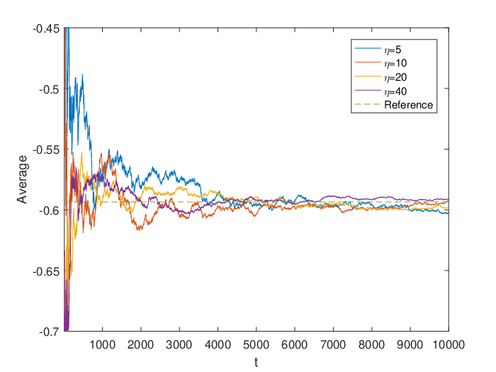
As we mentioned before in §IV.1 and also have seen in the numerical results in Figures 6 and 8, sampling of the off-diagonal observable is more challenging in PIMD-SH due to the contribution to the weight by ring polymer configurations with kinks and also the sampling variance is larger. In this test, we show that increasing the hopping intensity parameter , which makes hopping more frequent, helps sampling off-diagonal observables. For , , and , we test the PIMD-SH method with respectively till . Recall that a small time step size is required to maintain the accuracy and stability of the integrator.
The results are plotted in Figure 9 and the errors in the empirical averages together with their confidence intervals and mean squared errors are shown in Table 4. Increasing the hopping intensity parameter can effectively reduce the sampling error and variance. We admit though it is computationally more expensive to use a larger since the time step size has to be smaller by directly applying the JBAOABJ scheme. A better numerical scheme in the spirit of [42, 43] is needed and will be leaved for future works.
| Error | 8.27e-3 | 1.38e-3 | 4.97e-3 | 1.44e-3 |
| 95% C.I. | 1.09e-2 | 7.67e-3 | 3.59e-3 | 1.87e-3 |
| M.S.E. | 9.93e-5 | 1.32e-5 | 2.80e-5 | 2.98e-6 |
V Conclusion
We have proposed in this work the PIMD-SH method for sampling the thermal equilibrium average of multi-level quantum systems. The formulation is justified theoretically and supported by numerical results.
Among the possible future directions based on the current work, the most interesting direction is perhaps to combine this approach with surface hopping method for sampling dynamical correlation functions of the type , for which the ring polymer representation we developed in this work is well suited.
Better numerical integration strategies especially for using a larger hopping intensity parameter is worth exploring. Further investigation is also needed when the off-diagonal components of the potential function changes sign or takes complex values.
Acknowledgements.
This work is partially supported by the National Science Foundation under grant DMS-1454939. J.L. would like to thank Giovanni Ciccotti and John Tully for helpful discussions.Appendix A Ring polymer representations for a general two-level matrix potential
We have assumed that the off-diagonal terms of the matrix potential in a two-level system is real and does not change sign. In this Appendix, we discuss the formulations for a general two-level system. Since the potential matrix is Hermitian, the diagonal potential terms and are always real, while and may be complex with .
If we repeat the derivation in Section II.3 for the general case, everything is parallel till the step when we approximate with the Strang splitting in (16). In the general case, the off diagonal part of the matrix changes to
Using again the Strang splitting and the explicit expression of , we get (cf. (17))
| (27) |
Different from the case considered in the main text, since is complex, in general the phase factor does not cancel for all the kinks in the ring polymer. We can still approximate the partition function as an average over the extended phase space, though the quantities to be averages is now complex (in the case where the off-diagonal entry of is real but changes sign, we will need to average over terms with different signs). If we collect of the phase factors in a single term, we arrive at the following approximation
where the weight factor becomes
and , are still defined as before in (4) and (20) respectively. Recall that in the previous case, the weight factor for the partition function, corresponding to the identity operator, is just constant . As a result, the thermal average of a general observable becomes a ratio of ensemble averages
where the expression of is same as before in (5) and the equilibrium distribution is given in (8). This can still be sampled using a PIMD-SH dynamics associated with the Gibbs distribution on , though some bias will be introduced if we use the same ergodic trajectory to sample both the numerator and denominator.
Another consequence of the general phase of the term is that the partition function is determined through averaging of terms that change signs / phases, which is reminiscent of the “sign problems” in quantum Monte Carlo simulations. Further investigations of such issues are needed.
Let us remark that there are other possibilities of choosing the effective Hamiltonian and the corresponding weight functions. For example, after the splitting of , instead rewrite the and functions to the exponent, we can put these terms to the weight functions. We choose the present approach since in the case that the off-diagonal matrix potentials are real and do not change sign, it reduces to a nice probabilistic sampling problem; but for general cases, it is worth considering other approaches.
Appendix B Ring polymer representations for -level system ()
We show the extension of the ring polymer representation to a general -level system () in this Appendix. For simplicity of the presentation, let us just focus on the expression for the partition function, cf. the derivation in Section II.3; the expression for the observable follows analogously. For the -level case, The Hamiltonian is given by
where the kinetic operator is still diagonal, and the potential matrix is a Hermitian matrix such that . We decompose the matrix potential potential as follows
where is the diagonal part of and the off-diagonal part has been decomposed pairwisely into a sum of with elements given by
| (28) |
Note that in reformulating the partition function, one can still apply the Strang splitting to each and obtain (15). Next, in order to derive an approximate formula for matrix elements of , we applied the Strang splitting multiple times and get
| (29) | ||||
where the last line defines , the approximate matrix for . Here, for the diagonal part,
| (30) |
And for the off-diagonal part, we have
| (31) |
Next, we observe that
| (32) | ||||
where with each entry takes possible values in . We introduce the augmented index , and observe that when two consecutive index in are different, the product in (32) is either or gains a multiplier of order . Therefore, if we omit all the terms which are of order , we conclude that, when ,
| (33) | ||||
where
By the Taylor’s expansion, we can further simplify and obtain
| (34) |
Similarly, for , if we omit all the terms which are of order in (32), we obtain that
| (35) | ||||
Note that the two expressions above are natural generalization of the two level counterpart (17).
Appendix C Ring polymer representations for -level system in the adiabatic picture
In this section, we instead use the adiabatic basis to handle discrete electronic states, and we are able to recover the results by Schmidt and Tully in [27]. We start with (15), where the electronic states have not been specified yet. We denote the adiabatic states by and the adiabatic surface by , where , and they satisfy
| (36) |
By inserting multiple times the resolution of identity , we get
As are eigenfunctions of , , the above can be further simplified as
If we define the short hand
we obtain
| (37) |
with the effective Hamiltonian given by
This is exactly the ring polymer representation derived in [27]. The PIMD-SH sampling method can be applied to the adiabatic picture as well, which we will consider in future works.
References
- [1] N. Makri, Annu. Rev. Phys. Chem. 50, 167 (1999).
- [2] G. Stock and M. Thoss, Adv. Chem. Phys. 131, 243 (2005).
- [3] R. Kapral, Annu. Rev. Phys. Chem. 57, 129 (2006).
- [4] R. Feynman, Statistical Mechanics (Addison-Wesley, Reading, MA, 1972).
- [5] D. Chandler and P. Wolynes, J. Chem. Phys. 74, 4078 (1981).
- [6] B. Berne and D. Thirumalai, Ann. Rev. Phys. Chem. 37, 401 (1986).
- [7] T. E. Markland and D. E. Manolopoulos, J. Chem. Phys. 129, 024105 (2008).
- [8] M. Ceriotti, M. Parrinello, T. E. Markland, and D. E. Manolopoulos, J. Chem. Phys. 133, 124104 (2010).
- [9] J. Cao and G. Voth, J. Chem. Phys. 100, 5093 (1994a).
- [10] J. Cao and G. Voth, J. Chem. Phys. 100, 5106 (1994b).
- [11] S. Jang and G. A. Voth, J. Chem. Phys. 111, 2371 (1999).
- [12] I. R. Craig and D. E. Manolopoulos, J. Chem. Phys. 121, 3368 (2004).
- [13] S. Habershon, D. E. Manolopoulos, T. Markland, and T. Miller III, Annu. Rev. Phys. Chem. 64 (2013).
- [14] T. Hele, M. Willatt, A. Muolo, and S. Althorpe, J. Chem. Phys. 142, 134103 (2015a).
- [15] T. Hele, M. Willatt, A. Muolo, and S. Althorpe, J. Chem. Phys. 142, 191101 (2015b).
- [16] J. Liu, J. Chem. Phys. 140, 224107 (2014).
- [17] J. Liu and Z. Zhang, J. Chem. Phys. 144, 034307 (2016).
- [18] H.-D. Meyer and W. Miller, J. Chem. Phys. 70, 3214 (1979).
- [19] G. Stock and M. Thoss, Phys. Rev. Lett. 78, 578 (1997).
- [20] N. Ananth and T. F. Miller III, J. Chem. Phys. 133, 234103 (2010).
- [21] J. Richardson and M. Thoss, J. Chem. Phys. 139, 031102 (2013).
- [22] N. Ananth, J. Chem. Phys. 139, 124102 (2013).
- [23] A. Menzeleev, F. Bell, and M. I. T. F., J. Chem. Phys. 140, 064103 (2014).
- [24] S. Cotton and W. Miller, J. Phys. Chem. A 119, 12138 (2015).
- [25] T. Hele and N. Ananth, Farad. Discuss. (2016).
- [26] J. Liu, J. Chem. Phys. 145, 204105 (2016).
- [27] J. R. Schmidt and J. C. Tully, J. Chem. Phys. 127, 094103 (2007).
- [28] J. C. Tully, J. Chem. Phys. 93, 1061 (1990).
- [29] S. Hammes-Schiffer and J. C. Tully, J. Chem. Phys. 101, 4657 (1994).
- [30] J. C. Tully, Faraday Discussions 110, 407 (1998).
- [31] N. Shenvi, S. Roy, and J. C. Tully, Science 326, 829 (2009).
- [32] M. Barbatti, WIREs Comput. Mol. Sci. 1, 620 (2011).
- [33] J. E. Subotnik and N. Shenvi, J. Chem. Phys. 134, 024105 (2011).
- [34] J. E. Subotnik, A. Jain, B. Landry, A. Petit, W. Ouyang, and N. Bellonzi, Annu. Rev. Phys. Chem. 67, 387 (2016).
- [35] J. Lu and Z. Zhou, “Frozen Gaussian approximation with surface hopping for mixed quantum-classical dynamics: A mathematical justification of fewest switches surface hopping algorithms,” (2016a), preprint, arXiv:1602.06459.
- [36] J. Lu and Z. Zhou, J. Chem. Phys. 145, 124109 (2016b).
- [37] P. Shushkov, R. Li, and J. C. Tully, J. Chem. Phys. 137, 22A549 (2012).
- [38] J. R. Schmidt, P. V. Parandekar, and J. C. Tully, J. Chem. Phys. 129, 044104 (2008).
- [39] M. Sherman and S. Corcelli, J. Chem. Phys. 142, 024110 (2015).
- [40] G. Strang, SIAM J. Numer. Anal. 5, 506 (1968).
- [41] D. M. Ceperley, Reviews in Mineralogy and Geochemistry 71, 129 (2010).
- [42] J. Lu and E. Vanden-Eijnden, J. Chem. Phys. 138, 084105 (2013).
- [43] T.-Q. Yu, J. Lu, C. F. Abrams, and E. Vanden-Eijnden, Proc. Natl. Acad. Sci. USA 113, 11744 (2016).
- [44] B. Leimkuhler and C. Matthews, J. Chem. Phys. 138, 174102 (2013).
- [45] J. Liu, D. Li, and X. Liu, J. Chem. Phys. 145, 024103 (2016).
- [46] The work [45] actually considered two slightly different variants of BAOAB style splitting, the BAOAB splitting we use here, which is consistent with [44], corresponds to what [45] referred as BAOAB-num.