跳到论文正文
W Papers独立论文阅读器 arXiv:1701.06442 论文正文 计算阅读时间 · 0%
引用这篇论文根据当前论文元数据生成,正式投稿前建议核对。


License: arXiv.org perpetual non-exclusive license
arXiv:1701.06442v1 [math.NA] 23 Jan 2017

Dimension and basis construction for analysis-suitable
G1G^{1} two-patch parameterizations

Mario Kapl Email: mario.kapl@unipv.it Address: Dipartimento di Matematica “F.Casorati", Università degli Studi di Pavia, Italy Corresponding author: Corresponding author    Giancarlo Sangalli Email: giancarlo.sangalli@unipv.it Address: Dipartimento di Matematica “F.Casorati", Università degli Studi di Pavia, Italy Address: Istituto di Matematica Applicata e Tecnologie Informatiche ”E.Magenes“ (CNR), Italy    Thomas Takacs Email: thomas.takacs@jku.at Address: Institute of Applied Geometry, Johannes Kepler University Linz, Austria
Abstract

We study the dimension and construct a basis for C1C^{1}-smooth isogeometric function spaces over two-patch domains. In this context, an isogeometric function is a function defined on a B-spline domain, whose graph surface also has a B-spline representation. We consider constructions along one interface between two patches. We restrict ourselves to a special case of planar B-spline patches of bidegree (p,p)(p,p) with p≥3p\geq 3, so-called analysis-suitable G1G^{1} geometries, which are derived from a specific geometric continuity condition. This class of two-patch geometries is exactly the one which allows, under certain additional assumptions, C1C^{1} isogeometric spaces with optimal approximation properties (cf. [9]).

Such spaces are of interest when solving numerically fourth-order PDE problems, such as the biharmonic equation, using the isogeometric method. In particular, we analyze the dimension of the C1C^{1}-smooth isogeometric space and present an explicit representation for a basis of this space. Both the dimension of the space and the basis functions along the common interface depend on the considered two-patch parameterization. Such an explicit, geometry dependent basis construction is important for an efficient implementation of the isogeometric method. The stability of the constructed basis is numerically confirmed for an example configuration.

Keywords: 
isogeometric analysis , analysis-suitable G1G^{1} geometries , C1C^{1} smooth isogeometric functions , geometric continuity

1 Introduction

The problems discussed in this paper are inspired by isogeometric analysis (IGA), which was developed in [15]. The core idea of isogeometric analysis is to use the spline based representation of CAD models directly for the numerical analysis of partial differential equations (PDE). For a more detailed description of the isogeometric framework we refer to [3, 10].

One of the advantages of IGA is the possibility to have discretization spaces of high order smoothness. These spaces can then be used to directly solve high order PDE problems. There exist several fourth (and higher) order problems of practical relevance. For their application in IGA see [2, 31], as well as [1, 4, 5, 19, 20] for Kirchhoff-Love shells, [12] for the Cahn-Hilliard equation and [13] for the Navier-Stokes-Korteweg equation.

The spline based representation of the physical domains allows for high order smoothness within one B-spline patch. However, most geometries of practical relevance cannot be represented directly with one patch but have to be parametrized using a multi-patch approach. It is not trivial to construct smooth function spaces over multi-patch domains. Many results for multi-patch domains can be derived from considerations on a single interface, hence in the following we will restrict ourselves to two-patch domains.

We are interested in C1C^{1} isogeometric function spaces over two-patch domains. More precisely, we compute the dimension and construct a stable basis for a special class of, so called, analysis-suitable G1G^{1} parameterizations. This class of geometries was first introduced in [9], where it was also shown that exactly the geometries of this class allow under certain assumptions C1C^{1} isogeometric spaces with optimal approximation properties (cf. [9]). Note that an isogeometric function is C1C^{1} if its graph surface is G1G^{1}. Hence, the analysis-suitability condition is a restriction of the more general geometric continuity condition. We refer to [24, 27] for the definition of geometric continuity.

The existing literature about the construction of C1C^{1}-smooth isogeometric functions on two-patch (and multi-patch) domains can be roughly classified into two possible approaches. The first one employs G1G^{1}-surface constructions around extraordinary vertices to obtain a set of C1C^{1}-smooth functions, see e.g. [18, 24, 25, 26]. In contrast, the second approach studies the entire space of C1C^{1}-smooth isogeometric functions on any given two-patch (or multi-patch) parameterization and generate a basis of the corresponding C1C^{1} isogeometric space. Examples are [6, 9, 16, 17, 22, 23].

In this paper we follow the second approach, especially explored in [6, 16, 17, 22]. We extend these results in two main directions. First, these existing constructions and investigations are limited to piecewise bilinear domains. Our approach encloses the much wider class of analysis-suitable G1G^{1} parameterizations, which contains the class of piecewise bilinear domains. Second, our construction works for non-uniform splines of arbitrary bidegree (p,p)(p,p) with p≥3p\geq 3 and of arbitrary regularity rr with 1≤r<p−11\leq r<p-1 within the two single patches. In contrast, the constructions [6, 22] are restricted to biquartic (for special cases) and to biquintic Bézier elements and the constructions [16, 17] are restricted to bicubic and biquartic uniform splines of regularity r=1r=1.

Further differences to [6, 22] are that our approach allows the construction of nested C1C^{1} isogeometric spaces and that our basis functions are explicitly given, whereas the basis functions in [6, 22] are implicitly defined by means of minimal determining sets for the Bézier coefficients. Similar to [16, 17], the explicitly given basis functions possess a very small local support and are well conditioned. Moreover, the spline coefficients of our basis functions can be simply obtained by means of blossoming or fitting. This could provide a simple implementation in existing IGA libraries. In addition, we present the study of the dimension of the resulting C1C^{1} isogeometric spaces for all possible configurations of analysis-suitable G1G^{1} two-patch parameterizations.

The remainder of the paper is organized as follows. In Section 2 we describe some basic definitions and notations which are used throughout the paper. Section 3 recalls the concept of C1C^{1}-smooth isogeometric spaces over analysis-suitable G1G^{1} two-patch parameterizations. The dimension of these spaces, which depends on the considered two-patch parameterization, is analyzed in Section 4. Then we present in Section 5 an explicit construction of basis functions, and describe in Section 6 their resulting spline coefficients by means of blossoming (and fitting). Finally, we conclude the paper in Section 7.

2 Preliminaries

Let ω\omega be the interval [0,1][0,1] or the unit square [0,1]2[0,1]^{2}. We denote by 𝒮⁡(𝒯kp,r,ω)\mathcal{S}(\mathcal{T}^{p,r}_{k},\omega) the (tensor-product) spline space of degree pp (in each direction), which is defined on ω\omega by choosing the open knot vector 𝒯kp,r=(t0p,r,…,t2​p+1+k⁡(p−r)p,r)\mathcal{T}^{p,r}_{k}=(t^{p,r}_{0},\ldots,t^{p,r}_{2p+1+k(p-r)}) (in each direction) given by

𝒯kp,r=(0,…,0⏟(p+1)−times,τ1,…,τ1⏟(p−r)−times,τ2,…,τ2⏟(p−r)−times,…,τk,…,τk⏟(p−r)−times,1,…,1⏟(p+1)−times),\mathcal{T}^{p,r}_{k}=(\underbrace{0,\ldots,0}_{(p+1)-\mbox{\scriptsize times}},\underbrace{\textstyle\tau_{1},\ldots,\tau_{1}}_{(p-r)-\mbox{\scriptsize times}},\underbrace{\textstyle\tau_{2},\ldots,\tau_{2}}_{(p-r)-\mbox{\scriptsize times}},\ldots,\underbrace{\textstyle\tau_{k},\ldots,\tau_{k}}_{(p-r)-\mbox{\scriptsize times}},\underbrace{1,\ldots,1}_{(p+1)-\mbox{\scriptsize times}}),

where k∈ℕ0k\in\mathbb{N}_{0}, 0<τi<τi+1<10<\tau_{i}<\tau_{i+1}<1 for all 1≤i≤k−11\leq i\leq k-1 and kk is the number of different inner knots (in each direction). Thereby rr describes the resulting CrC^{r}-continuity of the space 𝒮⁡(𝒯kp,r,ω)\mathcal{S}(\mathcal{T}^{p,r}_{k},\omega) at all inner knots. The range for the regularity parameter rr is in general 0≤r≤p−10\leq r\leq p-1. However, the focus here is on r≥1r\geq 1. Of course, in case of tensor-product splines, the knot vectors could be different in each direction. Moreover, the knot multiplicities could be different for every knot. To keep the presentation simple, we consider only the presented case. The spline spaces 𝒮⁡(𝒯kp,r,[0,1])\mathcal{S}(\mathcal{T}^{p,r}_{k},[0,1]) and 𝒮⁡(𝒯kp,r,[0,1]2)\mathcal{S}(\mathcal{T}^{p,r}_{k},[0,1]^{2}) are spanned by the (tensor-product) B-splines Nip,rN^{p,r}_{i} and Ni,jp,r=Nip,r​Njp,rN_{i,j}^{p,r}=N_{i}^{p,r}N_{j}^{p,r}, i,j=0,…,p+k⁡(p−r)i,j=0,\ldots,p+k(p-r), respectively. Each function h∈𝒮⁡(𝒯kp,r,[0,1])h\in\mathcal{S}(\mathcal{T}^{p,r}_{k},[0,1]) and z∈𝒮⁡(𝒯kp,r,[0,1]2)z\in\mathcal{S}(\mathcal{T}^{p,r}_{k},[0,1]^{2}) possesses a B-spline representation

h⁡(t)=∑i=0p+k⁡(p−r)di​Nip,r​(t)h(t)=\sum_{i=0}^{p+k(p-r)}d_{i}N_{i}^{p,r}(t) (1)

and

z⁡(u,v)=∑i=0p+k⁡(p−r)∑j=0p+k⁡(p−r)di,j​Ni,jp,r​(u,v)z(u,v)=\sum_{i=0}^{p+k(p-r)}\sum_{j=0}^{p+k(p-r)}d_{i,j}N_{i,j}^{p,r}(u,v)

with spline control points di∈ℝd_{i}\in\mathbb{R} and di,j∈ℝd_{i,j}\in\mathbb{R}, respectively.

In addition, we consider the knot vectors 𝒯k,ℓp,r=(t0p,r,…,t2​p+2+k⁡(p−r)p,r)\mathcal{T}^{p,r}_{k,\ell}=(t^{p,r}_{0},\ldots,t^{p,r}_{2p+2+k(p-r)}) and 𝒯k,ℓ,ℓ′p,r=(t0p,r,…,t2​p+3+k⁡(p−r)p,r)\mathcal{T}^{p,r}_{k,\ell,\ell^{\prime}}=(t^{p,r}_{0},\ldots,t^{p,r}_{2p+3+k(p-r)}), which are obtained by inserting into the knot vector 𝒯kp,r\mathcal{T}^{p,r}_{k} the knot τℓ\tau_{\ell} with the index ℓ∈{1,…,k}\ell\in\{1,\ldots,k\} (in case of 𝒯k,ℓp,r\mathcal{T}^{p,r}_{k,\ell}) and the knots τℓ\tau_{\ell} and τℓ′\tau_{\ell^{\prime}} with the indices ℓ,ℓ′∈{1,…,k}\ell,\ell^{\prime}\in\{1,\ldots,k\} and ℓ≠ℓ′\ell\neq\ell^{\prime} (in case of OPEN𝒯k,ℓ,ℓ′p,r)\mathcal{T}^{p,r}_{k,\ell,\ell^{\prime}}). The resulting spline spaces are denoted by 𝒮⁡(𝒯k,ℓp,r,ω)\mathcal{S}(\mathcal{T}^{p,r}_{k,\ell},\omega) and 𝒮⁡(𝒯k,ℓ,ℓ′p,r,ω)\mathcal{S}(\mathcal{T}^{p,r}_{k,\ell,\ell^{\prime}},\omega), respectively, and are again CrC^{r}-smooth at all inner knots except at the knot τℓ\tau_{\ell} or at the knots τℓ\tau_{\ell}, τℓ′\tau_{\ell^{\prime}}, respectively, where the spaces are only Cr−1C^{r-1}-smooth. Moreover, we denote by 𝒫p​(ω)\mathcal{P}^{p}(\omega) the space of (tensor-product) polynomials of degree pp on ω\omega.

3 C1C^{1}-smooth isogeometric spaces and AS G1G^{1} two-patch geometries

We consider a planar domain Ω⊂ℝ2\Omega\subset\mathbb{R}^{2} composed of two quadrilateral spline patches Ω(L)\Omega^{(L)} and Ω(R)\Omega^{(R)}, i.e. Ω=Ω(L)∪Ω(R)\Omega=\Omega^{(L)}\cup\Omega^{(R)}, which share a whole edge as common interface Γ=Ω(L)∩Ω(R)\Gamma=\Omega^{(L)}\cap\Omega^{(R)}. We assume that each patch Ω(S)\Omega^{(S)}, S∈{L,R}S\in\{L,R\}, is the image 𝑭(S)​([0,1]2)\boldsymbol{F}^{(S)}([0,1]^{2}) of a regular, bijective geometry mapping

𝑭(S):[0,1]2→Ω(S),𝑭(S)∈𝒮⁡(𝒯kp,r,[0,1]2),\boldsymbol{F}^{(S)}:[0,1]^{2}\rightarrow\Omega^{(S)},\quad\boldsymbol{F}^{(S)}\in\mathcal{S}(\mathcal{T}^{p,r}_{k},[0,1]^{2}),

with the spline representations

𝑭(S)​(u,v)=∑i=0p+k⁡(p−r)∑j=0p+k⁡(p−r)𝒄i,j(S)​Ni,jp,r​(u,v),𝒄i,j(S)∈ℝ2.\boldsymbol{F}^{(S)}(u,v)=\sum_{i=0}^{p+k(p-r)}\sum_{j=0}^{p+k(p-r)}\boldsymbol{c}^{(S)}_{i,j}N_{i,j}^{p,r}(u,v),\quad\boldsymbol{c}^{(S)}_{i,j}\in\mathbb{R}^{2}.

For the sake of simplicity, we assume that the two patches 𝑭(L)\boldsymbol{F}^{(L)} and 𝑭(R)\boldsymbol{F}^{(R)} share the common interface at

𝑭(L)​(0,v)=𝑭(R)​(0,v),v∈[0,1].\boldsymbol{F}^{(L)}(0,v)=\boldsymbol{F}^{(R)}(0,v),\quad v\in[0,1].

We denote the parameterization of the common curve at Γ\Gamma by 𝑭0:[0,1]→ℝ2\boldsymbol{F}_{0}:[0,1]\rightarrow\mathbb{R}^{2} and assume that 𝑭0​(v)=𝑭(L)​(0,v)=𝑭(R)​(0,v)\boldsymbol{F}_{0}(v)=\boldsymbol{F}^{(L)}(0,v)=\boldsymbol{F}^{(R)}(0,v). The space of isogeometric functions on Ω\Omega is given as

𝒱={ϕ:Ω→ℝ such that ϕ∘𝑭(S)∈𝒮(𝒯kp,r,[0,1]2), S∈{L,R}}.\mathcal{V}=\{\phi:\Omega\rightarrow\mathbb{R}\mbox{ such that }\phi\circ\boldsymbol{F}^{(S)}\in\mathcal{S}(\mathcal{T}^{p,r}_{k},[0,1]^{2}),\mbox{ }S\in\{L,R\}\}.

The graph surface 𝚺⊂Ω×ℝ\boldsymbol{\Sigma}\subset\Omega\times\mathbb{R} of an isogeometric function ϕ∈𝒱\phi\in\mathcal{V} consists of the two graph surface patches

𝚺(S):[0,1]2→Ω(S)×ℝ,S∈{L,R},\boldsymbol{\Sigma}^{(S)}:[0,1]^{2}\rightarrow\Omega^{(S)}\times\mathbb{R},\quad S\in\{L,R\},

possessing the form

𝚺(S)​(u,v)=(𝑭(S)​(u,v),g(S)​(u,v))T,\boldsymbol{\Sigma}^{(S)}(u,v)=(\boldsymbol{F}^{(S)}(u,v),g^{(S)}(u,v))^{T},

where g(S)=ϕ∘𝑭(S)∈𝒮⁡(𝒯kp,r,[0,1]2)g^{(S)}=\phi\circ\boldsymbol{F}^{(S)}\in\mathcal{S}(\mathcal{T}^{p,r}_{k},[0,1]^{2}). Since the geometry mappings 𝑭(S)\boldsymbol{F}^{(S)}, S∈{L,R}S\in\{L,R\}, are given, an isogeometric function ϕ∈𝒱\phi\in\mathcal{V} is determined by the two associated spline functions g(S)g^{(S)}, S∈{L,R}S\in\{L,R\}, with the spline representations

g(S)​(u,v)=∑i=0p+k⁡(p−r)∑j=0p+k⁡(p−r)di,j(S)​Ni,jp,r​(u,v),di,j(S)∈ℝ.g^{(S)}(u,v)=\sum_{i=0}^{p+k(p-r)}\sum_{j=0}^{p+k(p-r)}d^{(S)}_{i,j}N_{i,j}^{p,r}(u,v),\quad d^{(S)}_{i,j}\in\mathbb{R}.

We are interested in C1C^{1}-smooth isogeometric functions ϕ∈𝒱\phi\in\mathcal{V}. We assume C0C^{0}-smoothness condition of ϕ\phi, that results in

g(L)​(0,v)=g(R)​(0,v),g^{(L)}(0,v)=g^{(R)}(0,v), (2)

for v∈[0,1]v\in[0,1]. We denote the function along the common interface by g⁡(v)=g(L)​(0,v)=g(R)​(0,v)g(v)=g^{(L)}(0,v)=g^{(R)}(0,v). Let us consider the space 𝒱1\mathcal{V}^{1} of C1C^{1}-smooth isogeometric functions on Ω\Omega, i.e.

𝒱1=𝒱∩C1​(Ω),\mathcal{V}^{1}=\mathcal{V}\cap C^{1}(\Omega),

in more detail. An isogeometric function ϕ∈𝒱\phi\in\mathcal{V} belongs to 𝒱1\mathcal{V}^{1} if and only if the two graph surface patches 𝚺(L)\boldsymbol{\Sigma}^{(L)} and 𝚺(R)\boldsymbol{\Sigma}^{(R)} possess a well defined tangent plane along the common interface 𝚺(L)∩𝚺(R)\boldsymbol{\Sigma}^{(L)}\cap\boldsymbol{\Sigma}^{(R)}, compare [9, 16, 17]. This is equivalent to the condition that there exist functions α(L),α(R),β:[0,1]→ℝ\alpha^{(L)},\alpha^{(R)},\beta:[0,1]\rightarrow\mathbb{R} such that for all v∈[0,1]v\in[0,1]

α(L)​(v)​α(R)​(v)<0\alpha^{(L)}(v)\alpha^{(R)}(v)<0 (3)

and

α(R)​(v)​Du​𝚺(L)​(0,v)−α(L)​(v)​Du​𝚺(R)​(0,v)+β⁡(v)​Dv​𝚺(R)​(0,v)=𝟎,\alpha^{(R)}(v)D_{u}\boldsymbol{\Sigma}^{(L)}(0,v)-\alpha^{(L)}(v)D_{u}\boldsymbol{\Sigma}^{(R)}(0,v)+\beta(v)D_{v}\boldsymbol{\Sigma}^{(R)}(0,v)=\boldsymbol{0}, (4)

see [28]. The above described equivalent conditions are called geometric continuity of order 11 or G1G^{1}-smoothness (cf. [14, 28]).

Note that the first two equations (4), i.e.

α(R)​(v)​Du​𝑭(L)​(0,v)−α(L)​(v)​Du​𝑭(R)​(0,v)+β⁡(v)​Dv​𝑭0​(v)=𝟎,\alpha^{(R)}(v)D_{u}\boldsymbol{F}^{(L)}(0,v)-\alpha^{(L)}(v)D_{u}\boldsymbol{F}^{(R)}(0,v)+\beta(v)D_{v}\boldsymbol{F}_{0}(v)=\boldsymbol{0}, (5)

uniquely determine the functions α(L)\alpha^{(L)}, α(R)\alpha^{(R)} and β\beta up to a common function γ:[0,1]→ℝ\gamma:[0,1]\rightarrow\mathbb{R} (with γ⁡(v)≠0\gamma(v)\neq 0) by

α(L)=γ⁡(v)​α¯(L),α(R)=γ⁡(v)​α¯(R)​ and ​β​(v)=γ⁡(v)​β¯​(v),\alpha^{(L)}=\gamma(v)\bar{\alpha}^{(L)},\alpha^{(R)}=\gamma(v)\bar{\alpha}^{(R)}\mbox{ and }\beta(v)=\gamma(v)\bar{\beta}(v), (6)

where

α¯(S)(v)=det(Du𝑭(S)(0,v),Dv𝑭0(v)), S∈{L,R},\bar{\alpha}^{(S)}(v)=\det(D_{u}\boldsymbol{F}^{(S)}(0,v),D_{v}\boldsymbol{F}_{0}(v)),\mbox{ }S\in\{L,R\}, (7)

and

β¯​(v)=det(Du​𝑭(L)​(0,v),Du​𝑭(R)​(0,v)),\bar{\beta}(v)=\det(D_{u}\boldsymbol{F}^{(L)}(0,v),D_{u}\boldsymbol{F}^{(R)}(0,v)), (8)

see e.g. [9, 28].

Therefore, an isogeometric function ϕ∈𝒱\phi\in\mathcal{V} belongs to 𝒱1\mathcal{V}^{1} if and only if the equation

α(R)​(v)​Du​g(L)​(0,v)−α(L)​(v)​Du​g(R)​(0,v)+β⁡(v)​Dv​g​(v)=0\alpha^{(R)}(v)D_{u}g^{(L)}(0,v)-\alpha^{(L)}(v)D_{u}g^{(R)}(0,v)+\beta(v)D_{v}g(v)=0 (9)

is satisfied for all v∈[0,1]v\in[0,1]. Equations (2) and (9) lead to linear constraints on the spline control points di,j(S)d_{i,j}^{(S)} of g(S)g^{(S)}, S∈{L,R}S\in\{L,R\}, with indices (S,i,j)(S,i,j) belonging to the index space

IΓ={(S,i,j) | S∈{L,R}, i=0,1 and j=0,…,p+k(p−r)}.I_{\Gamma}=\{(S,i,j)\mbox{ }|\mbox{ }S\in\{L,R\},\mbox{ }i=0,1\mbox{ and }j=0,\ldots,p+k(p-r)\}.

Moreover, we denote by II the index space formed by all spline control points di,j(S)d_{i,j}^{(S)}, S∈{L,R}S\in\{L,R\}, i.e.

I={(S,i,j) | S∈{L,R} and i,j=0,…,p+k(p−r)}.I=\{(S,i,j)\mbox{ }|\mbox{ }S\in\{L,R\}\mbox{ and }i,j=0,\ldots,p+k(p-r)\}.

Furthermore, for functions α(L),α(R)\alpha^{(L)},\alpha^{(R)} and β\beta satisfying equations (5) there exist non-unique functions β(L),β(R):[0,1]→ℝ\beta^{(L)},\beta^{(R)}:[0,1]\rightarrow\mathbb{R} such that

β⁡(v)=α(L)​(v)​β(R)​(v)−α(R)​(v)​β(L)​(v),\beta(v)=\alpha^{(L)}(v)\beta^{(R)}(v)-\alpha^{(R)}(v)\beta^{(L)}(v), (10)

see e.g. [9, 28].

Note that for generic patches 𝑭(L),𝑭(R)∈𝒮⁡(𝒯kp,r,[0,1]2)\boldsymbol{F}^{(L)},\boldsymbol{F}^{(R)}\in\mathcal{S}(\mathcal{T}^{p,r}_{k},[0,1]^{2}) the functions α(L),α(R)\alpha^{(L)},\alpha^{(R)} and β\beta fulfill α(L),α(R)∈𝒮⁡(𝒯k2​p−1,r−1,[0,1])\alpha^{(L)},\alpha^{(R)}\in\mathcal{S}(\mathcal{T}^{2p-1,r-1}_{k},[0,1]) as well as β∈𝒮⁡(𝒯k2​p,r,[0,1])\beta\in\mathcal{S}(\mathcal{T}^{2p,r}_{k},[0,1]). For special configurations the degree may be lower and the regularity may be higher.

Motivated by [9, 28], we restrict in the following the considered geometry mappings 𝑭(L)\boldsymbol{F}^{(L)} and 𝑭(R)\boldsymbol{F}^{(R)} to geometry mappings possessing linear functions α(L)\alpha^{(L)}, α(R)\alpha^{(R)}, β(L)\beta^{(L)}, β(R)\beta^{(R)}, as stated in the following definition.

Definition 1 (Analysis-suitable G1G^{1}, cf. [9]).

The two-patch geometry parameterization 𝑭(L)\boldsymbol{F}^{(L)} and 𝑭(R)\boldsymbol{F}^{(R)} is analysis-suitable G1G^{1} (AS G1G^{1}) if there exist α(L)\alpha^{(L)}, α(R)\alpha^{(R)}, β(L)\beta^{(L)}, β(R)∈𝒫1​([0,1])\beta^{(R)}\in\mathcal{P}^{1}([0,1]), with α(L)\alpha^{(L)} and α(R)\alpha^{(R)} relatively prime (i.e., deg⁡(gcd⁡(α(L),α(R)))=0\deg(\gcd(\alpha^{(L)},\alpha^{(R)}))=0) satisfying equations (5) and (10).

The condition on deg⁡(gcd⁡(α(L),α(R)))=0\deg(\gcd(\alpha^{(L)},\alpha^{(R)}))=0 was not used in [9] but is not restrictive: if deg⁡(gcd⁡(αL,αR))=1\deg(\gcd(\alpha^{L},\alpha^{R}))=1 one can replace α(L)\alpha^{(L)}, α(R)\alpha^{(R)} and β\beta by α(L)/gcd⁡(α(L),α(R))\alpha^{(L)}/\gcd(\alpha^{(L)},\alpha^{(R)}), α(R)/gcd⁡(α(L),α(R))\alpha^{(R)}/\gcd(\alpha^{(L)},\alpha^{(R)}) and β/gcd⁡(α(L),α(R))\beta/\gcd(\alpha^{(L)},\alpha^{(R)}), respectively. Obviously, the polynomial β\beta is divisible by gcd⁡(α(L),α(R))\gcd(\alpha^{(L)},\alpha^{(R)}), which can be seen best in (10). With deg⁡(gcd⁡(α(L),α(R)))=0\deg(\gcd(\alpha^{(L)},\alpha^{(R)}))=0, the functions α(L)\alpha^{(L)}, α(R)\alpha^{(R)} and β\beta are uniquely determined up to a common constant.

It was shown in [9] when the functions α(S)\alpha^{(S)} and β(S)\beta^{(S)}, S∈{L,R}S\in\{L,R\}, are assumed to be of higher degree or even to be spline functions along the interface, then the polynomial representation along the interface is reduced to lower degrees. Hence, these spaces do not guarantee optimal approximation order. For this more general case the investigation of a dimension formula or of a basis construction should be possible in similar way as presented in the following sections, but is beyond the scope of this paper.

4 Dimension of the space 𝒱1\mathcal{V}^{1} for AS G1G^{1} two-patch geometries

We consider AS G1G^{1} geometries 𝑭(L),𝑭(R)∈𝒮⁡(𝒯kp,r,[0,1]2)\boldsymbol{F}^{(L)},\boldsymbol{F}^{(R)}\in\mathcal{S}(\mathcal{T}^{p,r}_{k},[0,1]^{2}) with the corresponding functions α(L)\alpha^{(L)}, α(R)∈𝒫1​([0,1])\alpha^{(R)}\in\mathcal{P}^{1}([0,1]) and β∈𝒫2​([0,1])\beta\in\mathcal{P}^{2}([0,1]).

Let dαd_{\alpha} be the maximum degree of the functions α(S)\alpha^{(S)}, i.e.

dα=max⁡(deg⁡(α(L)),deg⁡(α(R))).d_{\alpha}=\max(\deg(\alpha^{(L)}),\deg(\alpha^{(R)})).

Here we consider the actual degree of the functions. Since α(L),α(R)∈𝒫1​([0,1])\alpha^{(L)},\alpha^{(R)}\in\mathcal{P}^{1}([0,1]), we obtain either dα=0d_{\alpha}=0 or dα=1d_{\alpha}=1. Let zβz_{\beta} be defined as the number of different inner knots where the function β\beta possesses the value zero, i.e.

zβ=|{v0∈{τ1,…,τk} | β(v0)=0}|.z_{\beta}=|\{v_{0}\in\{\tau_{1},\ldots,\tau_{k}\}\mbox{ }|\mbox{ }\beta(v_{0})=0\}|.

Since β∈𝒫2​([0,1])\beta\in\mathcal{P}^{2}([0,1]), zβ∈{0,1,2,k}z_{\beta}\in\{0,1,2,k\}.

Depending on β\beta, we define a new knot vector 𝒯kp~\widetilde{\mathcal{T}^{p}_{k}}. First, if β=0{\beta}=0 then 𝒯kp~=𝒯kp,r\widetilde{\mathcal{T}^{p}_{k}}=\mathcal{T}^{p,r}_{k}. Otherwise, assuming β≠0{\beta}\neq 0, we have three cases: if zβ=0z_{\beta}=0, we set 𝒯kp~=𝒯kp,r+1\widetilde{\mathcal{T}^{p}_{k}}=\mathcal{T}^{p,r+1}_{k}, if zβ=1z_{\beta}=1 or zβ=2z_{\beta}=2, we set 𝒯kp~=𝒯k,ℓp,r+1\widetilde{\mathcal{T}^{p}_{k}}=\mathcal{T}^{p,r+1}_{k,\ell} or 𝒯kp~=𝒯k,ℓ,ℓ′p,r+1\widetilde{\mathcal{T}^{p}_{k}}=\mathcal{T}^{p,r+1}_{k,\ell,\ell^{\prime}}, respectively, where ℓ,∈{1,…,k}\ell,\in\{1,\ldots,k\}, and possibly ℓ′∈{1,…,k}\ell^{\prime}\in\{1,\ldots,k\} with ℓ≠ℓ′\ell\neq\ell^{\prime}, are the indices of τℓ\tau_{\ell} and τℓ′\tau_{\ell^{\prime}}, which are roots of β\beta.

We are interested in the dimension of the isogeometric space 𝒱1\mathcal{V}^{1}. Clearly, the space 𝒱1\mathcal{V}^{1} is the direct sum of the two subspaces

𝒱11={ϕ∈𝒱1 | di,j(S)=0 for S∈{L,R} and (S,i,j)∈IΓ}\mathcal{V}^{1}_{1}=\{\phi\in\mathcal{V}^{1}\mbox{ }|\mbox{ }d_{i,j}^{(S)}=0\mbox{ for }S\in\{L,R\}\mbox{ and }(S,i,j)\in I_{\Gamma}\}

and

𝒱21={ϕ∈𝒱1 | di,j(S)=0 for S∈{L,R} and (S,i,j)∈I∖IΓ},\mathcal{V}^{1}_{2}=\{\phi\in\mathcal{V}^{1}\mbox{ }|\mbox{ }d_{i,j}^{(S)}=0\mbox{ for }S\in\{L,R\}\mbox{ and }(S,i,j)\in I\setminus I_{\Gamma}\},

which implies that

dim𝒱1=dim𝒱11+dim𝒱21.\dim\mathcal{V}^{1}=\dim\mathcal{V}^{1}_{1}+\dim\mathcal{V}^{1}_{2}.

In [17], the functions of 𝒱11\mathcal{V}^{1}_{1} and 𝒱21\mathcal{V}^{1}_{2} have been called basis functions of the first and second kind, respectively. We first state the dimension of 𝒱11\mathcal{V}^{1}_{1}.

Lemma 2.

The dimension of 𝒱11\mathcal{V}^{1}_{1} is equal to

dimV11=2​(p+k⁡(p−r)−1)​(p+k⁡(p−r)+1).\dim V^{1}_{1}=2(p+k(p-r)-1)(p+k(p-r)+1).
Proof.

Clearly, dim𝒱11\dim\mathcal{V}^{1}_{1} is equal to the number of control points di,j(S)d^{(S)}_{i,j}, S∈{L,R}S\in\{L,R\}, possessing indices (S,i,j)∈I∖IΓ(S,i,j)\in I\setminus I_{\Gamma}, i.e. dim𝒱11=|I∖IΓ|\dim\mathcal{V}^{1}_{1}=|I\setminus I_{\Gamma}|. ∎

To analyze the dimension of 𝒱21\mathcal{V}^{1}_{2}, we need additional tools describing the situation at Γ\Gamma. Some of these tools have been (similarly) introduced in [9]. Consider the transversal vector 𝒅(S)\boldsymbol{d}^{(S)} defined on Γ\Gamma such that

𝒅(S)∘𝑭0(v)=(Du𝑭(S)(0,v),Dv𝑭0(v))(1,−β(S)(v))T1α(S)​(v), S∈{L,R}.\boldsymbol{d}^{(S)}\circ\boldsymbol{F}_{0}(v)=(D_{u}\boldsymbol{F}^{(S)}(0,v),D_{v}\boldsymbol{F}_{0}(v))(1,-\beta^{(S)}(v))^{T}\frac{1}{\alpha^{(S)}(v)},\mbox{ }S\in\{L,R\}.

Observe that 𝒅(L)=𝒅(R)\boldsymbol{d}^{(L)}=\boldsymbol{d}^{(R)} (which is equivalent to (5)) and therefore we simply set

𝒅=𝒅(L)=𝒅(R).\boldsymbol{d}=\boldsymbol{d}^{(L)}=\boldsymbol{d}^{(R)}.

In addition, we consider the space of traces and transversal derivatives on Γ\Gamma and its pullback, which are given by

𝒱Γ1={Γ∋(x,y)↦(ϕ(x,y),∇ϕ(x,y)⋅𝒅(x,y)), such that ϕ∈𝒱21}\mathcal{V}^{1}_{\Gamma}=\{\Gamma\ni(x,y)\mapsto(\phi(x,y),\nabla\phi(x,y)\cdot\boldsymbol{d}(x,y)),\mbox{ such that }\phi\in\mathcal{V}^{1}_{2}\}

and

𝒱Γ1^={(ϕ,∇ϕ⋅𝒅)∘𝑭0, such that ϕ∈𝒱21},\widehat{\mathcal{V}^{1}_{\Gamma}}=\{(\phi,\nabla\phi\cdot\boldsymbol{d})\circ\boldsymbol{F}_{0},\mbox{ such that }\phi\in\mathcal{V}^{1}_{2}\},

respectively. The transversal vector 𝒅\boldsymbol{d}, 𝒱Γ1\mathcal{V}^{1}_{\Gamma} and 𝒱Γ1^\widehat{\mathcal{V}^{1}_{\Gamma}} depend only on the choice of β(L)\beta^{(L)} and β(R)\beta^{(R)}, since α(L)\alpha^{(L)} and α(R)\alpha^{(R)} are now uniquely determined by the geometry mappings 𝑭(L)\boldsymbol{F}^{(L)} and 𝑭(R)\boldsymbol{F}^{(R)}. Associated to 𝒅\boldsymbol{d}, we consider the transversal derivative of ϕ\phi with respect to 𝒅\boldsymbol{d} on Γ\Gamma, i.e. (∇ϕ⋅𝒅)∘𝑭0(\nabla\phi\cdot\boldsymbol{d})\circ\boldsymbol{F}_{0}.

Clearly, for ϕ∈𝒱21\phi\in\mathcal{V}_{2}^{1} the function ϕ∘𝑭0\phi\circ\boldsymbol{F}_{0} is a spline function. More precisely, we have:

Lemma 3.

If ϕ∈𝒱21\phi\in\mathcal{V}^{1}_{2}, then ϕ∘𝐅0∈𝒮⁡(𝒯kp~,[0,1])\phi\circ\boldsymbol{F}_{0}\in\mathcal{S}(\widetilde{\mathcal{T}^{p}_{k}},[0,1]).

Proof.

Analyzing equation (9), we observe that ϕ∘𝑭0∈𝒮⁡(𝒯kp~,[0,1])\phi\circ\boldsymbol{F}_{0}\in\mathcal{S}(\widetilde{\mathcal{T}^{p}_{k}},[0,1]), since Du​g(S)​(0,v)∈𝒮⁡(𝒯kp,r,[0,1])D_{u}g^{(S)}(0,v)\in\mathcal{S}(\mathcal{T}^{p,r}_{k},[0,1]). ∎

The following lemma ensures that for ϕ∈𝒱21\phi\in\mathcal{V}_{2}^{1} the function (∇ϕ⋅𝒅)∘𝑭0(\nabla\phi\cdot\boldsymbol{d})\circ\boldsymbol{F}_{0} is a spline function, too.

Lemma 4.

If ϕ∈𝒱21\phi\in\mathcal{V}^{1}_{2}, then (∇ϕ⋅𝐝)∘𝐅0∈𝒮(𝒯kp−dα,r−1,[0,1])(\nabla\phi\cdot\boldsymbol{d})\circ\boldsymbol{F}_{0}\in\mathcal{S}(\mathcal{T}^{p-d_{\alpha},r-1}_{k},[0,1]).

Proof.

Recall that 𝒅∘𝑭0​(v)=𝒅(L)∘𝑭0​(v)=𝒅(R)∘𝑭0​(v)\boldsymbol{d}\circ\boldsymbol{F}_{0}(v)=\boldsymbol{d}^{(L)}\circ\boldsymbol{F}_{0}(v)=\boldsymbol{d}^{(R)}\circ\boldsymbol{F}_{0}(v). An isogeometric function ϕ\phi belong to the space 𝒱21\mathcal{V}^{1}_{2} if and only if

(∇(L)ϕ⋅𝒅)∘𝑭0(v)=(∇(R)ϕ⋅𝒅)∘𝑭0(v)=(∇ϕ⋅𝒅)∘𝑭0(v)(\nabla^{(L)}\phi\cdot\boldsymbol{d})\circ\boldsymbol{F}_{0}(v)=(\nabla^{(R)}\phi\cdot\boldsymbol{d})\circ\boldsymbol{F}_{0}(v)=(\nabla\phi\cdot\boldsymbol{d})\circ\boldsymbol{F}_{0}(v)

for all v∈[0,1]v\in[0,1]. Since

(∇(S)ϕ⋅𝒅)∘𝑭0(v)=Du​g(S)​(0,v)−β(S)​(v)​Dv​g​(v)α(S)​(v), S∈{L,R},(\nabla^{(S)}\phi\cdot\boldsymbol{d})\circ\boldsymbol{F}_{0}(v)=\frac{D_{u}g^{(S)}(0,v)-\beta^{(S)}(v)D_{v}g(v)}{\alpha^{(S)}(v)},\mbox{ }S\in\{L,R\}, (11)

we obtain that ϕ∈𝒱21\phi\in\mathcal{V}_{2}^{1} if and only if

(Du​g(L)​(0,v)−β(L)​(v)​Dv​g​(v))​α(R)​(v)=(Du​g(R)​(0,v)−β(R)​(v)​Dv​g​(v))​α(L)​(v)(D_{u}g^{(L)}(0,v)-\beta^{(L)}(v)D_{v}g(v))\alpha^{(R)}(v)=(D_{u}g^{(R)}(0,v)-\beta^{(R)}(v)D_{v}g(v))\alpha^{(L)}(v) (12)

for all v∈[0,1]v\in[0,1]. (Condition (12) is exactly the same as condition (9) by substituting β\beta via (10).) Recall that deg⁡(gcd⁡(αL,αR))=0\deg(\gcd(\alpha^{L},\alpha^{R}))=0. Therefore, by dividing Equation (12) by α(L)\alpha^{(L)}, we see that (∇(L)ϕ⋅𝒅)∘𝑭0∈𝒮⁡(𝒯kp−deg⁡(α(L)),r−1,[0,1])(\nabla^{(L)}\phi\cdot\boldsymbol{d})\circ\boldsymbol{F}_{0}\in\mathcal{S}(\mathcal{T}^{p-\deg(\alpha^{(L)}),r-1}_{k},[0,1]). Analogously we can show that (∇(R)ϕ⋅𝒅)∘𝑭0∈𝒮⁡(𝒯kp−deg⁡(α(R)),r−1,[0,1])(\nabla^{(R)}\phi\cdot\boldsymbol{d})\circ\boldsymbol{F}_{0}\in\mathcal{S}(\mathcal{T}^{p-\deg(\alpha^{(R)}),r-1}_{k},[0,1]) and obtain that (∇ϕ⋅𝒅)∘𝑭0∈𝒮(𝒯kp−dα,r−1,[0,1])(\nabla\phi\cdot\boldsymbol{d})\circ\boldsymbol{F}_{0}\in\mathcal{S}(\mathcal{T}^{p-d_{\alpha},r-1}_{k},[0,1]). ∎

There is a one-to-one correspondence between trace and transversal derivative at Γ\Gamma, and ϕ∈𝒱21\phi\in\mathcal{V}^{1}_{2}.

Proposition 5.

For any (g0,g1)∈𝒱Γ1^(g_{0},g_{1})\in\widehat{\mathcal{V}^{1}_{\Gamma}} there exists a unique ϕ∈𝒱21\phi\in\mathcal{V}^{1}_{2} such that (g0,g1)=(ϕ,∇ϕ⋅𝐝)∘𝐅0(g_{0},g_{1})=(\phi,\nabla\phi\cdot\boldsymbol{d})\circ\boldsymbol{F}_{0}, given, for S∈{L,R}S\in\{L,R\}, by

ϕ∘𝑭(S)=g0​(v)​(N0p,r​(u)+N1p,r​(u))+(α(S)​(v)​g1​(v)+β(S)​(v)​g0′​(v))​1(k+1)​p​N1p,r​(u).\phi\circ\boldsymbol{F}^{(S)}=g_{0}(v)(N^{p,r}_{0}(u)+N^{p,r}_{1}(u))+\left(\alpha^{(S)}(v)g_{1}(v)+\beta^{(S)}(v)g_{0}^{\prime}(v)\right)\frac{1}{(k+1)p}N^{p,r}_{1}(u). (13)
Proof.

Recall the notation ϕ∘𝑭(S)=g(S)​(u,v)\phi\circ\boldsymbol{F}^{(S)}=g^{(S)}(u,v). Equation (11) is equivalent to

Du​g(S)​(0,v)=α(S)​(v)​(∇(S)ϕ⋅𝒅)∘𝑭0​(v)+β(S)​(v)​g0′​(v)=α(S)​(v)​g1​(v)+β(S)​(v)​g0′​(v).D_{u}g^{(S)}(0,v)=\alpha^{(S)}(v)(\nabla^{(S)}\phi\cdot\boldsymbol{d})\circ\boldsymbol{F}_{0}(v)+\beta^{(S)}(v)g_{0}^{\prime}(v)=\alpha^{(S)}(v)g_{1}(v)+\beta^{(S)}(v)g_{0}^{\prime}(v). (14)

By Taylor expansion of g(S)​(u,v)g^{(S)}(u,v) and using equation (14), we obtain

g(S)​(u,v)\displaystyle g^{(S)}(u,v) =\displaystyle= g(S)​(0,v)+(Du​g(S))​(0,v)​u+𝒪⁡(u2)\displaystyle g^{(S)}(0,v)+(D_{u}g^{(S)})(0,v)u+\mathcal{O}(u^{2})
=\displaystyle= g0​(v)+(α(S)​(v)​g1​(v)+β(S)​(v)​g0′​(v))​u+𝒪⁡(u2)\displaystyle g_{0}(v)+(\alpha^{(S)}(v)g_{1}(v)+\beta^{(S)}(v)g_{0}^{\prime}(v))u+\mathcal{O}(u^{2})
=\displaystyle= g0​(v)​(N0p,r​(u)+N1p,r​(u))+(α(S)​(v)​g1​(v)+β(S)​(v)​g0′​(v))​1(k+1)​p​N1p,r​(u),\displaystyle g_{0}(v)(N^{p,r}_{0}(u)+N^{p,r}_{1}(u))+(\alpha^{(S)}(v)g_{1}(v)+\beta^{(S)}(v)g_{0}^{\prime}(v))\frac{1}{(k+1)p}N^{p,r}_{1}(u),

for S∈{L,R}S\in\{L,R\}. ∎

Two useful corollaries of Proposition 5 follow below. Both hold for any possible choice of β(L)\beta^{(L)} and β(R)\beta^{(R)}.

Corollary 6.

The dimension of 𝒱21\mathcal{V}^{1}_{2} is equal to the dimension of 𝒱Γ1^\widehat{\mathcal{V}^{1}_{\Gamma}}.

Corollary 7.

It holds that (g0,g1)∈𝒱Γ1^(g_{0},g_{1})\in\widehat{\mathcal{V}^{1}_{\Gamma}} if and only if:

g0\displaystyle g_{0} ∈\displaystyle\in 𝒮⁡(𝒯kp~,[0,1])\displaystyle\mathcal{S}(\widetilde{\mathcal{T}^{p}_{k}},[0,1]) (15)
g1\displaystyle g_{1} ∈\displaystyle\in 𝒮⁡(𝒯kp−dα,r−1,[0,1])\displaystyle\mathcal{S}({\mathcal{T}^{p-d_{\alpha},r-1}_{k}},[0,1]) (16)
α(S)​g1+β(S)​g0′\displaystyle\alpha^{(S)}g_{1}+\beta^{(S)}g_{0}^{\prime} ∈\displaystyle\in 𝒮⁡(𝒯kp,r,[0,1]), for S∈{L,R}.\displaystyle\mathcal{S}({\mathcal{T}^{p,r}_{k}},[0,1]),\text{ for $S\in\{L,R\}$.} (17)
Proof.

The statement follows from Lemma 3–4 and (13) in Proposition 5. ∎

To investigate the dimension of 𝒱Γ1^\widehat{\mathcal{V}^{1}_{\Gamma}}, we consider the spaces

Γ0={g0 such that (g0,g1)∈𝒱Γ1^ for some g1}≡{ϕ∘𝑭0, such that ϕ∈𝒱21}\Gamma_{0}=\{g_{0}\mbox{ such that }(g_{0},g_{1})\in\widehat{\mathcal{V}^{1}_{\Gamma}}\text{ for some }g_{1}\}\equiv\{\phi\circ\boldsymbol{F}_{0},\mbox{ such that }\phi\in\mathcal{V}^{1}_{2}\}

and

Γ1={(0,g1)∈𝒱Γ1^}.\Gamma_{1}=\{(0,g_{1})\in\widehat{\mathcal{V}^{1}_{\Gamma}}\}.

Clearly, dim𝒱Γ1^=dimΓ0+dimΓ1\dim\widehat{\mathcal{V}^{1}_{\Gamma}}=\dim\Gamma_{0}+\dim\Gamma_{1}. The following two lemmas state the dimension of Γ0\Gamma_{0} and Γ1\Gamma_{1}.

Lemma 8.

It holds that

Γ0=𝒮⁡(𝒯kp~,[0,1])\Gamma_{0}=\mathcal{S}(\widetilde{\mathcal{T}^{p}_{k}},[0,1]) (18)

and consequently

dimΓ0=p+k⁡(p−r−1)+1+zβ.\dim\Gamma_{0}=p+k(p-r-1)+1+z_{\beta}.
Proof.

Thanks to Corollary 7, we need to show that for all g0∈𝒮⁡(𝒯kp~,[0,1])g_{0}\in\mathcal{S}(\widetilde{\mathcal{T}^{p}_{k}},[0,1]) we can construct g1g_{1} such that (16) and (17) holds.

In case of β≡0\beta\equiv 0, and also when β≠0\beta\neq 0 with zβ=0z_{\beta}=0, we can simply set g1​(v)=0g_{1}(v)=0. In the rest of the proof, we always assume β≠0\beta\neq 0.

In case of zβ=1z_{\beta}=1, we choose g1​(v)=−β(L)​(τℓ)α(L)​(τℓ)​g0′​(v)∈𝒮⁡(𝒯kp−1,r−1,[0,1])g_{1}(v)=-\frac{\beta^{(L)}(\tau_{\ell})}{\alpha^{(L)}(\tau_{\ell})}g^{\prime}_{0}(v)\in\mathcal{S}({\mathcal{T}^{p-1,r-1}_{k}},[0,1]), where τℓ\tau_{\ell} is a root of β\beta. We need to prove (17), that is, to show that

(β(S)−α(S)​β(L)​(τℓ)α(L)​(τℓ))​g0′,\left(\beta^{(S)}-\alpha^{(S)}\frac{\beta^{(L)}(\tau_{\ell})}{\alpha^{(L)}(\tau_{\ell})}\right)g^{\prime}_{0}, (19)

is CrC^{r}-smooth, for S∈{L,R}S\in\{L,R\}. We only need to check the rr-th derivative of (19), for S∈{L,R}S\in\{L,R\}, which is

r⁡(β(S)​′​(v)−α(S)​′​(v)​β(L)​(τℓ)α(L)​(τℓ))​g0(r)​(v)+(β(S)​​(v)−α(S)​​(v)​β(L)​(τℓ)α(L)​(τℓ))​g0(r+1)​(v),r\left(\beta^{(S)}\mbox{}^{\prime}(v)-\alpha^{(S)}\mbox{}^{\prime}(v)\frac{\beta^{(L)}(\tau_{\ell})}{\alpha^{(L)}(\tau_{\ell})}\right)g^{(r)}_{0}(v)+\left(\beta^{(S)}\mbox{}(v)-\alpha^{(S)}\mbox{}(v)\frac{\beta^{(L)}(\tau_{\ell})}{\alpha^{(L)}(\tau_{\ell})}\right)g^{(r+1)}_{0}(v),

that is continuous in [0,1]∖τℓ[0,1]\setminus\tau_{\ell} for the regularity of g0g_{0} and continuous when v→τℓv\rightarrow\tau_{\ell} since the second addendum vanishes in the limit.

In case of zβ=2z_{\beta}=2, we choose g1​(v)=−(β(L)​(τℓ)α(L)​(τℓ)​g^0′​(v)+β(L)​(τℓ′)α(L)​(τℓ′)​g~0′​(v))∈𝒮⁡(𝒯kp−1,r−1,[0,1])g_{1}(v)=-(\frac{\beta^{(L)}(\tau_{\ell})}{\alpha^{(L)}(\tau_{\ell})}\hat{g}^{\prime}_{0}(v)+\frac{\beta^{(L)}(\tau_{\ell^{\prime}})}{\alpha^{(L)}(\tau_{\ell^{\prime}})}\tilde{g}^{\prime}_{0}(v))\in\mathcal{S}({\mathcal{T}^{p-1,r-1}_{k}},[0,1]), where g^0∈𝒮⁡(𝒯k,ℓp,r+1,[0,1])\hat{g}_{0}\in\mathcal{S}({\mathcal{T}^{p,r+1}_{k,\ell}},[0,1]) and g~0∈𝒮⁡(𝒯k,ℓ′p,r+1,[0,1])\tilde{g}_{0}\in\mathcal{S}({\mathcal{T}^{p,r+1}_{k,\ell^{\prime}}},[0,1]) are non-unique functions such that g0=g^0+g~0g_{0}=\hat{g}_{0}+\tilde{g}_{0}, and τℓ,τℓ′\tau_{\ell},\tau_{\ell^{\prime}} with the indices ℓ,ℓ′∈{1,…,k}\ell,\ell^{\prime}\in\{1,\ldots,k\} and ℓ≠ℓ′\ell\neq\ell^{\prime} are the two roots of β\beta. As before, we need to prove (17), that is, to show that

(β(S)−α(S)​β(L)​(τℓ)α(L)​(τℓ))​g^0′+(β(S)−α(S)​β(L)​(τℓ′)α(L)​(τℓ′))​g~0′,\left(\beta^{(S)}-\alpha^{(S)}\frac{\beta^{(L)}(\tau_{\ell})}{\alpha^{(L)}(\tau_{\ell})}\right)\hat{g}^{\prime}_{0}+\left(\beta^{(S)}-\alpha^{(S)}\frac{\beta^{(L)}(\tau_{\ell^{\prime}})}{\alpha^{(L)}(\tau_{\ell^{\prime}})}\right)\tilde{g}^{\prime}_{0}, (20)

is CrC^{r}-smooth, for S∈{L,R}S\in\{L,R\}. We only need to check again that the rr-th derivative of (20), for S∈{L,R}S\in\{L,R\}, is continuous in [0,1][0,1], which can be done analogous to the case zβ=1z_{\beta}=1. The dimension of Γ0\Gamma_{0} follows directly from the definition of the spline space. This concludes the proof. ∎

Lemma 9.

It holds that

Γ1={0}×𝒮⁡(𝒯kp−dα,r)\Gamma_{1}=\{0\}\times\mathcal{S}(\mathcal{T}^{p-d_{\alpha},r}_{k}) (21)

and consequently

dimΓ1=p+k⁡(p−r−1)+(1−dα)​(k+1).\dim\Gamma_{1}=p+k(p-r-1)+(1-d_{\alpha})(k+1).
Proof.

Thanks to Corollary 7, (0,g1)∈Γ1(0,g_{1})\in\Gamma_{1} if and only if g1∈𝒮⁡(𝒯kp−dα,r)g_{1}\in\mathcal{S}(\mathcal{T}^{p-d_{\alpha},r}_{k}). The dimension of Γ1\Gamma_{1} follows directly from the definition of the spline space. ∎

This leads to the following result.

Lemma 10.

The dimension of 𝒱21\mathcal{V}^{1}_{2} is equal to

dim𝒱21=2​(p+k⁡(p−r−1))+1+(1−dα)​(k+1)+zβ.\dim\mathcal{V}^{1}_{2}=2(p+k(p-r-1))+1+(1-d_{\alpha})(k+1)+z_{\beta}.

Finally, we obtain:

Theorem 11.

The dimension of 𝒱1\mathcal{V}^{1} is equal to

dim𝒱1=2​(p+k⁡(p−r)−1)​(p+k⁡(p−r)+1)⏟dim𝒱11+2​(p+k⁡(p−r−1))+1+(1−dα)​(k+1)+zβ⏟dim𝒱21.\dim\mathcal{V}^{1}=\underbrace{2(p+k(p-r)-1)(p+k(p-r)+1)}_{\dim\mathcal{V}^{1}_{1}}+\underbrace{2(p+k(p-r-1))+1+(1-d_{\alpha})(k+1)+z_{\beta}}_{\dim\mathcal{V}^{1}_{2}}.
Remark 12.

Our results are in agreement with those in [17], where the special case of bilinear geometry mappings 𝑭(L)\boldsymbol{F}^{(L)} and 𝑭(R)\boldsymbol{F}^{(R)} with dα=1d_{\alpha}=1, zβ=0z_{\beta}=0, p=3,4p=3,4 and r=1r=1 was considered.

5 Basis of the space 𝒱1\mathcal{V}^{1} for AS G1G^{1} two-patch geometries

We present an explicit basis construction for the space 𝒱1\mathcal{V}^{1} for AS G1G^{1} two-patch geometries. Our basis will consist of a basis for the space 𝒱11\mathcal{V}^{1}_{1} and of a basis for the space 𝒱21\mathcal{V}^{1}_{2}.

5.1 Basis of 𝒱11\mathcal{V}^{1}_{1}

The functions in 𝒱11\mathcal{V}^{1}_{1} are not influenced by the interface Γ\Gamma. Hence, a basis of 𝒱11\mathcal{V}^{1}_{1} can be constructed in a straightforward way from the standard basis on a single patch. Consider for i=2,…,p+k⁡(p−r)i=2,\ldots,p+k(p-r), j=0,…,p+k⁡(p−r)j=0,\ldots,p+k(p-r), the isogeometric functions ϕi,j(L)\phi^{(L)}_{i,j} and ϕi,j(R)\phi^{(R)}_{i,j} determined by

ϕi,j(L): g(L)(u,v)=Ni,jp,r(u,v), g(R)(u,v)=0 and ϕi,j(R): g(L)(u,v)=0, g(R)(u,v)=Ni,jp,r(u,v).\phi^{(L)}_{i,j}:\mbox{ }g^{(L)}(u,v)=N_{i,j}^{p,r}(u,v),\mbox{ }g^{(R)}(u,v)=0\mbox{ and }\phi^{(R)}_{i,j}:\mbox{ }g^{(L)}(u,v)=0,\mbox{ }g^{(R)}(u,v)=N_{i,j}^{p,r}(u,v).

Then the collection of isogeometric functions {ϕi,j(S)}(S,i,j)∈I∖IΓ\{\phi^{(S)}_{i,j}\}_{(S,i,j)\in I\setminus I_{\Gamma}} forms a basis of the space 𝒱11\mathcal{V}^{1}_{1}. Note that these basis functions do not depend on the geometry mappings 𝑭(L)\boldsymbol{F}^{(L)} and 𝑭(R)\boldsymbol{F}^{(R)} (and therefore do not depend on α(L)\alpha^{(L)}, α(R)\alpha^{(R)} and β\beta, too). This is in contrast to the basis functions of 𝒱21\mathcal{V}^{1}_{2}, see Section 5.2.

5.2 Basis of 𝒱21\mathcal{V}^{1}_{2}

We present a construction of a basis of the space 𝒱21\mathcal{V}^{1}_{2}. Thereby, the resulting basis functions depend on α(L)\alpha^{(L)}, α(R)\alpha^{(R)}, β(L)\beta^{(L)} and β(R)\beta^{(R)}, and hence on the geometry mappings 𝑭(L)\boldsymbol{F}^{(L)} and 𝑭(R)\boldsymbol{F}^{(R)}. The idea is to generate a basis of 𝒱21\mathcal{V}^{1}_{2} by means of a basis of Γ0\Gamma_{0} and of a basis of Γ1\Gamma_{1} (technically by means of a basis of 𝒱Γ1^\widehat{\mathcal{V}^{1}_{\Gamma}}), since Proposition 5 provides an explicit representation for the desired basis functions of 𝒱21\mathcal{V}^{1}_{2}, given by

g(S)​(u,v)=g0​(v)​(N0p,r​(u)+N1p,r​(u))+(α(S)​(v)​g1​(v)+β(S)​(v)​g0′​(v))​1(k+1)​p​N1p,r​(u),g^{(S)}(u,v)=g_{0}(v)(N^{p,r}_{0}(u)+N^{p,r}_{1}(u))+\left(\alpha^{(S)}(v)g_{1}(v)+\beta^{(S)}(v)g_{0}^{\prime}(v)\right)\frac{1}{(k+1)p}N^{p,r}_{1}(u), (22)

for S∈{L,R}S\in\{L,R\}. More precisely, the construction works as follows:

  1. 1.

    We select that pair of functions β(L)\beta^{(L)} and β(R)\beta^{(R)}, such that (10) holds and which minimizes the term

    ‖β(L)‖L2​([0,1])2+‖β(R)‖L2​([0,1])2.||\beta^{(L)}||^{2}_{L_{2}([0,1])}+||\beta^{(R)}||^{2}_{L_{2}([0,1])}. (23)

    In case of β=0{\beta}=0, we have β(L)​(v)=β(R)​(v)=0\beta^{(L)}(v)=\beta^{(R)}(v)=0.

  2. 2.

    Let n~=dim𝒮⁡(𝒯kp~,[0,1])\tilde{n}=\dim\mathcal{S}(\widetilde{\mathcal{T}^{p}_{k}},[0,1]). Depending on β\beta, we first choose for the space 𝒮⁡(𝒯kp~,[0,1])\mathcal{S}(\widetilde{\mathcal{T}^{p}_{k}},[0,1]) a basis N~i\tilde{N}_{i}, i=1,…,n~−1i=1,\ldots,\tilde{n}-1, and then for each pair (g0,g1)=(N~i,g~1,i)(g_{0},g_{1})=(\tilde{N}_{i},\tilde{g}_{1,i}), i=0,…,n~−1i=0,\ldots,\tilde{n}-1, the function g~1,i\tilde{g}_{1,i} as follows:

    • (a)

      Case β=0​ or ​zβ=0{\beta}=0\text{ or }z_{\beta}=0: The functions N~i\tilde{N}_{i}, i=1,…,n~−1i=1,\ldots,\tilde{n}-1, are the B-splines of 𝒮⁡(𝒯kp~,[0,1])\mathcal{S}(\widetilde{\mathcal{T}^{p}_{k}},[0,1]), and g~1,i​(v)=0\tilde{g}_{1,i}(v)=0.

    • (b)

      Case β≠0{\beta}\neq 0 and zβ=1z_{\beta}=1: Let τℓ\tau_{\ell} with the index ℓ∈{1,…,k}\ell\in\{1,\ldots,k\} be the root of β\beta. The functions N~i\tilde{N}_{i}, i=1,…,n~−2i=1,\ldots,\tilde{n}-2, are the B-splines of 𝒮⁡(𝒯kp,r+1,[0,1])\mathcal{S}(\mathcal{T}_{k}^{p,r+1},[0,1]) and the function N~n~−1\tilde{N}_{\tilde{n}-1} is one of the B-splines of 𝒮⁡(𝒯k,ℓp,r+1,[0,1])\mathcal{S}(\mathcal{T}_{k,\ell}^{p,r+1},[0,1]) with the property N~n~−1​(τℓ)≠0\tilde{N}_{\tilde{n}-1}(\tau_{\ell})\neq 0. The function g~1,i\tilde{g}_{1,i} is given by

      g~1,i​(v)={−β(L)​(τℓ)α(L)​(τℓ)​N~i′​(v)if ​i=n~−1,0otherwise.\tilde{g}_{1,i}(v)=\left\{\begin{array}[]{cl}-\frac{\beta^{(L)}(\tau_{\ell})}{\alpha^{(L)}(\tau_{\ell})}\tilde{N}^{\prime}_{i}(v)&\mbox{if }i=\tilde{n}-1,\\ 0&\mbox{otherwise}.\end{array}\right.
    • (c)

      Case β≠0{\beta}\neq 0 and zβ=2z_{\beta}=2: Let τℓ,τℓ′\tau_{\ell},\tau_{\ell^{\prime}} with the indices ℓ,ℓ′∈{1,…,k}\ell,\ell^{\prime}\in\{1,\ldots,k\} and ℓ≠ℓ′\ell\neq\ell^{\prime} be the two roots of β\beta. The functions N~i\tilde{N}_{i}, i=1,…,n~−3i=1,\ldots,\tilde{n}-3, are the B-splines of 𝒮⁡(𝒯kp,r+1,[0,1])\mathcal{S}(\mathcal{T}_{k}^{p,r+1},[0,1]), the function N~n~−2\tilde{N}_{\tilde{n}-2} is one of the B-splines of 𝒮⁡(𝒯k,ℓp,r+1,[0,1])\mathcal{S}(\mathcal{T}_{k,\ell}^{p,r+1},[0,1]) with the property N~n~−2​(τℓ)≠0\tilde{N}_{\tilde{n}-2}(\tau_{\ell})\neq 0, and the function N~n~−1\tilde{N}_{\tilde{n}-1} is one of the B-splines of 𝒮⁡(𝒯k,ℓ′p,r+1,[0,1])\mathcal{S}(\mathcal{T}_{k,\ell^{\prime}}^{p,r+1},[0,1]) with the property N~n~−1​(τℓ′)≠0\tilde{N}_{\tilde{n}-1}(\tau_{\ell^{\prime}})\neq 0. The function g~1,i\tilde{g}_{1,i} is given by

      g~1,i​(v)={−β(L)​(τℓ)α(L)​(τℓ)​N~i′​(v)if ​i=n~−2,−β(L)​(τℓ′)α(L)​(τℓ′)​N~i′​(v)if ​i=n~−1,0otherwise.\tilde{g}_{1,i}(v)=\left\{\begin{array}[]{cl}-\frac{\beta^{(L)}(\tau_{\ell})}{\alpha^{(L)}(\tau_{\ell})}\tilde{N}^{\prime}_{i}(v)&\mbox{if }i=\tilde{n}-2,\\ -\frac{\beta^{(L)}(\tau_{\ell^{\prime}})}{\alpha^{(L)}(\tau_{\ell^{\prime}})}\tilde{N}^{\prime}_{i}(v)&\mbox{if }i=\tilde{n}-1,\\ 0&\mbox{otherwise}.\end{array}\right.

    Then each pair (g0,g1)=(N~i,g~1,i)(g_{0},g_{1})=(\tilde{N}_{i},\tilde{g}_{1,i}), i=0,…,n~−1i=0,\ldots,\tilde{n}-1, determines a basis function ϕ0,i\phi_{0,i} via representation (22), i.e.

    ϕ0,i: g(S)(u,v)=N~i(v)(N0p,r(u)+N1p,r(u))+(α(S)(v)g~1,i(v)+β(S)(v)N~i′(v))1(k+1)​pN1p,r(u),\phi_{0,i}:\mbox{ }g^{(S)}(u,v)=\tilde{N}_{i}(v)(N^{p,r}_{0}(u)+N^{p,r}_{1}(u))+(\alpha^{(S)}(v)\tilde{g}_{1,i}(v)+\beta^{(S)}(v)\tilde{N}^{\prime}_{i}(v))\frac{1}{(k+1)p}N^{p,r}_{1}(u),

    for S∈{L,R}S\in\{L,R\}. In case of β≠0{\beta}\neq 0, the representation of ϕ0,i\phi_{0,i} simplifies to

    ϕ0,i: g(S)(u,v)=N~i(v)(N0p,r(u)+N1p,r(u))+β(S)(v)N~i′(v)1(k+1)​pN1p,r(u), S∈{L,R},\phi_{0,i}:\mbox{ }g^{(S)}(u,v)=\tilde{N}_{i}(v)(N^{p,r}_{0}(u)+N^{p,r}_{1}(u))+\beta^{(S)}(v)\tilde{N}^{\prime}_{i}(v)\frac{1}{(k+1)p}N^{p,r}_{1}(u),\mbox{ }S\in\{L,R\}, (24)

    except for the index i=n~−1i=\tilde{n}-1 if zβ=1z_{\beta}=1 and for the index i=n~−2i=\tilde{n}-2 or i=n~−1i=\tilde{n}-1 if zβ=2z_{\beta}=2. In case of β=0\beta=0, the representation of ϕ0,i\phi_{0,i} even simplifies to

    ϕ0,i: g(S)(u,v)=Nip,r(v)(N0p,r(u)+N1p,r(u)), S∈{L,R}.\phi_{0,i}:\mbox{ }g^{(S)}(u,v)=N_{i}^{p,r}(v)(N^{p,r}_{0}(u)+N^{p,r}_{1}(u)),\mbox{ }S\in\{L,R\}.
  3. 3.

    Let n¯=dim𝒮⁡(𝒯kp−dα,r,[0,1])\bar{n}=\dim\mathcal{S}(\mathcal{T}^{p-d_{\alpha},r}_{k},[0,1]), and let N¯j\bar{N}_{j}, j=0,…,n¯−1j=0,\ldots,\bar{n}-1, be the B-spline basis functions of the space 𝒮⁡(𝒯kp−dα,r,[0,1])\mathcal{S}(\mathcal{T}^{p-d_{\alpha},r}_{k},[0,1]). For each pair (g0,g1)=(0,N¯j)(g_{0},g_{1})=(0,\bar{N}_{j}), j=0,…,n¯−1j=0,\ldots,\bar{n}-1, a basis function ϕ1,j\phi_{1,j} is defined via representation (22), i.e.

    ϕ1,j: g(S)(u,v)=1(k+1)​pα(S)(v)N¯j(v)N1p,r(u), S∈{L,R}.\phi_{1,j}:\mbox{ }g^{(S)}(u,v)=\frac{1}{(k+1)p}\alpha^{(S)}(v)\bar{N}_{j}(v)N^{p,r}_{1}(u),\mbox{ }S\in\{L,R\}.

Then the collection of isogeometric functions {ϕ0,i,ϕ1,j}i=0,…,n~−1;j=0,…,n¯−1\{\phi_{0,i},\phi_{1,j}\}_{i=0,\ldots,\tilde{n}-1;j=0,\ldots,\bar{n}-1} forms a basis of the space 𝒱21\mathcal{V}^{1}_{2}.

Remark 13.

The basis functions ϕ0,i\phi_{0,i} and ϕ1,j\phi_{1,j} have small local supports which are comparable with the supports of the basis functions considered in [16, 17], which were constructed for the special case of bilinear geometry mappings 𝑭(L)\boldsymbol{F}^{(L)} and 𝑭(R)\boldsymbol{F}^{(R)} with dα=1d_{\alpha}=1, zβ=0z_{\beta}=0, p=3,4p=3,4, r=1r=1 and τi=ik+1\tau_{i}=\frac{i}{k+1} for i=1,…,ki=1,\ldots,k.

Remark 14.

Our selection of the functions β(L)\beta^{(L)} and β(R)\beta^{(R)}, as described above, is of course only one possibility. It would be even possible to choose for each function ϕ0,i\phi_{0,i} a different pair of functions β(L)\beta^{(L)} and β(R)\beta^{(R)}, if desired. In addition, in case of β≠0\beta\neq 0 and zβ=1z_{\beta}=1, the choice of the functions β(L)\beta^{(L)} and β(R)\beta^{(R)} satisfying β(L)​(τℓ)=β(R)​(τℓ)=0\beta^{(L)}(\tau_{\ell})=\beta^{(R)}(\tau_{\ell})=0, where τℓ\tau_{\ell} with the index ℓ∈{1,…,k}\ell\in\{1,\ldots,k\} is a root of β\beta, would also lead for this case to the simplified representation (24) for all functions ϕ0,i\phi_{0,i}.

Example 15.

We consider the AS G1G^{1} two-patch geometry 𝑭(L)\boldsymbol{F}^{(L)}, 𝑭(R)∈𝒫3​([0,1]2)\boldsymbol{F}^{(R)}\in\mathcal{P}^{3}([0,1]^{2}), which is shown in Fig. 1 and is given by the control points

𝒄0,0(L)=(350,−120),𝒄1,0(L)=−(774887668100,19799267240),𝒄2,0(L)=−(189100,107100),𝒄3,0(L)=−(15150,49100),\small\boldsymbol{c}_{0,0}^{(L)}=(\frac{3}{50},-\frac{1}{20}),\hskip 9.24994pt\boldsymbol{c}_{1,0}^{(L)}=-(\frac{774887}{668100},\frac{19799}{267240}),\hskip 9.24994pt\boldsymbol{c}_{2,0}^{(L)}=-(\frac{189}{100},\frac{107}{100}),\hskip 9.24994pt\boldsymbol{c}_{3,0}^{(L)}=-(\frac{151}{50},\frac{49}{100}),
𝒄0,1(L)=(720,2425),𝒄1,1(L)=(−294947334050,819850),𝒄2,1(L)=(−10150,57100),𝒄3,1(L)=(−6725,45),\small\boldsymbol{c}_{0,1}^{(L)}=(\frac{7}{20},\frac{24}{25}),\hskip 9.24994pt\boldsymbol{c}_{1,1}^{(L)}=(-\frac{294947}{334050},\frac{819}{850}),\hskip 9.24994pt\boldsymbol{c}_{2,1}^{(L)}=(-\frac{101}{50},\frac{57}{100}),\hskip 9.24994pt\boldsymbol{c}_{3,1}^{(L)}=(-\frac{67}{25},\frac{4}{5}),
𝒄0,2(L)=(47100,2),𝒄1,2(L)=(−623281801720,233057117900),𝒄2,2(L)=(−213100,10950),𝒄3,2(L)=(−18950,203100),\small\boldsymbol{c}_{0,2}^{(L)}=(\frac{47}{100},2),\hskip 9.24994pt\boldsymbol{c}_{1,2}^{(L)}=(-\frac{623281}{801720},\frac{233057}{117900}),\hskip 9.24994pt\boldsymbol{c}_{2,2}^{(L)}=(-\frac{213}{100},\frac{109}{50}),\hskip 9.24994pt\boldsymbol{c}_{3,2}^{(L)}=(-\frac{189}{50},\frac{203}{100}),
𝒄0,3(L)=(120,307100),𝒄1,3(L)=(−422117334050,1969021668100),𝒄2,3(L)=(−201100,18950),𝒄3,3(L)=(−8425,331100),\small\boldsymbol{c}_{0,3}^{(L)}=(\frac{1}{20},\frac{307}{100}),\hskip 9.24994pt\boldsymbol{c}_{1,3}^{(L)}=(-\frac{422117}{334050},\frac{1969021}{668100}),\hskip 9.24994pt\boldsymbol{c}_{2,3}^{(L)}=(-\frac{201}{100},\frac{189}{50}),\hskip 9.24994pt\boldsymbol{c}_{3,3}^{(L)}=(-\frac{84}{25},\frac{331}{100}),

and

𝒄0,0(R)=𝒄0,0(L),𝒄1,0(R)=(787217801720,−50021400860),𝒄2,0(R)=(12350,−61100),𝒄3,0(R)=(347100,−625),\small\boldsymbol{c}_{0,0}^{(R)}=\boldsymbol{c}_{0,0}^{(L)},\hskip 9.24994pt\boldsymbol{c}_{1,0}^{(R)}=(\frac{787217}{801720},-\frac{50021}{400860}),\hskip 9.24994pt\boldsymbol{c}_{2,0}^{(R)}=(\frac{123}{50},-\frac{61}{100}),\hskip 9.24994pt\boldsymbol{c}_{3,0}^{(R)}=(\frac{347}{100},-\frac{6}{25}),
𝒄0,1(R)=𝒄0,1(L),𝒄1,1(R)=(37050533006450,27967933006450),𝒄2,1(R)=(11350,1720),𝒄3,1(R)=(5320,113100),\small\boldsymbol{c}_{0,1}^{(R)}=\boldsymbol{c}_{0,1}^{(L)},\hskip 9.24994pt\boldsymbol{c}_{1,1}^{(R)}=(\frac{3705053}{3006450},\frac{2796793}{3006450}),\hskip 9.24994pt\boldsymbol{c}_{2,1}^{(R)}=(\frac{113}{50},\frac{17}{20}),\hskip 9.24994pt\boldsymbol{c}_{3,1}^{(R)}=(\frac{53}{20},\frac{113}{100}),
𝒄0,2(R)=𝒄0,2(L),𝒄1,2(R)=(581369445400,2474390312025800),𝒄2,2(R)=(2,10750),𝒄3,2(R)=(351100,94),\small\boldsymbol{c}_{0,2}^{(R)}=\boldsymbol{c}_{0,2}^{(L)},\hskip 9.24994pt\boldsymbol{c}_{1,2}^{(R)}=(\frac{581369}{445400},\frac{24743903}{12025800}),\hskip 9.24994pt\boldsymbol{c}_{2,2}^{(R)}=(2,\frac{107}{50}),\hskip 9.24994pt\boldsymbol{c}_{3,2}^{(R)}=(\frac{351}{100},\frac{9}{4}),
𝒄0,3(R)=𝒄0,3(L),𝒄1,3(R)=(267523334050,1298303400860,𝒄2,3(R)=(10750,319100),𝒄3,3(R)=(297100,17350)CLOSE.\small\boldsymbol{c}_{0,3}^{(R)}=\boldsymbol{c}_{0,3}^{(L)},\hskip 9.24994pt\boldsymbol{c}_{1,3}^{(R)}=(\frac{267523}{334050},\frac{1298303}{400860},\hskip 9.24994pt\boldsymbol{c}_{2,3}^{(R)}=(\frac{107}{50},\frac{319}{100}),\hskip 9.24994pt\boldsymbol{c}_{3,3}^{(R)}=(\frac{297}{100},\frac{173}{50}).

The corresponding functions α(L)\alpha^{(L)}, α(R)\alpha^{(R)} and β\beta are given by means of Equations (6)-(8) and selecting the function γ\gamma as

γ⁡(v)=100008167+60​v−407​v2+516​v3+407​v4,\gamma(v)=\frac{10000}{8167+60v-407v^{2}+516v^{3}+407v^{4}},

which leads to

α(L)(v)=−32(9+v), α(R)(v)=−32(−7+v) and β(v)=112(15−32v+v2),\alpha^{(L)}(v)=-\frac{3}{2}(9+v),\mbox{ }\alpha^{(R)}(v)=-\frac{3}{2}(-7+v)\mbox{ and }\beta(v)=\frac{1}{12}(15-32v+v^{2}),

respectively. The minimization of (23) leads to

β(L)​(v)=−831194+503​v3528​ and ​β(R)​(v)=−23597+152​v1791.\beta^{(L)}(v)=-\frac{83}{1194}+\frac{503v}{3528}\mbox{ and }\beta^{(R)}(v)=-\frac{23}{597}+\frac{152v}{1791}.

Clearly, we have 𝑭(L),𝑭(R)∈𝒮⁡(𝒯k3,1,[0,1]2)\boldsymbol{F}^{(L)},\boldsymbol{F}^{(R)}\in\mathcal{S}(\mathcal{T}^{3,1}_{k},[0,1]^{2}) with k≥0k\geq 0, and we obtain for these selections of the geometry mappings 𝑭(L)\boldsymbol{F}^{(L)} and 𝑭(R)\boldsymbol{F}^{(R)} that

dim𝒱1=2​(2+2​k)​(4+2​k)+7+2​k=23+26​k+8​k2.\dim\mathcal{V}^{1}=2(2+2k)(4+2k)+7+2k=23+26k+8k^{2}.

Below, let 𝒯k3,1\mathcal{T}^{3,1}_{k} be the uniform knot vector

𝒯k3,1=(0,0,0,0,1k+1,1k+1,2k+1,2k+1,…,kk+1,kk+1,1,1,1,1).\mathcal{T}^{3,1}_{k}=(0,0,0,0,\frac{1}{k+1},\frac{1}{k+1},\frac{2}{k+1},\frac{2}{k+1},\ldots,\frac{k}{k+1},\frac{k}{k+1},1,1,1,1).

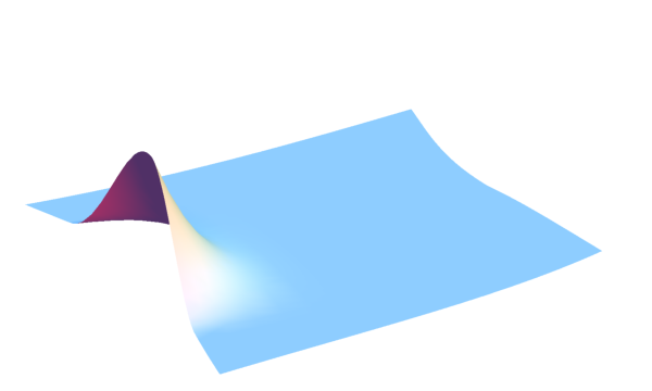
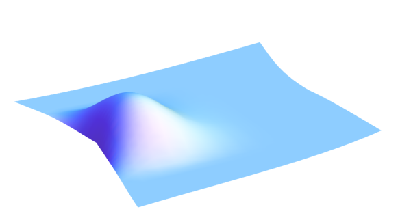
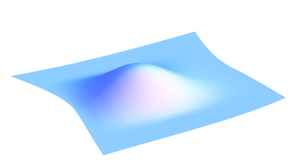
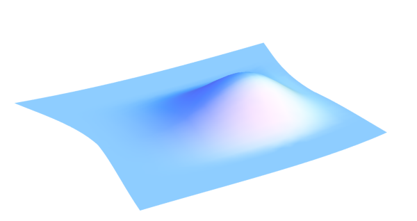
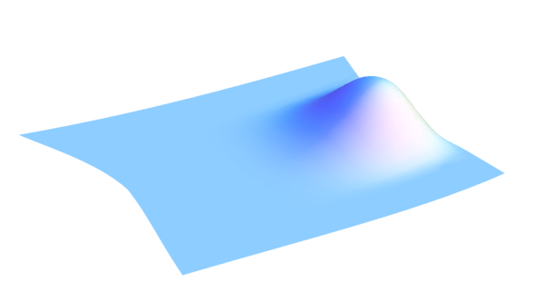
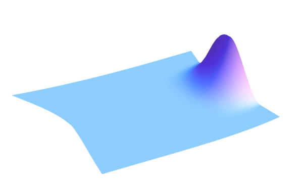
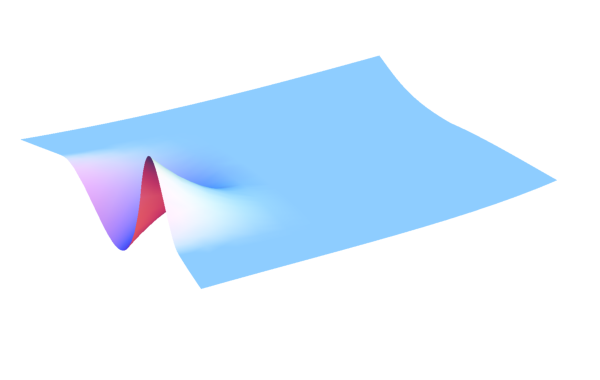
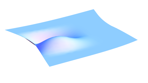
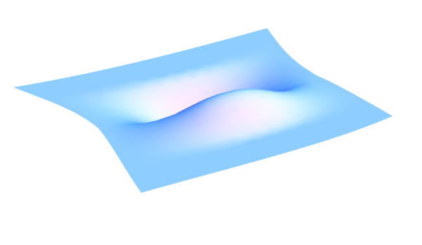
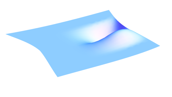
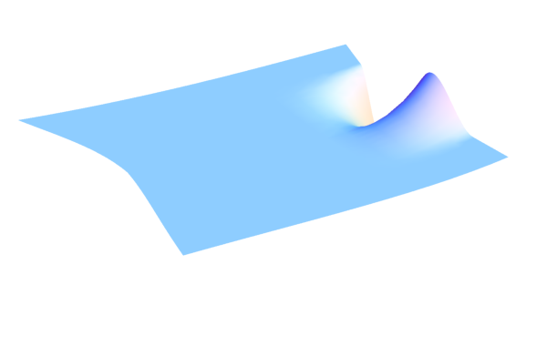
Fig. 1 shows the graphs of the resulting basis functions ϕ0,i\phi_{0,i} and ϕ1,j\phi_{1,j} of the space 𝒱21\mathcal{V}^{1}_{2} for k=2k=2.

Refer to caption Refer to caption Refer to caption
AS G1G^{1} two-patch geometry ϕ0,0\phi_{0,0} ϕ0,1\phi_{0,1}
Refer to caption Refer to caption Refer to caption
ϕ0,2\phi_{0,2} ϕ0,3\phi_{0,3} ϕ0,4\phi_{0,4}
Refer to caption Refer to caption Refer to caption
ϕ0,5\phi_{0,5} ϕ1,0\phi_{1,0} ϕ1,1\phi_{1,1}
Refer to caption Refer to caption Refer to caption
ϕ1,2\phi_{1,2} ϕ1,3\phi_{1,3} ϕ1,4\phi_{1,4}
Figure 1: The graphs of the basis functions ϕ0,i\phi_{0,i} and ϕ1,j\phi_{1,j} of the resulting space 𝒱21\mathcal{V}^{1}_{2} for the given bicubic AS G1G^{1} two-patch geometry, when both patches 𝑭(L)\boldsymbol{F}^{(L)} and 𝑭(R)\boldsymbol{F}^{(R)} are represented in the space 𝒮⁡(𝒯k3,1,[0,1]2)\mathcal{S}(\mathcal{T}^{3,1}_{k},[0,1]^{2}) for k=2k=2. (The graphs are plotted in the parameter range [0,12]×[0,1][0,\frac{1}{2}]\times[0,1] for both patches 𝑭(L)\boldsymbol{F}^{(L)} and 𝑭(R)\boldsymbol{F}^{(R)}.)

Let ϕi\phi_{i}, i=0,…,22+26​k+8​k2i=0,\ldots,22+26k+8k^{2}, be the C1C^{1}-smooth isogeometric basis functions of 𝒱1\mathcal{V}^{1}, which are collected as follows:

ϕi={ϕ⌊i/(4+2​k)⌋+2,imod(4+2​k)(L) if ​0≤i≤7+12​k+4​k2ϕ⌊(i−8−12​k−4​k2)/(4+2​k)⌋+2,imod(4+2​k)(R) if ​8+12​k+4​k2≤i≤15+24​k+8​k2ϕ0,i−16−24​k−8​k2 if ​16+24​k+8​k2≤i≤19+25​k+8​k2,ϕ1,i−20−25​k−8​k2 if ​20+25​k+8​k2≤i≤22+26​k+8​k2.\phi_{i}=\left\{\begin{array}[]{cl}\phi^{(L)}_{\lfloor i/(4+2k)\rfloor+2,i\bmod(4+2k)}&\mbox{ if }0\leq i\leq 7+12k+4k^{2}\\ \phi^{(R)}_{\lfloor(i-8-12k-4k^{2})/(4+2k)\rfloor+2,i\bmod(4+2k)}&\mbox{ if }8+12k+4k^{2}\leq i\leq 15+24k+8k^{2}\\ \phi_{0,i-16-24k-8k^{2}}&\mbox{ if }16+24k+8k^{2}\leq i\leq 19+25k+8k^{2},\\ \phi_{1,i-20-25k-8k^{2}}&\mbox{ if }20+25k+8k^{2}\leq i\leq 22+26k+8k^{2}.\end{array}\right.

In addition, we denote by gi(S)g^{(S)}_{i}, S∈{L,R}S\in\{L,R\}, the associated spline functions ϕi∘𝑭(S)\phi_{i}\circ\boldsymbol{F}^{(S)}. Let us consider the mass matrix M=(mi,j)i,j∈{0,…,22+26​k+8​k2}M=(m_{i,j})_{i,j\in\{0,\ldots,22+26k+8k^{2}\}} with the entries

mi,j=∫Ωϕi​(𝒙)​ϕj​(𝒙)​𝑑𝒙=∑S∈{L,R}∫01∫01gi(S)​(u,v)​gj(S)​(u,v)​|det(J(S)​(u,v))|​𝑑u​𝑑v,m_{i,j}=\int_{\Omega}\phi_{i}(\boldsymbol{x})\phi_{j}(\boldsymbol{x})\mathrm{d}\boldsymbol{x}=\sum_{S\in\{L,R\}}\int_{0}^{1}\int_{0}^{1}g^{(S)}_{i}(u,v)g^{(S)}_{j}(u,v)|\det(J^{(S)}(u,v))|\mathrm{d}u\mathrm{d}v,

where J(S)J^{(S)}, S∈{L,R}S\in\{L,R\}, is the Jacobian of 𝑭(S)\boldsymbol{F}^{(S)}. We also compute (for comparison) the mass matrix for the standard C0C^{0}-smooth isogeometric basis functions of the space 𝒱0=𝒱∩C0​(Ω)\mathcal{V}^{0}=\mathcal{V}\cap C^{0}(\Omega). Table 1 reports for different kk the condition numbers κ\kappa of the diagonally scaled mass matrices MM (cf. [7]) for the two different bases. The results indicate that the basis functions ϕi\phi_{i} are as well conditioned as the standard C0C^{0}-smooth isogeometric basis functions.

kk 0 1 2 3 4 5 10 15 20 30 40
𝒱0\mathcal{V}^{0} 938.91 724.57 654.29 624.71 608.64 598.63 578.41 572.41 569.93 567.89 567.31
𝒱1\mathcal{V}^{1} 273.49 425.71 520.62 552.6 564.4 569.07 571.02 569.51 568.51 567.58 567.28
Table 1: For different kk, the condition numbers κ\kappa of the diagonally scaled mass matrices MM for the standard C0C^{0}-smooth isogeometric basis functions (𝒱0\mathcal{V}^{0}) and our C1C^{1}-smooth isogeometric basis functions (𝒱1\mathcal{V}^{1}), cf. Example 15.

6 Spline coefficients of the basis functions of the space 𝒱21\mathcal{V}^{1}_{2}

We represent the spline functions g(S)=ϕ∘𝑭(S)g^{(S)}=\phi\circ\boldsymbol{F}^{(S)}, S∈{L,R}S\in\{L,R\}, for the previous constructed isogeometric basis functions ϕ\phi of the space 𝒱21\mathcal{V}^{1}_{2} as a linear combination of the tensor-product B-splines Ni,jp,rN_{i,j}^{p,r}. Thereby, these linear factors (i.e. the B-spline coefficients of the spline functions g(S)g^{(S)} with respect to the space 𝒮⁡(𝒯kp,r,[0,1]2)\mathcal{S}(\mathcal{T}^{p,r}_{k},[0,1]^{2})) will be described by means of blossoming. For the sake of simplicity (especially with respect to notation), we will restrict ourselves below to the case β=0{\beta}=0 or zβ=0z_{\beta}=0. Note that our framework could be also extended to the remaining cases.

6.1 Concept of blossoming

We give a short overview of the concept of blossoming. For more detail we refer to e.g. [8, 11, 21, 29, 30]. Given a univariate spline function h∈𝒮⁡(𝒯kp,r)h\in\mathcal{S}(\mathcal{T}^{p,r}_{k}) with the spline representation (1), there exists a uniquely defined function H:ℝp→ℝH:\mathbb{R}^{p}\rightarrow\mathbb{R}, called the blossom of hh, possessing the following properties:

  • 1.

    HH is symmetric,

  • 2.

    HH is multi-affine, and

  • 3.

    H⁡(t,…,t)=h⁡(t)H(t,\ldots,t)=h(t).

These properties imply (by the so called dual function property, see [11])

H(ti+1p,r,…,ti+pp,r)=di, i=0,…,p+k(p−r),H(t^{p,r}_{i+1},\ldots,t^{p,r}_{i+p})=d_{i},\mbox{ }i=0,\ldots,p+k(p-r),

and therefore fully determine the blossom, since the value H⁡(s1,…,sp)H(s_{1},\ldots,s_{p}) for arbitrary values s1,…,sps_{1},\ldots,s_{p} can be computed by recursively using the convex combinations

H⁡(ti+1p,r,…,ti+p−mp,r,s1,…,sm)=\displaystyle H(t^{p,r}_{i+1},\ldots,t^{p,r}_{i+p-m},s_{1},\ldots,s_{m})=
(1−γim​(sm))​H​(tip,r,…,ti+p−mp,r,s1,…,sm−1)+γim​(sm)​H​(ti+1p,r,…,ti+p−m+1p,r,s1,…,sm−1),\displaystyle(1-\gamma_{i}^{m}(s_{m}))H(t^{p,r}_{i},\ldots,t^{p,r}_{i+p-m},s_{1},\ldots,s_{m-1})+\gamma_{i}^{m}(s_{m})H(t^{p,r}_{i+1},\ldots,t^{p,r}_{i+p-m+1},s_{1},\ldots,s_{m-1}),

for i=m,…,p+k​p−ri=m,\ldots,p+k{p-r}, m=1,…,pm=1,\ldots,p and

γim​(s)=s−tip,rti+p−m+1p,r−tip,r.\gamma_{i}^{m}(s)=\frac{s-t^{p,r}_{i}}{t^{p,r}_{i+p-m+1}-t^{p,r}_{i}}.

The concept of blossoming provides a simple way to perform knot insertion, to differentiate a spline function and to multiply two spline functions. Given the spline function h∈𝒮⁡(𝒯kp,r,[0,1])h\in\mathcal{S}(\mathcal{T}^{p,r}_{k},[0,1]) with the blossom HH. Representing hh as a spline function in the space 𝒮⁡(𝒯kp,r−1,[0,1])\mathcal{S}(\mathcal{T}^{p,r-1}_{k},[0,1]), the corresponding spline control points d¯i\bar{d}_{i} are given by

d¯i=H(ti+1p,r−1,…,ti+pp,r−1),i=0,…,p+k(p−r+1).\bar{d}_{i}=H(t^{p,r-1}_{i+1},\ldots,t^{p,r-1}_{i+p}),\quad i=0,\ldots,p+k(p-r+1).

The spline control points d~i\tilde{d}_{i} of the derivative of hh, i.e. h′∈𝒮⁡(𝒯kp−1,r−1,[0,1])h^{\prime}\in\mathcal{S}(\mathcal{T}^{p-1,r-1}_{k},[0,1]), can be computed as follows:

d~i=pti+p+1p,r−ti+1p,r​(H⁡(ti+1p−1,r−1,…,ti+p−1p−1,r−1,ti+p+1p,r)−H⁡(ti+1p−1,r−1,…,ti+p−1p−1,r−1,ti+1p,r))\tilde{d}_{i}=\frac{p}{t_{i+p+1}^{p,r}-t_{i+1}^{p,r}}(H(t_{i+1}^{p-1,r-1},\ldots,t_{i+p-1}^{p-1,r-1},t_{i+p+1}^{p,r})-H(t_{i+1}^{p-1,r-1},\ldots,t_{i+p-1}^{p-1,r-1},t_{i+1}^{p,r}))

for i=0,…,p−1+k⁡(p−r)i=0,\ldots,p-1+k(p-r). Given further the spline function h1∈𝒮⁡(𝒯kp1,r1,[0,1])h_{1}\in\mathcal{S}(\mathcal{T}^{p_{1},r_{1}}_{k},[0,1]) with the blossom H1H_{1}. Let p^=p+p1\hat{p}=p+p_{1} and r^=min⁡(r,r1)\hat{r}=\min(r,r_{1}). Then the spline control points d^i\hat{d}_{i} of the product h^=h​h1∈𝒮⁡(𝒯kp^,r^,[0,1])\hat{h}=hh_{1}\in\mathcal{S}(\mathcal{T}^{\hat{p},\hat{r}}_{k},[0,1]) are given by

d^i=1(p^p)∑H(ti1p^,r^,…,tipp^,r^)H1(tip+1p^,r^,…,tip^p^,r^),i=0,…,p^+k(p^−r^),\hat{d}_{i}=\frac{1}{{\hat{p}\choose p}}\sum H(t_{i_{1}}^{\hat{p},\hat{r}},\ldots,t_{i_{p}}^{\hat{p},\hat{r}})H_{1}(t_{i_{p+1}}^{\hat{p},\hat{r}},\ldots,t_{i_{\hat{p}}}^{\hat{p},\hat{r}}),\quad i=0,\ldots,\hat{p}+k(\hat{p}-\hat{r}),

where the summation runs over all possibilities to split the set {i+1,…,i+p^}\{i+1,\ldots,i+\hat{p}\} into the two disjoint subsets {i1,…,ip}\{i_{1},\ldots,i_{p}\} and {ip+1,…,ip^}\{i_{p+1},\ldots,i_{\hat{p}}\}.

6.2 Spline coefficients as matrix entries

Let n=p+1+k⁡(p−r)n=p+1+k(p-r), n~=p+1+k⁡(p−r−1)+zβ\tilde{n}=p+1+k(p-r-1)+z_{\beta} and n¯=p+1−dα+k⁡(p+1−dα−r)\bar{n}=p+1-d_{\alpha}+k(p+1-d_{\alpha}-r). We denote by g0,i(S)g_{0,i}^{(S)}, i=0,…,n~−1i=0,\ldots,\tilde{n}-1, and g1,j(S)g_{1,j}^{(S)}, j=0,…,n¯−1j=0,\ldots,\bar{n}-1, for S∈{L,R}S\in\{L,R\} the spline functions ϕ0,i∘𝑭(S)\phi_{0,i}\circ\boldsymbol{F}^{(S)}, and ϕ1,j∘𝑭(S)\phi_{1,j}\circ\boldsymbol{F}^{(S)}, respectively. In addition, let 𝑩(S)=(𝑩0(S),𝑩1(S))T\boldsymbol{B}^{(S)}=(\boldsymbol{B}^{(S)}_{0},\boldsymbol{B}^{(S)}_{1})^{T} be the vector of functions, where

𝑩0(S)​(u,v)=(g0,0(S)​(u,v),…,g0,n~−1(S)​(u,v))T,\boldsymbol{B}^{(S)}_{0}(u,v)=(g_{0,0}^{(S)}(u,v),\ldots,g_{0,\tilde{n}-1}^{(S)}(u,v))^{T},

as well as

𝑩1(S)​(u,v)=(g1,0(S)​(u,v),…,g1,n¯−1(S)​(u,v))T,\boldsymbol{B}^{(S)}_{1}(u,v)=(g_{1,0}^{(S)}(u,v),\ldots,g_{1,\bar{n}-1}^{(S)}(u,v))^{T},

and let 𝑩∗=(𝑩0∗,𝑩1∗)T\boldsymbol{B}^{*}=(\boldsymbol{B}^{*}_{0},\boldsymbol{B}^{*}_{1})^{T} be the vector of functions, where

𝑩0∗​(u,v)=(N0,0p,r​(u,v),…,N0,n−1p,r​(u,v))T,\boldsymbol{B}^{*}_{0}(u,v)=(N_{0,0}^{p,r}(u,v),\ldots,N_{0,n-1}^{p,r}(u,v))^{T},

as well as

𝑩1∗​(u,v)=(N1,0p,r​(u,v),…,N1,n−1p,r​(u,v))T.\boldsymbol{B}^{*}_{1}(u,v)=(N_{1,0}^{p,r}(u,v),\ldots,N_{1,n-1}^{p,r}(u,v))^{T}.

Then there exists a matrix A(S)∈ℝ(n~+n¯)×2​nA^{(S)}\in\mathbb{R}^{(\tilde{n}+\bar{n})\times 2n} such that

𝑩(S)​(u,v)=A(S)​𝑩∗​(u,v).\boldsymbol{B}^{(S)}(u,v)=A^{(S)}\boldsymbol{B}^{*}(u,v).

The matrix A(S)A^{(S)} for S∈{L,R}S\in\{L,R\} has a block structure, resulting in an equation of the form

(𝑩0(S)𝑩1(S))=(A1A2(S)0A3(S))​(𝑩0∗𝑩1∗),\left(\begin{array}[]{c}\boldsymbol{B}^{(S)}_{0}\\ \boldsymbol{B}^{(S)}_{1}\end{array}\right)=\left(\begin{array}[]{cc}A_{1}&A_{2}^{(S)}\\ 0&A_{3}^{(S)}\end{array}\right)\left(\begin{array}[]{c}\boldsymbol{B}^{*}_{0}\\ \boldsymbol{B}^{*}_{1}\end{array}\right), (25)

where A1∈ℝn~×nA_{1}\in\mathbb{R}^{\tilde{n}\times n}, A2(S)∈ℝn~×nA_{2}^{(S)}\in\mathbb{R}^{\tilde{n}\times n} and A3(S)∈ℝn¯×nA_{3}^{(S)}\in\mathbb{R}^{\bar{n}\times n}. For each row the single entries of the matrix A(S)A^{(S)}, S∈{L,R}S\in\{L,R\}, provide the B-spline coefficients of the corresponding spline function g0,i(S)g_{0,i}^{(S)} or g1,j(S)g_{1,j}^{(S)} with respect to the spline space 𝒮⁡(𝒯kp,r,[0,1]2)\mathcal{S}(\mathcal{T}^{p,r}_{k},[0,1]^{2}).

The following lemma provides the entries of the single matrices A1A_{1}, A2(S)A_{2}^{(S)} and A3(S)A_{3}^{(S)}:

Lemma 16.

We denote by Hip,rH_{i}^{p,r} the blossom of the B-spline Nip,rN_{i}^{p,r}. For a linear function w:[0,1]→ℝw:[0,1]\rightarrow\mathbb{R} with the Bézier representation

w(t)=w0(1−t)+w1t,t∈[0,1],w0,w1∈ℝ,w(t)=w_{0}(1-t)+w_{1}t,\quad t\in[0,1],\quad w_{0},w_{1}\in\mathbb{R}, (26)

we define the matrix A^​(w)=(a^i,j(w))i,j\hat{A}{(w)}=(\hat{a}^{(w)}_{i,j})_{i,j} given by

a^i,j(w)=1p​∑l=1p((1−tlp,r)​w0+tlp,r​w1)​Hip−1,r​(tj+1p,r,…,tl−1p,r,tl+1p,r,…,tj+pp,r).\hat{a}^{(w)}_{i,j}=\frac{1}{p}\sum_{l=1}^{p}((1-t_{l}^{p,r})w_{0}+t_{l}^{p,r}w_{1})H_{i}^{p-1,r}(t_{j+1}^{p,r},\ldots,t_{l-1}^{p,r},t_{l+1}^{p,r},\ldots,t_{j+p}^{p,r}).

The matrices A1A_{1}, A2(S)A_{2}^{(S)} and A3(S)A_{3}^{(S)}, compare (25), are given as follows (depending on α(S)\alpha^{(S)}, β(S)\beta^{(S)} or β\beta):

  • 1.

    Let β=0\beta=0. Then we have

    A1=A2(S)=In, and ​A3(S)={1(k+1)​p​α(S)​In if ​dα=0,1(k+1)​p​A^​(α(S)) if ​dα=1.A_{1}=A^{(S)}_{2}=I_{n},\mbox{ and }A^{(S)}_{3}=\left\{\begin{array}[]{cl}\frac{1}{(k+1)p}\alpha^{(S)}I_{n}&\mbox{ if }d_{\alpha}=0,\\ \frac{1}{(k+1)p}\hat{A}{(\alpha^{(S)})}&\mbox{ if }d_{\alpha}=1.\end{array}\right.
  • 2.

    Let zβ=0z_{\beta}=0. Then we have

    A1=A¯, A2(S)=A¯+1(k+1)​pA~A^(β(S)), and A3(S)={1(k+1)​p​α(S)​In if ​dα=0,1(k+1)​p​A^​(α(S)) if ​dα=1,A_{1}=\bar{A},\mbox{ }A^{(S)}_{2}=\bar{A}+\frac{1}{(k+1)p}\tilde{A}\hat{A}{(\beta^{(S)})},\mbox{ and }A^{(S)}_{3}=\left\{\begin{array}[]{cl}\frac{1}{(k+1)p}\alpha^{(S)}I_{n}&\mbox{ if }d_{\alpha}=0,\\ \frac{1}{(k+1)p}\hat{A}{(\alpha^{(S)})}&\mbox{ if }d_{\alpha}=1,\end{array}\right.

    where the entries of the matrices A¯=(a¯i,j)i,j\bar{A}=(\bar{a}_{i,j})_{i,j} and A~=(a~i,j)i,j\tilde{A}=(\tilde{a}_{i,j})_{i,j} are given by

    a¯i,j=Hip,r+1​(tj+1p,r,…,tj+pp,r)\bar{a}_{i,j}=H_{i}^{p,r+1}(t_{j+1}^{p,r},\ldots,t_{j+p}^{p,r})

    and

    a~i,j=ptj+p+1p,r+1−tj+1p,r+1​(Hip,r+1​(tj+1p−1,r,…,tj+p−1p−1,r,tj+p+1p,r+1)−Hip,r+1​(tj+1p−1,r,…,tj+p−1p−1,r,tj+1p,r+1)),\tilde{a}_{i,j}=\frac{p}{t_{j+p+1}^{p,r+1}-t_{j+1}^{p,r+1}}(H_{i}^{p,r+1}(t_{j+1}^{p-1,r},\ldots,t_{j+p-1}^{p-1,r},t_{j+p+1}^{p,r+1})-H_{i}^{p,r+1}(t_{j+1}^{p-1,r},\ldots,t_{j+p-1}^{p-1,r},t_{j+1}^{p,r+1})),

    respectively.

Here, InI_{n} is the identity matrix of dimension nn.

Proof.

The results follow directly from the concept of blossoming as presented in Subsection 6.1. ∎

Remark 17.

The matrices A1A_{1}, A2(S)A_{2}^{(S)} and A3(S)A_{3}^{(S)}, see (25), are sparse matrices (compare Example 19).

Remark 18.

A further possibility to construct the matrices A1A_{1}, A2(S)A_{2}^{(S)} and A3(S)A_{3}^{(S)}, see (25), is the use of the concept of fitting. Thereby, the mm-th row of the matrices A1A_{1}, A2(S)A_{2}^{(S)} and A3(S)A_{3}^{(S)}, denoted by (a1,m,0,…,a1,m,n−1)(a_{1,m,0},\ldots,a_{1,m,n-1}), (a2,m,0(S),…,a2,m,n−1(S))(a^{(S)}_{2,m,0},\ldots,a^{(S)}_{2,m,n-1}) and (a3,m,0(S),…,a3,m,n−1(S))(a^{(S)}_{3,m,0},\ldots,a^{(S)}_{3,m,n-1}), respectively, are computed by minimizing the terms

∑i=0n−1(g0,m(L)​(0,ξi)−∑jn−1a1,m,j​Njp,r​(ξi))2,\sum_{i=0}^{n-1}(g^{(L)}_{0,m}(0,\xi_{i})-\sum_{j}^{n-1}a_{1,m,j}N_{j}^{p,r}(\xi_{i}))^{2},
∑i=0n−1(Du​g0,m(S)​(0,ξi)p+g0,m(S)​(0,ξi)−∑jn−1a2,m,j(S)​Njp,r​(ξi))2\sum_{i=0}^{n-1}(\frac{D_{u}g^{(S)}_{0,m}(0,\xi_{i})}{p}+g^{(S)}_{0,m}(0,\xi_{i})-\sum_{j}^{n-1}a^{(S)}_{2,m,j}N_{j}^{p,r}(\xi_{i}))^{2}

and

∑i=0n−1(Du​g1,m(S)​(0,ξi)p+g1,m(S)​(0,ξi)−∑jn−1a3,m,j(S)​Njp,r​(ξi))2,\sum_{i=0}^{n-1}(\frac{D_{u}g^{(S)}_{1,m}(0,\xi_{i})}{p}+g^{(S)}_{1,m}(0,\xi_{i})-\sum_{j}^{n-1}a^{(S)}_{3,m,j}N_{j}^{p,r}(\xi_{i}))^{2},

respectively, where (ξi)i=0,…,n−1(\xi_{i})_{i=0,\ldots,n-1} are the Greville abscissa of the B-splines Njp,rN_{j}^{p,r}, j=0,…,n−1j=0,\ldots,n-1, of the spline space 𝒮⁡(𝒯kp,r,[0,1])\mathcal{S}(\mathcal{T}_{k}^{p,r},[0,1]).

Example 19.

Let β≠0{\beta}\neq 0 and zβ=0z_{\beta}=0, p=3p=3, r=1r=1, k≥2k\geq 2 and τi=ik+1\tau_{i}=\frac{i}{k+1} for i=1,…,ki=1,\ldots,k. Let w:[0,1]→ℝw:[0,1]\rightarrow\mathbb{R} be a linear function with the Bézier representation (26). Then the rows a¯i\bar{a}_{i}, a~i\tilde{a}_{i} and a^i(w)\hat{a}_{i}^{(w)} of the matrices A¯\bar{A}, A~\tilde{A} and A^​(w)\hat{A}(w) from Lemma 16 are given as follows:

a¯i={(1,0,…,0⏟2​k+3)​i=0(0,1,12,0,…,0⏟2​k+1)​i=1(0,0,12,23,13,0,…,0⏟2​k−1)​i=2(0,…,0⏟2​i−3,13,23,23,13,0,…,0⏟2​(k−i)+3)​3≤i≤k(0,…,0⏟2​k−1,13,23,12,0,0)​i=k+1(0,…,0⏟2​k+1,12,1,0)​i=k+2(0,…,0⏟2​k+3,1)​i=k+3​, ​a~i={(−3​(k+1),0,…,0⏟k+2)​i=0(3​(k+1),−3​(k+1)2,0,…,0⏟k+1)​i=1(0,3​(k+1)2,−(k+1),0,…,0⏟k)​i=2(0,…,0⏟i−1,k+1,−(k+1),0,…,0⏟k−i+2)​3≤i≤k(0,…,0⏟k,k+1,−3​(k+1)2,0)​i=k+1(0,…,0⏟k+1,3​(k+1)2,−3​(k+1))​i=k+2(0,…,0⏟k+2,3​(k+1))​i=k+3\bar{a}_{i}=\begin{cases}(1,\underbrace{0,\ldots,0}_{2k+3})\hskip 8.19447pti=0\\ (0,1,\frac{1}{2},\underbrace{0,\ldots,0}_{2k+1})\hskip 8.19447pti=1\\ (0,0,\frac{1}{2},\frac{2}{3},\frac{1}{3},\underbrace{0,\ldots,0}_{2k-1})\hskip 8.19447pti=2\\ (\underbrace{0,\ldots,0}_{2i-3},\frac{1}{3},\frac{2}{3},\frac{2}{3},\frac{1}{3},\underbrace{0,\ldots,0}_{2(k-i)+3})\hskip 8.19447pt3\leq i\leq k\\ (\underbrace{0,\ldots,0}_{2k-1},\frac{1}{3},\frac{2}{3},\frac{1}{2},0,0)\hskip 8.19447pti=k+1\\ (\underbrace{0,\ldots,0}_{2k+1},\frac{1}{2},1,0)\hskip 8.19447pti=k+2\\ (\underbrace{0,\ldots,0}_{2k+3},1)\hskip 8.19447pti=k+3\end{cases}\mbox{, }\tilde{a}_{i}=\begin{cases}(-3(k+1),\underbrace{0,\ldots,0}_{k+2})\hskip 8.19447pti=0\\ (3(k+1),-\frac{3(k+1)}{2},\underbrace{0,\ldots,0}_{k+1})\hskip 8.19447pti=1\\ (0,\frac{3(k+1)}{2},-(k+1),\underbrace{0,\ldots,0}_{k})\hskip 8.19447pti=2\\ (\underbrace{0,\ldots,0}_{i-1},k+1,-(k+1),\underbrace{0,\ldots,0}_{k-i+2})\hskip 8.19447pt3\leq i\leq k\\ (\underbrace{0,\ldots,0}_{k},k+1,-\frac{3(k+1)}{2},0)\hskip 8.19447pti=k+1\\ (\underbrace{0,\ldots,0}_{k+1},\frac{3(k+1)}{2},-3(k+1))\hskip 8.19447pti=k+2\\ (\underbrace{0,\ldots,0}_{k+2},3(k+1))\hskip 8.19447pti=k+3\end{cases}

and

a^i(w)=16​(k+1)∗{(6​(k+1)​w0,2​k​w0+2​w1,0,…,0⏟2​k+2)​i=0(0,4​(k+1)​w0,(1+5​k)​w0+4​w1,(k−1)​w0+2​w1,0,…,0⏟2​k)​i=1{(0,…,0⏟2​(i−1),(k+3−i)w0+(i−2)w1,(9+5(k−i))w0+(6+5(i−2))w1,OPEN(6+5​(k−i))​w0+(9+5​(i−2))​w1,(k−i)​w0+(i+1)​w1,0,…,0⏟2​(k−i+1))}​2≤i≤k(0,…,0⏟2​k,2​w0+(k−1)​w1,4​w0+(1+5​k)​w1,4​(k+1)​w1,0)​i=k+1(0,…,0⏟2​k+2,2​w0+2​k​w1,6​(k+1)​w1)​i=k+2\hat{a}^{(w)}_{i}=\frac{1}{6(k+1)}*\begin{cases}(6(k+1)w_{0},2kw_{0}+2w_{1},\underbrace{0,\ldots,0}_{2k+2})\hskip 8.19447pti=0\\ (0,4(k+1)w_{0},(1+5k)w_{0}+4w_{1},(k-1)w_{0}+2w_{1},\underbrace{0,\ldots,0}_{2k})\hskip 8.19447pti=1\\ \left\{\begin{array}[]{l}(\underbrace{0,\ldots,0}_{2(i-1)},(k+3-i)w_{0}+(i-2)w_{1},(9+5(k-i))w_{0}+(6+5(i-2))w_{1},\\ (6+5(k-i))w_{0}+(9+5(i-2))w_{1},(k-i)w_{0}+(i+1)w_{1},\underbrace{0,\ldots,0}_{2(k-i+1)})\end{array}\right\}\hskip 8.19447pt2\leq i\leq k\\ (\underbrace{0,\ldots,0}_{2k},2w_{0}+(k-1)w_{1},4w_{0}+(1+5k)w_{1},4(k+1)w_{1},0)\hskip 8.19447pti=k+1\\ (\underbrace{0,\ldots,0}_{2k+2},2w_{0}+2kw_{1},6(k+1)w_{1})\hskip 8.19447pti=k+2\end{cases}

7 Conclusion

We have studied the spaces of C1C^{1}-smooth isogeometric functions over a special class of two-patch geometries, so-called analysis-suitable G1G^{1} (AS G1G^{1}) two-patch parameterizations (cf. [9]). This class of two-patch geometries is of particular interest, since exactly these geometries allow under certain assumptions C1C^{1} isogeometric spaces with optimal approximation properties, see [9]. More precisely, we have computed the dimension of these C1C^{1} spaces and have presented an explicit basis construction. The resulting basis functions are well conditioned, have small local supports and their spline coefficients can be simply computed by means of blossoming or fitting.

Note that the constructed basis interpolates traces and transversal derivatives at the interface. Hence, the basis functions may be negative. In fact, the functions interpolating the transversal derivative are by construction positive on one side of the interface and negative on the other. The presented basis can be transformed easily to obtain locally supported basis functions which sum up to one. However, it is unclear whether or not a non-negative, local partition of unity exists for all AS G1G^{1} parameterizations. This will be of interest for future research.

One issue that remains to be studied is the flexibility of AS G1G^{1} geometries over general multi-patch domains. The basis construction over two-patch geometries can be applied also to multi-patch configurations except for the basis functions around vertices, where modifications might be necessary. We are confident that the presented basis representation can be extended to the multi-patch case and used for fitting procedures, that approximate any given geometry with an AS G1G^{1} parameterization.

The developed basis provides a simple representation that can be implemented in existing IGA libraries. Thus, our C1C^{1}-smooth functions may be used to discretize different fourth-order partial differential equations. It may be of interest for future studies to perform such simulations and analyze their properties as well as to investigate the class of AS G1G^{1} parameterizations for volumetric two-patch and multi-patch domains.

Acknowledgment

The authors wish to thank the anonymous reviewers for their comments that helped to improve the paper. The first two authors (M. Kapl and G. Sangalli) were partially supported by the European Research Council through the FP7 ERC Consolidator Grant n.616563 HIGEOM, and by the Italian MIUR through the PRIN “Metodologie innovative nella modellistica differenziale numerica”. This support is gratefully acknowledged.

References

  • [1] F. Auricchio, L. Beirão da Veiga, A. Buffa, C. Lovadina, A. Reali, and G. Sangalli. A fully "locking-free" isogeometric approach for plane linear elasticity problems: a stream function formulation. Computer methods in applied mechanics and engineering, 197(1):160–172, 2007.
  • [2] A. Bartezzaghi, L. Dedè, and A. Quarteroni. Isogeometric analysis of high order partial differential equations on surfaces. Computer Methods in Applied Mechanics and Engineering, 295:446 – 469, 2015.
  • [3] L. Beirão da Veiga, A. Buffa, G. Sangalli, and R. Vázquez. Mathematical analysis of variational isogeometric methods. Acta Numerica, 23:157–287, 5 2014.
  • [4] L. Beirao da Veiga, A. Buffa, C. Lovadina, M. Martinelli, and G. Sangalli. An isogeometric method for the Reissner–Mindlin plate bending problem. Computer Methods in Applied Mechanics and Engineering, 209:45–53, 2012.
  • [5] D. J. Benson, Y. Bazilevs, M.-C. Hsu, and T. J.R. Hughes. A large deformation, rotation-free, isogeometric shell. Computer Methods in Applied Mechanics and Engineering, 200(13):1367–1378, 2011.
  • [6] M. Bercovier and T. Matskewich. Smooth Bézier surfaces over arbitrary quadrilateral meshes. Technical Report 1412.1125, arXiv.org, 2014.
  • [7] A. M. Bruaset. A survey of preconditioned iterative methods, volume 328 of Pitman Research Notes in Mathematics Series. Longman Scientific & Technical, Harlow, 1995.
  • [8] X. Chen, R. F. Riesenfeld, and E. Cohen. An algorithm for direct B-spline multiplication. IEEE Transactions on Automation Science and Engineering, 6(3):433 – 442, 2009.
  • [9] A. Collin, G. Sangalli, and T. Takacs. Analysis-suitable G1 multi-patch parametrizations for C1 isogeometric spaces. Computer Aided Geometric Design, 47:93 – 113, 2016.
  • [10] J. A. Cottrell, T.J.R. Hughes, and Y. Bazilevs. Isogeometric Analysis: Toward Integration of CAD and FEA. John Wiley & Sons, Chichester, England, 2009.
  • [11] R. Goldman. Pyramid algorithms : a dynamic programming approach to curves and surfaces for geometric modeling. Morgan Kaufmann, San Francisco (Calif.), 2003.
  • [12] H. Gómez, V. M Calo, Y. Bazilevs, and T. J.R. Hughes. Isogeometric analysis of the Cahn–Hilliard phase-field model. Computer Methods in Applied Mechanics and Engineering, 197(49):4333–4352, 2008.
  • [13] H. Gómez, T. J.R. Hughes, X. Nogueira, and V. M. Calo. Isogeometric analysis of the isothermal Navier–Stokes–Korteweg equations. Computer Methods in Applied Mechanics and Engineering, 199(25):1828–1840, 2010.
  • [14] J. Hoschek and D. Lasser. Fundamentals of computer aided geometric design. A K Peters Ltd., Wellesley, MA, 1993.
  • [15] T. J. R. Hughes, J. A. Cottrell, and Y. Bazilevs. Isogeometric analysis: CAD, finite elements, NURBS, exact geometry and mesh refinement. Comput. Methods Appl. Mech. Engrg., 194(39-41):4135–4195, 2005.
  • [16] M. Kapl, F. Buchegger, M. Bercovier, and B. Jüttler. Isogeometric analysis with geometrically continuous functions on planar multi-patch geometries. Comput. Methods Appl. Mech. Engrg., pages –, 2016.
  • [17] M. Kapl, V. Vitrih, B. Jüttler, and K. Birner. Isogeometric analysis with geometrically continuous functions on two-patch geometries. Comput. Math. Appl., 70(7):1518 – 1538, 2015.
  • [18] K. Karčiauskas, T. Nguyen, and J. Peters. Generalizing bicubic splines for modeling and IGA with irregular layout. Computer-Aided Design, 70:23 – 35, 2016.
  • [19] J. Kiendl, Y. Bazilevs, M.-C. Hsu, R. Wüchner, and K.-U. Bletzinger. The bending strip method for isogeometric analysis of Kirchhoff-Love shell structures comprised of multiple patches. Computer Methods in Applied Mechanics and Engineering, 199(35):2403–2416, 2010.
  • [20] J. Kiendl, K.-U. Bletzinger, J. Linhard, and R. Wüchner. Isogeometric shell analysis with Kirchhoff-Love elements. Computer Methods in Applied Mechanics and Engineering, 198(49):3902–3914, 2009.
  • [21] W. Liu. A simple, efficient degree raising algorithm for B-spline curves. Computer Aided Geometric Design, 14(7):693 – 698, 1997.
  • [22] T. Matskewich. Construction of C1C^{1} surfaces by assembly of quadrilateral patches under arbitrary mesh topology. PhD thesis, Hebrew University of Jerusalem, 2001.
  • [23] B. Mourrain, R. Vidunas, and N. Villamizar. Dimension and bases for geometrically continuous splines on surfaces of arbitrary topology. Computer Aided Geometric Design, 45:108 – 133, 2016.
  • [24] T. Nguyen, K. Karčiauskas, and J. Peters. A comparative study of several classical, discrete differential and isogeometric methods for solving poisson’s equation on the disk. Axioms, 3(2):280–299, 2014.
  • [25] T. Nguyen, K. Karčiauskas, and J. Peters. C1{C}^{1} finite elements on non-tensor-product 2d and 3d manifolds. Applied Mathematics and Computation, 272:148 – 158, 2016.
  • [26] T. Nguyen and J. Peters. Refinable C1{C}^{1} spline elements for irregular quad layout. Computer Aided Geometric Design, 43:123 – 130, 2016.
  • [27] J. Peters. Smooth mesh interpolation with cubic patches. Computer-Aided Design, 22(2):109 – 120, 1990.
  • [28] J. Peters. Geometric continuity. In Handbook of computer aided geometric design, pages 193–227. North-Holland, Amsterdam, 2002.
  • [29] L. Ramshaw. Blossoms are polar forms. Comput. Aided Geom. Des., 6(4):323–358, 1989.
  • [30] H.-P. Seidel. An introduction to polar forms. IEEE Computer Graphics and Applications, 13(1):38–46, 1993.
  • [31] A. Tagliabue, L. Dedè, and A. Quarteroni. Isogeometric analysis and error estimates for high order partial differential equations in fluid dynamics. Computers & Fluids, 102:277 – 303, 2014.