Spatially-resolved measurements of micro-deformations in granular materials using Diffusing Wave Spectroscopy
Abstract
This article is a tutorial on the practical implementation of a method of measurement of minute deformations based on multiple scattering. This technique has been recently developed and has proven to give new insights on the spatial repartition of strain in a granular material. We provide here the basics to understand the method by giving a synthetic review on Diffusing Wave Spectroscopy and multiple scattering in granular materials. We detail a simple experiment using standard lab equipment to pedagogically demonstrate the implementation of the method. Finally we give a few examples of measurements that have been obtained in other works to discuss the potential of the method.
pacs
42.25.Dd, 42.30.Ms, 45.70.-nI Introduction
Numerous types of disordered media, as foams, grains or concentrate colloidals suspensions strongly scatter light because of their heterogeneities. This feature is usually considered as an obstacle to accurate optical diagnoses in those materials. However information can be extracted from the light multiply scattered by a sample, giving access to local minute relative displacements [1, 2]. The possibility of such measurements in strongly scattering media have raised a lot of interest for the study of soft glassy materials as those systems are often turbid. The earliest works devoted to Brownian motion in colloidal suspensions [3, 4] have been rapidly extended to other scattering media as foams [5, 6], emulsions [7] or granular materials [8]. For all those systems, measurements based on multiple scattering have proven to be crucial for the understanding of their dynamics [9]. A potential drawback of those methods is that intrinsically only mean quantities can be obtained as the underlying multiple scattering process produce a natural averaging of the information. Numerous works have been devoted to improvements and variations of the original method [10] in particular with the goal of characterizing non-ergodic and heterogeneous dynamics [11, 12, 13, 14, 15, 16]. Of particular interest here are the methods which allow to achieve spatial information [16, 17, 19]. Full-field methods of measurement of strain and displacement based on speckle interferometry has been developped since the 70’s [20, 21]. Those methods are based on the measurement of planar displacements and deformation of a rough surface. In the case of the method presented here, the light penetrates inside the material and the information collected is not merely surfacic [22].
In the present article we show in details the implementation of a method of measurement of tiny deformation based on multiple scattering. The method is based on the measurement of auto-correlation function of the light intensity multiply scattered by a strongly scattering material. We provide here the basics needed to understand the method and implement it practically in a lab.
Part II is an introduction to Diffusing Wave Spectroscopy (DWS) giving the essentials to understand the method. Part III covers the specific case of granular materials. Scattering processes in a granular assembly is discussed. The effect of correlated and uncorrelated motion of the scatterers on the phase shift is presented, leading to a general expression of the auto-correlation function of the scattered intensity as a function of the strain field. The principle of the method for obtaining a spatially resolved strain maps is then presented. Part IV is a tutorial describing in full details the implementation of the method in a simple experiment based on heat conduction in a granular material. It provides all practical details of the adjustments that have to be done to perform the experiment properly. The last part presents a short review of the literature of measurements that have been done on granular systems using the method and indicating its potential and limitations.
II DWS theory
II.1 General principle
In a strongly scattering material, light rays follow different paths, each path being composed of numerous scattering events (see Fig. 1). When the source is coherent, the light transmitted through or backscattered from a disorder system gives rise to constructive and destructive wave interference and the collected intensities display a speckle figure (see Fig. 1). The scattered light rays have performed a random walk inside the material and thus have explored a part of the bulk of the material.

If the system has an internal dynamics (e.g., Brownian motion for a colloidal suspension) the speckle figure will change with time. The principle of the Diffusing-Wave Spectroscopy (DWS) is to analyze the fluctuations of the scattered intensity in order to extract information about the structure or dynamics of the system [23, 1].
The principle of the analysis is based on the calculation of the auto-correlation function of the scattered intensities. The correlations are calculated between two states of the sample that we will call 1 and 2 in the following:
| (1) |
The average operation in Eq. (1) can be performed over time (it is then supposed that the phenomenon studied is ergodic), or over an ensemble of speckles [24]. In multi-speckles method [25], light intensity is collected on a CCD camera, each speckle being an independent representation of the same random process and an ensemble average is obtained by averaging over the pixels of the camera.

The loss of correlation measured between two speckle figures corresponds to two different states generated by the inner dynamics in the material (see Fig. 2). When single scattering is at play, information can be directly extracted when collecting the light at a given angle from the deviation of the wavevector. In the case of multiple scattering the wavevectors have experienced numerous deviations so that the dependence of the signal on the scattering angle is lost and no specific information can be inferred. Still, the modeling of the light propagating in the material as a diffusion process [27] makes it possible to characterize the dynamics in the system. Although the diffusion process causes the loss of most of the detailed information about the material in which it propagates, this process is also at the origin of the unmatched sensitivity of the method. Usually, the sensitivity of an interferometric method is of the order of the wavelength of the coherent source used. Indeed, a loss of correlation between two interferometric figures corresponds typically to the change from constructive interference to destructive one, i.e. to a change between the ray paths of the order of one wavelength. But as multiple scattering implies a large number of scattering events, decorrelation will occur when the scatterers will have move only of a fraction of the wavelength. Consequently, relative displacements of a few nanometers of the scatterers are measurable [1].
II.2 Amplitude and intensity correlation functions
Considering the field at a point on a sensor, its amplitude is the sum of a large number of rays . The correlation function of the amplitudes is:
| (2) |
which implies the cross term:
When averaging, the contribution from will vanish because the fields originating from different paths () can be considered as uncorrelated. Consequently:
with . This result means that the statistical properties of the fluctuations depend only on the phase variation of each paths. Consequently, understanding the form of the correlation function necessitates to calculate the typical phase variation of a path.
Experimentally the correlation is calculated over the intensities. When the scattered field has a Gaussian distribution, the correlation functions on amplitudes, , and the ones on intensities, , are linked by the Siegert relation [28]:
| (3) |
where is an experimental constant of order unity depending on the details of the experimental setup [28].
The function depends on the phase variation on each of path between the states 1 and 2. A variation of length of a path of length leads to a phase variation for the light ray following this path, with the wavevector of the light, and its wavelength. In the multiple scattering limit, each path is composed of numerous scattering events and the correlation function of the scattered field can be expressed as [1, 29]
| (4) |
where is the probability for an optical path to have the length . This distribution can be calculated from the diffusive equation knowing the boundary conditions of the experiment [27]. The quantity is the contribution of a path of length to the variation of the electric field between the states and and the average is done over all the paths of length .
All the information about the deformation or dynamics of the material is contained in the term [3]. The number of scattering events in each paths is large so that by the central limit theorem, is a random variable, and:
| (5) |
In the next section, the phase shift obtained for a deformed material will be detailed.
III Imaging granular materials
III.1 How scattering works in a granular material
The measured correlation functions of electromagnetic fields are related to the phase fluctuations according to eq. (4) in which the path length distribution needs to be known. This distribution is related to the transport of light into the granular material. Multiple light scattering during its propagation into the medium is characterized by two different lengths. First, the average distance traveled by a photon in between successive scattering events. In the limit of a very high multiple scattering, photons are scattered a large number of times, and paths are random walks. Another length is then introduces to describe this random walk: the transport mean free path of the light in the material, . The transport light is different from the mean free path in the case when light is not scattered isotropically by the scatterers (see Fig. 3). A typical example of such anisotropic scattering is the Mie scattering, i.e. the scattering by a dielectric sphere of radius of the order or larger than the wavelength [30]. The light is then scattered preferentially in the forward direction so that several scattering events are necessary for the photon to lose the memory of its initial orientation.

The relationship between and when scattering events are independent is:
| (6) |
where is the scattering angle. For dense suspensions, this expression has to be modified to take into account the structure factor [31]. Extension of (6) to packing of particles that are large compared to the optical wavelength is unclear. The use of the Mie scattering theory for estimating and is probably only approximative because the scattered cannot be considered in the far field limit (see chapter 12 of [30]).
To describe the optical properties of granular material, one of the simplest model is an assembly of identical spherical dielectric beads of radius . There is no analytical solutions for the propagation of electromagnetic waves through such medium. A simpler approach is to use geometrical optics to calculate light propagation through such material. This is based on the fact that for granular material, the beads diameter is large compared to the optical wavelength. In this case, if the difference of refractive indices between the beads and surrounding media is such that , geometrical optics should describes light transport into beads assembly. For geometrical optics, the only length scale is , we then expect that where is a non-dimensional function of the refractive indices and of the solid volume fraction . The function has been calculated analytically for a model of non polarized rays into a disordered packing of disks [32]. This function has been also determined numerically using a ray-tracing algorithm for a 3D packing of spheres at [33]. It is found that for glass beads () dispersed in air ().
| Authors | () | () | |
|---|---|---|---|
| Menon et al.[8] | 7.5 | 12 | |
| Lemieux et al.[34] | 10 | ||
| Dixon et al.[14] | 4 | ||
| Djaoui et al.[35] | 12.9 | ||
| Crassous et al.[33] | 2.8 | 27 | |
| Crassous[36] | 4.1 | 6 |
In multiple scattering regime, light propagation can be described using the diffusion approximation. Solving this equation permits to find the function for various geometries [1]. The energy density of light then verifies a diffusion equation
| (7) |
where the the diffusion coefficient may be expressed as , with the light velocity into the medium. In addition to , three other lengths may be defined [1]. First, the absorption length of photons into the material might needed to be taken into account. Second, the initial condition of the diffusion equation is approximative as the source becomes diffusive only after a few steps inside the material. This leads to define a penetration length, , which is the distance into the sample where the source must be located for taking into account this randomization. Finally, the boundary conditions necessary to solve the diffusion equation are approximative [27] so that one needs to define the distance outside the sample where the density of light extrapolates to zero. This distance is the extrapolation length .
Measuring in a granular packing is hampered by the absence of Brownian motion: it can not be extracted from the decay time of the temporal auto-correlation function, and other methods can be difficult to implement as detailed in [37]. Usually, the measurement is done using transmission techniques [37]. There is thus few reported values of from experiments. Table 1 gathers a compilation of the experimental values of for glass beads of diameter dispersed in air. Depending on the authors and on the methods, this ratio shows significant variations, underlining the difficulty to measure . To our knowledge there is no reported experiments where and have been measured for glass beads. At first approximation, the values and may be taken. The experimental values of the absorption length are reported in Table 1.
III.2 Displacement fields and phase variation
In this part we discuss the computation of the phase shift depending on the motion of the scatterers. We have seen in Sec. II.2 (see Eq. (4)) that by computing the phase shift of a path composed of scattering events between the states obtained at times and , one can deduce the expression of .
First we will consider the case of an affine deformation of the scattering material, then we will move to the case of uncorrelated motion of the scatterers and finally we will discuss the superposition of those two kinds of motion.
All along this part we will use the following notations (see Fig. 4): is the position of scatterer and is the wavevector of the light after the scattering event, , where and . The total absolute phase along a path is then:
III.2.1 Affine deformation field
In the case of an affine deformation taking place between times and , the displacement of the scatters is described by a displacement field between two states . From this displacement field a strain tensor can be defined: .
The total phase variation due to the affine motion between two states can be computed [38, 39, 40]:
where the variation of between the two states has been neglected as it gives rise to second order terms [1]. If varies slowly over the length scale , we have:
so that
In the multiple scattering limit, using the fact that the orientations of wave vectors are not correlated with the direction of the strain tensor, we have [38, 39, 40, 35, 33]:
Because of the isotropic orientation of the different directions of scattering, and depend only on the isotropic invariants of the strain tensor. Moreover, in the multiple scattering limit, we expect that the variance of the phase shift varies linearly with the number of scattering events and thus with the path length . Consequently, we expect:
| (8) | |||||
| (9) |
where and are lengths that scale as the bead radius and which can be computed for a known scattering process [39, 40]. A numerical evaluation of those lengths using ray tracing has been done by Crassous [33]. He has shown that, for not to large contrast of indices between the beads and the surrounding medium, the values obtained are in agreement with the expression for Mie scatterers with no correlation of distance between successive scattering events obtained by Bicout et al. [39, 40]. We thus expect values close to and .
III.2.2 Uncorrelated motion of the diffusers
In the case when the displacement of the scatterers is purely random, we have
with the components of the vector random variables of zero mean, .
The phase variation due to the uncorrelated motion of the scatterers can then be computed [1]:
where is the scattering vector.
As the scattering vectors and the random motions are independent, we have
For the quadratic part, considering that the scatterers are identical and the scattering events independent:
where is the angle between and , which verifies . Consequently,
We can furthermore compute , using the scattering angle between and (see Fig. 4) [1]:
Finally, using the total path length and the relationship which holds in the multiple scattering limit , we obtain
| (10) |
III.2.3 Superposition of an affine field and a random motion
If the displacement of the scatterers is the result of the superimposition of an affine motion described by the displacement field and a non-affine motion [41]:
| (11) |
The total phase variation then is:
The total phase shift is thus the sum of a term originating from the affine displacement and one due to the non-affine motion :
From the two previous parts, we can then deduce:
| (12) |
As there is no correlations between the affine and the non-affine motion, we have
| (13) |
III.2.4 Expression of the correlation function
Finally, in the case of the superposition of an affine displacement due to the strain field given by the tensor and a non-affine motion characterized by the mean square displacement , we obtain from Eq. (5):
| (14) | |||||
with .
We will see in the next section that there is a particular interest in the backscattering configuration. In this geometry, the integral of Eq. (4) weighted by the length distribution of the paths can be computed. In the case of uncorrelated motion of the scatterers, is given in good approximation by [4, 1, 29]:
| (15) |
where is a numerical factor of order 2 taking into account boundary conditions and polarization effects [42]. We can extend this solution to the case of the superposition of an affine and a non-affine motion and deduce [16]:
| (16) |
Using the Siegert relation (3) we thus obtain
Experimentally it is convenient to compute a normalized correlation function:
| (17) |
is proportional to so that we await a dependence:
| (18) |
where is a scalar representative of the amount of deformation in the material linked to the quadratic invariants of the strain tensor and corresponds to the amount of uncorrelated motions in the material. The order of magnitude of the constant can be estimated depending on the knowledge of the scattering process in the material. For Mie scatterers, using we expect:
Practically, we use to estimate the amount of deformation from the normalized intensity correlation [22, 43].
To discriminate between the elastic part and the plastic one , oscillatory loading is usually used allowing to identify a reversible part and an irreversible one [58]. A very successful use of such cyclic loading combined with DWS consists in detecting echoes in the correlation function while applying oscillatory shear strain to emulsions [7], foams [6] or colloidal glasses [44]. The loss of magnitude of those echoes allows to measure the plastic part of the deformation at each cycles [7, 6, 44]. A more indirect way to separate different contributions consists in tuning the wavelength of the light probe to compensate homothetic displacements of the scatterers [36]. It is then possible to separate the affine deformation from the non-affine deformation [36].
III.3 Spatial resolution
III.3.1 Principle
It could seem surprising and even impossible that imaging can be performed when multiple scattering is at play. The principle is the following one. First and most importantly, we exploit the fact that in the backscattering configuration most of the paths are short: half the photons exit the sample at a distance from their entering point [45, 16, 17]. This feature could be considered as a drawback as the multiple scattering assumption underlying the theory might fail down. Practically, the exponential dependence of eq. (15) corresponds to the observations, the factor taking into account phenomenologically of the fact that the first steps of the photons entering in the sample before their full randomization can not be describe in the diffusive model [4, 29, 1]. The factor also depends on the polarization of the detected light [3, 42, 29]. Indeed, by selecting for the detected light a polarization parallel to (resp. perpendicular to) the polarization of the incident beam, one can select shorter (resp. longer) photon paths. In those two configurations, the exponential dependence still hold, the order of magnitude of being the same, around 2. Note that in a typical setup the backscattering angle between the incident beam and the source is always much larger that the one needed to detect enhanced backscattering. To conclude, in the backscattering geometry, we expect to be able to collect information mostly from small volumes of typical size fixed by , the practical volume scanned being modified when selecting the polarization. We have tested this imaging technique on several elastic scattering materials under known loading conditions showing the accuracy of the method [16, 22].
Second, we use a near field speckles set-up which allows to image the side of a sample. Historically, study of the speckle fluctuations in the image plane has been extensively studied in biomedical context [46], but generally the dynamics is too fast to be resolved [17]: the method can be directly applied only in the case when speckle dynamics vary slowly between the two states [16, 17, 19].
Finally, we use a multispeckle scheme to compute correlations between two states of deformation of a material [25] (see Sec. II.1). Because of the use of CCD cameras in order to collect simultaneously numerous speckle images, dark noise corrections are necessary when computing the correlation functions. The procedure to perform such corrections is described in References [47, 35].
The principle of the method is as following: the sample is illuminated by an expanded coherent beam and a side of the sample is imaged using a camera at different states of the material. The images are then divided in areas called metapixels corresponding to a size on the sample (see Fig. 8). The aperture of the diaphragm is tuned to have enough speckles in each area for the ensemble averages (see Sec. IV for a tutorial on the setup and the adjustments). The correlation function (17) is computed for each metapixel between two images, i.e. two states of deformation of the material. Each correlation function of the final map corresponds to a deformation in a volume in the vicinity of the imaged side of the sample. As the light rays explore the bulk of the material on thickness of few bead diameters, the method described here differs from techniques based on speckles arising from mere surface irregularities which provide only information on the surface dynamics [20].

An example of a raw experimental picture and of a correlation map from the experiment described in Sec. V.1 are shown on Fig. 8. On the raw image, the glass beads are not visible (a red circle in the inset indicates the size of the glass beads in this experiment), the granular pattern of the image being only due to the speckles. A correlation map obtained from computation of correlations between two successive images is shown on right of Fig. 8. The colorscale for the correlation map is given on the right: light color (white or light yellow) corresponds to a correlation close to 1, i.e. deformation smaller than ; dark color (black) corresponds to a correlation close to 0, i.e. deformation larger than . The values of the deformation are obtained using , i.e. Eq. (18).
III.3.2 Dimensioning of the setup
The size of the speckles can be chosen independently of the magnification chosen to image the sample. The optimal size of the speckles is the result of a balance between the fact that the coherence areas have to be larger than the size of a pixel of the camera and that for too large speckles, the information provided by different pixels of the camera is redundant. Viasnoff et al. [25] have shown that the optimal speckle spot diameter is of 3 pixels. Practically, we chose coherence areas of sizes between 2 and 3 pixels (see Sec. IV).
The optimal spatial resolution is obtained when a meta-pixel in the image corresponds to a size on the object. The choice of the lens magnification is then the result of a compromise between the number of speckles in a metapixel , which determines the statistics for ensemble averages and the size of the area to be studied which is determined by the lens magnification .
A detailed discussion of an example of dimensioning of a setup is given in Reference [16].
IV A tutorial experiment: thermal deformation of a granular material
Despite the apparent simplicity of the DWS experiment, certain difficulties can arise when implementing it for the first time. In this section we give detail description on how to set the experiment in order to obtain reliable results. For the demonstration we performed a spatially resolved DWS experiment on granular sample that was locally subjected to dilational expansion under heating. We can expect that the speckle evolves, inducing a decorrelation of the scattered intensity.

The detailed scheme of the set-up is shown in Fig. 9. The heating source is a 75 W power halogen lamp which is focused on the surface of a slab cell filled with glass beads of mean diameter 90 m. The high intensity of the heating source allows an increase of the temperature in the vicinity of the cell wall of 3-5 ∘C in tens of seconds. The deformation is imaged as explained in Sec. III.3. The plane side of the sample is illuminated with a laser beam (Melles Griot 25-LHP-151-230, nm, mW) that is preliminary make diverged using a lens and a mirror. The area of the laser spot should be large enough to cover all the area of interest in the experiment. The image of the surface of the sample is formed (magnification ratio ) on the camera sensor (ProSilica GC2450, resolution , square pixels of size ). A monochromatic filter is placed in front of the camera to eliminate stray light.

Concerning the camera setting, special attention should be paid to the resulting size of a speckle spot, which can be tuned by adjusting the aperture of a diaphragm in front of the camera. The optimal balance between the signal-to-noise level and the optical contrast of the image can be obtained for a speckle of pixels in diameter[25]. Its size can be measured by performing 2D-Fast Fourier transform (FFT) of a speckle pattern image. The analysis gives the information on the frequency of the intensity spatial distribution. The lower the spatial frequency the higher number of pixels corresponds to one speckle and the more the image is blurred. In contrast, high spatial frequency corresponds to a small speckle size. This is illustrated in Fig. 10. The Fourier transform of the scattered intensity is the exit pupil of the imaging setup, i.e. the circular diaphragm [48]. The speckle size is and pixels for the images of Figure 10(a) and (b) respectively. We set it to pixels in the following. Anomalous bright spots can be observed in the speckle image due to specular reflections. Those spots can be removed by slightly defocusing the imaging system and using a polarizer in front of the camera crossed with the polarization of the incident beam.
Another important parameter to be set is the frame rate. On the one hand it should provide a good resolution time for the experiment and fit to the rate of the dynamical process under investigation. On the other hand, if images are acquired at too high a framerate, successive speckle images are identical. Since we expect that thermal diffusion occurs on time scale of few seconds, we set the frame rate to 1 image per second.
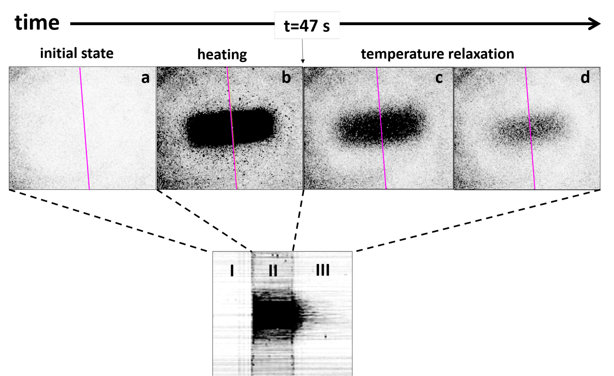
Images are taken before, during and after the sample heating. Therefore the undisturbed state of the beads, loss of the correlation and its following recovery have been tracked during the experiment. We recall that to obtain the correlation map, the images are first divided in metapixels and the correlation function are computed for each metapixel between two different states of the sample, here between two successive images. Maps of correlation function are done on zones of pixels, corresponding to speckles spots. An order of magnitude of the noise on depending on the size of the metapixel can be estimated using a uniform map obtained by two successive images of the undeformed sample. The ratio of the standard deviation and the mean value of for different choices of metapixel size is shown in Table 2.
| 4 pxl | |
|---|---|
| 8 pxl | |
| 16 pxl | |
| 32 pxl |
A size of pixels is a good compromise between the noise level and the final resolution of the correlation map. A length of pixels on the camera corresponds to .
The correlation maps corresponding to each phases of the experiment are shown in the upper part of the Fig. 11. They are presented in grayscale where the brightness of a pixel stands for the value of the correlation function. Map (a) has been obtained before the thermal deformation has been induced. It reveals the absence of any dynamics in the system and the value of the correlation function is close to 1. For all the pictures taken during the heating (e.g. map (b)), the signal coming from the illuminated zone is totally randomized and within this area the value of the correlation function drops to 0. The true magnitude of the decorrelation due to beads thermal expansion is not so large, however it is hidden under the emission of the white light. The proper values of the correlation in the system can be retrieved from the maps once the illumination is off (Fig. 11(c)). Then, the heat is conducted into the bulk of the sample balancing the temperature gradient along the sample surface. The activity in the system slows down and the correlation is getting recovered as it can be seen on map (d). It continues further and at some point the situation comes back to state (a).

Since the rate of the correlation recovery depends on the thermal diffusivity of a medium, this parameter can be retrieved from the obtained data. For that we monitor the variation of the correlation function along a slice of the correlation map passing through the heated zone. In Fig. 11 such a slice is indicated with the magenta line. The temporal fluctuation of the correlation function along this slice is presented in the bottom part of the figure by stacking the lines of the full recording in a spatio-temporal diagram. Here the number of pixel rows correspond to the length of the slice and the number of columns corresponds to the number of images taken during the experiment. The three phases of the experiment (before heating, during and after) are clearly seen in the stack and indicated as zones I, II and III, correspondingly. We are interested in zone III, where the recovery of the correlation occurs. Several profiles of the slices in zone III are plotted with circles in Fig. 12(a). Different colors corresponds to different images and therefore to different times. The profiles have been fitted with the Gaussian function for which the amplitude of the peak (noted as ) is associated with the magnitude of the thermal deformation and consequently with the temperature gradient. The amplitude decreases exponentially with time as shown in Fig. 12(b). The relaxation time can be measured: . It corresponds to the time of heat diffusion into the bulk. From reported values of thermal conductivity for glass beads [49] we may deduce a thermal diffusivity . We then find mm, which is in agreement with the probed depth into the sample which is few .
Such experiment can be easily implemented with standard lab equipment and allows to practice DWS measurement on a predictable configuration. In the next section, we present some examples of measurements that have been done on granular materials submitted to different kind of loading.
V Examples of applications
Here, we present briefly measurements that have been done in different configuration on granular samples. All the results presented in this section have been extensively described and discussed in other publications. We present them to illustrate the potential of the method.
V.1 Shear bands
A standard configuration to test failure of a granular material in soil mechanics is the biaxial test [50]: a sample submitted to a confining pressure is uniaxially compressed. It is also confined between two walls ensuring plane strain conditions (see Fig. 13(a)).

When the material fails it presents shear bands. Fig. 14(a) shows a typical correlation map obtained using DWS after the failure of the material displaying two conjugated shear bands. The mechanical response of the material can be schematically considered as solid blocks moving relatively as shown in the right part of Fig. 13.

We have performed in this experiment two complementary measurements: DWS measurements as described in the present review but also direct tracking of particles. The second method allows a direct measurement of the displacement field. An example of the average field is shown in Fig. 14(b). We observe that the displacement field obtained by tracking coincides with the strain map.
The results allow to show that the DWS method gives a measurement of relative displacements, explaining the fact that the part of the material that are in solid translation stay correlated in average. Indeed, a solid translation of 1 m of the scatterers results in a translation of the speckle pattern in the image plane of less than 3 % of a pixel. Consequently, the contribution of this translation to the decorrelation is negligible in this particular study. Nevertheless, it is possible to identify the solid translation of the speckle pattern complementary to its deformation in order to perform Particle Image Velocimetry [51].
V.2 Inclined plane: micro-ruptures
Another standard configuration for studying failure in a granular material is a progressive inclination a box filled with beads (see Fig. 15). The goal is then to identify the plastic mechanisms that precede the destabilization of the pile in an avalanche. In this system, small rearrangements as well as regular large micro-ruptures have been evidenced before the avalanche [55, 56, 57].

Our observations using DWS evidenced that localized rearrangements are present from the very beginning of the tilting process and occur at all depths in the sample. At a given depth, the density of the rearrangements increases with the shear, while at a given angle the density of the rearrangements decreases with the depth. We have also observed large events implying typically a part of the material parallel to the surface. Such micro-rupture can be seen in Fig. 16 at 25.63∘. The successive correlation maps surrounding the micro-rupture are shown. Those maps are incremental: they are computed between two successive speckle images. It is then possible to identify the details of the plastic processes at play during such micro-ruptures.

The micro-rupture phenomenology is mainly a function of the depth under the free surface so that a spatio-temporal representation obtained by averaging the values of the correlation at each depth allows a good visualization of the behavior of the sample during the quasi-static tilting of the pile (see Fig. 16(b)). We observe regularly spaced large events. The depth of those events increases linearly with the angle of inclination until the avalanche. Those events start from an angle typically around 15∘, independently from the type of material, revealing an internal threshold well below the avalanche angle.
An extensive study in this configuration can be found in Reference [57]. The unmatched resolution on deformation allows here to identify processes of very small amplitude. When studying precursors to catastrophic events, having access to such minute local deformation is crucial to resolve the internal plasticity before the failure.
V.3 Heterogeneous deformation: response to a localized force
An unsolved question in granular matter is the problem of the elastic limit of a non-cohesive granular material and of the response of this material when submitted to cycles of force of a very small amplitude. To separate the elastic, reversible, part from the plastic, irreversible one in DWS measurements, an image of reference can be used to compute all the correlations instead of studying only the incremental deformation between consecutive images. It is then possible to measure the recovered correlation during a cycle and to separate it from the irreversible loss of correlation during a cycle. To underline this difference in the present study in comparison to the previous ones we use a different colormap here: red corresponds to the maximal correlation () while dark blue corresponds to full decorrelation () (see colorscale in Fig. 18). In such study, a limitation can arise from the temporal stability of the laser that can limit the maximal time lag possible between two images. Typically, for non-stabilized HeNe or Nd:YAG lasers [18], the intensity correlation function decreased of 10% on a timescale of 100-1000 s. For studying very slow dynamics, the use of stabilized laser allows to keep a reference image for several hours. [36].
We have studied the mechanical response of a granular pile to a localized force and we have characterized experimentally the main differences between the response of the granular sample and the one of an elastic reference media [58]. The experimental setup is shown in Fig. 17.

The upper row of Fig. 18 shows the observed spatial repartition of the deformation in the sample during a force cycle for which we have observed a failure in the material. The reference image is the initial speckle image corresponding to the unloaded sample. We observe inhomogeneities in the otherwise regular response that we interpret as precursors of the rupture. As in the previous example, all the interest of DWS measurements is the possibility to study the intermittent heterogeneous dynamics that precedes the failure.

VI Conclusion
We have presented pedagogically how to measure deformation in granular materials using DWS. We have given the basic tools both on the theoretical side and on the very practical side for the reader to be able to implement this method in the lab. We have given a short review of the principle of Diffusing Wave Spectroscopy. We have discussed in more details the case of deformation in granular materials with special interest on how scattering take place in granular matter and how to take into account uncorrelated motion in addition to an affine deformation field when analysing the correlation functions. We have presented in details a tutorial experiments with practical tips on the adjustment of the setup. Finally we have briefly presented some observations done using this method in various experimental setups implying granular materials. This article should allows any beginner in the field to implement the method rapidly.
Acknowledgements
Part of the works presented here have been obtained during the PhD Theses of Marion Erpelding and Antoine Le Bouil as well as during the Master internship of Roman Bertoni. A. M. acknowledges postdoctoral financial support from ESA.
References
- [1] D. A. Weitz and D. J. Pine, in Dynamic Light Scattering : The Method and Some Applications. (Oxford University Press, 1993).
- [2] G. Maret, Curr. Opin. Colloid Interface Sci. 2, 251 (1997).
- [3] G Maret and P. E. Wolf, Z. Phys. B: Condens. Matter 65, 409 (1987).
- [4] D. J. Pine, D. A. Weitz, P. M. Chaikin, and E. Herbolzheimer, Phys. Rev. Lett. 60, 1134 (1988).
- [5] D. J. Durian, D. A. Weitz, and D. J. Pine, Science 252, 686 (1991).
- [6] R. Höhler, S. Cohen-Addad, and H. Hoballah, Phys. Rev. Lett. 79, 1154 (1997).
- [7] P. Hébraud, F. Lequeux, J. P. Munch, and D. J. Pine, Phys. Rev. Lett. 78, 4657 (1997).
- [8] N. Menon and D. J. Durian, Science 275, 1920 (1997).
- [9] R. Höhler, S. Cohen-Addad, and D. J. Durian, Curr. Opin. Colloid Interface Sci. 19, 242 (2014).
- [10] P. Zakharov and F. Scheffold, in Advances in dynamic light scattering techniques, (Springer Berlin Heidelberg, Berlin, Heidelberg, 2009).
- [11] L. Cipelletti, H Bissig, V Trappe, P Ballesta, and S Mazoyer, J. Phys.: Condens. Matter 15, S257 (2003).
- [12] P. Mayer, H. Bissig, L. Berthier, L. Cipelletti, J. P. Garrahan, P. Sollich, and V. Trappe, Phys. Rev. Lett. 93, 115701 (2004).
- [13] A. Duri, D. A. Sessoms, V. Trappe, and L. Cipelletti, Phys. Rev. Lett. 102, 085702 (2009).
- [14] P. K. Dixon and D. J. Durian, Phys. Rev. Lett. 90, 184302 (2003).
- [15] R. Bandyopadhyay, A. S. Gittings, S. S. Suh, P. K. Dixon, and D. J. Durian, Rev. Sci. Instrum. 76, 093110 (2005).
- [16] M. Erpelding, A. Amon, and J. Crassous, Phys. Rev. E 78, 046104 (2008).
- [17] P. Zakharov and F. Scheffold, Soft Materials 8, 102 (2010).
- [18] J. Crassous, J.-F. Metayer, P. Richard and C. Laroche, Journal of Statistical Mechanics: Theory and Experiment, 03, P03009 (2008).
- [19] D. A. Sessoms, H. Bissig, A. Duri, L. Cipelletti, and V. Trappe, Soft Matter 6, 3030 (2010).
- [20] J. C. Dainty ed., Laser Speckle and Related Phenomena (Springer-Verlag, Berlin, 1984).
- [21] P. K. Rastogi ed., Photomechanics (Springer-Verlag, Berlin, 2000).
- [22] M. Erpelding, B. Dollet, A. Faisant, J. Crassous, and A. Amon, Strain 49, 167 (2013).
- [23] D. J. Pine, in Light scattering and rheology of complex fluids driven far from equilibrium (SUSSP Institute of Physics, Bristol, 2000).
- [24] F. Scheffold and R. Cerbino, Curr. Opin. Colloid Interface Sci. 12, 50 (2007).
- [25] V. Viasnoff, F. Lequeux, and D. J. Pine, Rev. Sci. Instrum. 73, 2336 (2002).
- [26] M. Erpelding, PhD thesis, Thèse de doctorat, Université de Rennes 1, 2010.
- [27] A. Ishimaru, Wave Propagation and Scattering in Random Media (Academic Press, New York, 1978).
- [28] B. J. Berne and R. Pecora, Dynamic Light Scattering With Applications to Chemistery, Biology, and Physics (Dover Publication Inc., New York, 2000).
- [29] D. J. Pine, D. A. Weitz, J. X. Zhu, and E. Herbolzheimer, J. Phys. France, 51, 2101 (1990).
- [30] H. C. van de Hulst, Light scattering by small particles (Dover Publications, New York, 1981).
- [31] P. E. Wolf, G. Maret, E. Akkermans, and R. Maynard, J. Phys. France 49, 63 (1988).
- [32] Z. Sadjadi, M. Miri, M. R. Shaebani, and S. Nakhaee, Phys. Rev. E 78, 031121 (2008).
- [33] J. Crassous, Eur. Phys. J. E 23, 145 (2007).
- [34] P.-A. Lemieux and D. J. Durian, Phys. Rev. Lett. 85, 4273 (2000).
- [35] L. Djaoui and J. Crassous, Granul. Matter 7, 185 (2005).
- [36] J. Crassous, M. Erpelding, and A. Amon, Phys. Rev. Lett. 103, 013903 (2009).
- [37] W. Leutz and J. Rička, Opt. Commun. 126, 260 (1996).
- [38] D. Bicout, E. Akkermans, and R. Maynard, J. Phys. I 1, 471 (1991).
- [39] D. Bicout and R. Maynard, Physica A 199, 387 (1993).
- [40] D Bicout and G Maret, Physica A 210, 87 (1994).
- [41] X. L. Wu, D. J. Pine, P. M. Chaikin, J. S. Huang, and D. A. Weitz, J. Opt. Soc. Am. B 7, 15 (1990).
- [42] F. C. MacKintosh, J. X. Zhu, D. J. Pine, and D. A. Weitz, Phys. Rev. B 40, 9342 (1989).
- [43] A. Amon, V. B. Nguyen, A. Bruand, J. Crassous, and E. Clément, Phys. Rev. Lett. 108, 135502 (2012).
- [44] G. Petekidis, A. Moussaïd, and P. N. Pusey, Phys. Rev. E 66, 051402 (2002).
- [45] C. Baravian, F. Caton, J. Dillet, and J. Mougel, Phys. Rev. E 71, 066603 (2005).
- [46] J. D. Briers, Physiol. Meas. 22, R35 (2001).
- [47] L. Cipelletti and D. A. Weitz, Rev. Sci. Instrum. 70, 3214 (1999).
- [48] J. W. Goodman, Speckle phenomena in optics: theory and applications (Roberts and Company Publishers, Englewood, 2007).
- [49] J.-C. Géminard and H. Gayvallet, Phys. Rev. E 64, 041301 (2001).
- [50] J. Desrues and G. Viggiani, Int. J. Numer. Anal. Methods Geomech. 28, 279 (2004).
- [51] L. Cipelletti, G. Brambilla, S. Maccarrone, and S. Caroff, Opt. Express 19, 22353 (2013).
- [52] A. Le Bouil, A. Amon, J.-C. Sangleboeuf, H. Orain, P. Bésuelle, G. Viggiani, P. Chasle, and J. Crassous, Granul. Matter 16, 1 (2014).
- [53] A. Le Bouil, A. Amon, S. McNamara, and J. Crassous, Phys. Rev. Lett. 112, 246001 (2014).
- [54] T. B. Nguyen and A. Amon, EPL 116, 28007 (2016).
- [55] N. Nerone, M. A. Aguirre, A. Calvo, D. Bideau, and I. Ippolito, Phys. Rev. E 67, 011302 (2003).
- [56] S. Kiesgen de Richter, PhD thesis, Thèse de doctorat, Université de Rennes 1, 2009.
- [57] A. Amon, R. Bertoni, and J. Crassous, Phys. Rev. E 87, 012204 (2013).
- [58] M. Erpelding, A. Amon, and J. Crassous, EPL 91, 18002 (2010).