Importance Sampling of Rare Events in Chaotic Systems

For a chaotic system, $\lambda_{L}\equiv\lambda_{t\rightarrow\infty}>0$ in Eq. 6. The variation of the (maximum) finite-time Lyapunov exponents $\lambda_{t}$ (FTLE) across different initial conditions characterizes the variation of chaoticity of the system, yielding a distribution of the FTLE, $P(\lambda_{t_{o}})$, or, equivalently, the distribution of $E\equiv t_{o}\lambda_{t_{o}}$:

where $U(\boldsymbol{x})$ is a chosen probability distribution (e.g. uniform in the phase-space). The FTLE and its distribution was introduced in the 80s [25, 26, 27] and has been used to study turbulent flows [28], Hamiltonian dynamics [29], chimera states [30], characterize dynamical trapping [25, 31, 32, 33, 34], among others [35, 36]. The distribution of FTLE is related to the generalized dimensions [37] and often follows a large deviation principle, where $t_{o}$ is the extensive parameter [37, 18]. In strongly chaotic systems, the distribution of FTLE is Gaussian [37], whereas for intermittent chaos and other weakly chaotic systems the distribution is typically non-Gaussian [38].

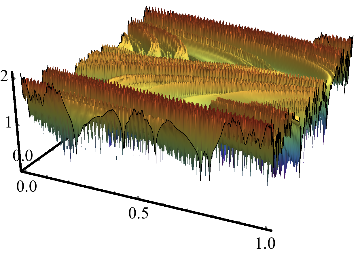
Figure 1 shows the phase-space dependency and distribution of the FTLE in one chaotic system. It contains characteristic features observed in strongly chaotic systems: $\lambda_{t}$ is a quantity that depends sensitively on the state $\boldsymbol{x}$, and its distribution $P(\lambda_{t})$ decays exponentially to zero on both sides. In the limit $t_{o}\rightarrow\infty$, $P(\lambda_{t_{o}})\rightarrow\delta(\lambda_{t_{o}}-\lambda_{L})$.

The tails of the distribution $P(E)$ play a significant role in the characterization of chaotic systems, as, for example, the higher moments of the distribution are related to higher $q$s in the generalized dimensions $D_{q}$ of the attractor [37]. Furthermore, the regions of the phase-space with small (large) finite-time Lyapunov exponent are associated with slow (fast) decay of correlations [27], and their characterization has been used to get insight on whether the system is ergodic or not [29]. Moreover, trajectories characterized by a low or high finite-time Lyapunov exponent can play a significant role in the dynamics of interfaces in chaotic flows [28] and others [16].

A typical analysis of the FTLE is to measure how a quantity, $W(\boldsymbol{x})$, depends on the FTLE $\lambda_{t_{o}}$ [27, 29, 28]. This requires estimating an integral of the form

where $W(\boldsymbol{x})$ is the pre-selected quantity, $\Gamma$ is a pre-selected sampling region (often $\Gamma=\Omega$), and $U(\boldsymbol{x})$ is the weight attributed to $\boldsymbol{x}$ (often uniform, $U(\boldsymbol{x})=1/|\Gamma|$). Let us look for two examples. First, consider the problem of estimating the distribution $P(\lambda_{t_{o}})$, e.g. Refs. [27, 29, 38, 16]. The traditional technique is to sample $M$ states $\boldsymbol{x}$ according to $U(\boldsymbol{x})=1/|\Gamma|$ and estimate $P(\lambda_{t_{o}})$ using the estimator $M_{\lambda}/M$, where $M_{\lambda}$ is the number of samples with $\lambda_{t_{o}}(\boldsymbol{x})\in[\lambda_{t_{o}},\lambda_{t_{o}}+\Delta\lambda_{t_{o}}]$. Formally, this corresponds to $W(\lambda_{t_{o}})$ with $W(\boldsymbol{x})=1$. The second example is retrieved from Ref. [27]. There, in order to evaluate the contribution of the algebraic region of the phase-space to the power spectra, the authors decomposed it in two terms corresponding to the power spectra of trajectories with low FTLE and trajectories with high FTLE. This required estimating the power spectra from a set of trajectories conditioned to an interval of $\lambda$s on the tails of the distribution. Associating the power spectrum ($S(f)$ in the ref.) with $W(\boldsymbol{x})=W_{f}(\boldsymbol{x})$ where $f$ is the frequency, the power spectra represented in Fig. 4 of Ref. [27] corresponds to integrals (for different frequencies $f$) given by

which contains integrals of the form of Eq. 10.

Numerically estimating the integral in Eq. 10 is challenging for two reasons: first, $P(\lambda_{t_{o}})$ decays with $t_{o}$ (lower panel of Fig. 1): the distribution of FTLE often follows a large deviation principle, $P(\lambda_{t_{o}}(\boldsymbol{x}))\propto\exp\left(t_{o}s(\lambda_{t_{o}})\right)$, where $s$ is intensive in respect to $t_{o}$ and is often concave [37]. Consequently, the traditional methodology of sampling states uniformly to find or sample states with increasing $t_{o}$ requires an exponentially high number of initial conditions. Second, the dependency of $\lambda_{t_{o}}(\boldsymbol{x})$ on $\boldsymbol{x}$ has multiple local minima and maxima (upper panel of Fig. 1). Such rough (fractal [39]) landscapes are known to challenge numerical techniques (e.g., simulations get trapped in local minima or maxima) [40].

The problem of finding and sampling states with high or low-$\lambda$ has been addressed in the literature with numerical techniques that go beyond traditional uniform sampling [16, 17, 18]. Such techniques have been successfully applied to find [16] and sample [17, 18] states with extremal $\lambda$s in different chaotic systems. Refs. [16, 18] use a population Monte Carlo canonical ensemble where $\lambda_{t}$ plays the role of the energy $E$ to find or sample states with high or low FTLE. The method computes stochastic trajectories that, from the numerical tests performed, are indistinguishable from (deterministic) trajectories of the system. Ref. [17] proposes a flat-histogram simulation to find high or low chaotic states by developing an observable to quantify the chaoticity of the state.

The best known examples of chaotic systems have a fractal attractor in the phase space [5], the Lorenz attractor being the most prominent example [6]. However, chaotic dynamics can appear also when the fractal invariant set in the phase space is not purely attracting, e.g. it may have stable and unstable directions (a saddle). Trajectories close to this set perform chaotic motion for an arbitrarily long (yet finite) time. This phenomenon appears in a variety of physical systems and is known as transient chaos [41, 42].

Numerical investigations of transiently-chaotic systems are computationally difficult because most trajectories quickly escape the vicinity of the chaotic saddle (on which the chaotic dynamics is properly defined) [12, 13, 43]. More precisely, the escape time of a state $\boldsymbol{x}$ in a pre-selected region $\boldsymbol{x}\in\Gamma\subset\Omega$ is defined as the first passage time of its trajectory to a pre-selected exit set $\Lambda\subset\Omega$:

Almost all trajectories start at $\Gamma$ and eventually leave when $\boldsymbol{x}_{t}\in\Lambda$, but they do so at different times $t_{e}$. Such variability is quantified by the distribution of escape time: the probability that a random initial condition $\boldsymbol{x}$ leaves at a given time $t_{e}$,

where $\delta_{t_{e},t_{e}(\boldsymbol{x})}$ is the Kronecker delta and $U(\boldsymbol{x})$ is the probability density assigned to each state in $\Gamma$, which is often constant, $U(\boldsymbol{x})=1/\int_{\Gamma}{\bf d}\boldsymbol{x}\equiv 1/|\Gamma|$. Figure 2 shows the typical features of $t_{e}(\boldsymbol{x})$: it strongly depends on the initial state $\boldsymbol{x}$ and its distribution $P(t_{e})$ decays exponentially to zero (i.e., it has a constant escape rate $\kappa$).

There are two main numerical techniques to study transiently chaotic systems. The first is to find one long living state $\boldsymbol{x}$ with $t_{e}(\boldsymbol{x})\gg 1$ and to compute an average over states of this trajectory [11, 12]. For large $t_{e}(\boldsymbol{x})$, the trajectory between times $[t_{e}(\boldsymbol{x})/2-t_{s},t_{e}(\boldsymbol{x})/2+t_{s}]$ where $t_{s}\ll t_{e}(\boldsymbol{x})/2$ is close to a trajectory on the chaotic saddle. When the saddle is ergodic, an average over this long trajectory corresponds to an average over the natural invariant density and therefore an average over these states characterizes invariant properties of the system. The second technique, which we focus in this work, is to compute averages over an ensemble $U(\boldsymbol{x})$ of initial conditions $\boldsymbol{x}$ that leave the system at time $t_{e}(\boldsymbol{x})=t_{e}$ [11, 42]. For small $t_{e}$ observations depend on the particular initial density $U(\boldsymbol{x})$ (a point of interest in itself [42]), while for large $t$ they characterize invariant properties of the system (like in the previous technique, the states $\boldsymbol{F}^{t/2}(\boldsymbol{x})$ with $t\rightarrow\infty$ are independent samples of the natural invariant density).

A typical analysis within sampling transiently chaotic systems is to measure how a quantity, $W(\boldsymbol{x})$, changes with increasing escape time $t_{e}$. Numerically, this can be written as

Let us enumerate 3 examples of computational problems that can be interpreted as numerical estimations of an integral of the form of $W(t_{e})$ in Eq. 14.

To provide an unified treatment of the numerical problems in transient chaos and in computing FTLE of closed systems we use a common notation whenever possible. It indicates also how the methods can be generalized to different problems. Firstly, there is a quantity that we call ”observable” and denote by $E(\boldsymbol{x})$:

• •

  $E(\boldsymbol{x})=t_{o}\lambda_{t_{o}}(\boldsymbol{x})$ in FTLE of closed systems

• •

  $E(\boldsymbol{x})=t_{e}(\boldsymbol{x})$ in strongly chaotic open systems

Secondly, we use $\delta(E,E^{\prime})$ to denote both the Kronecker delta and the Dirac delta ($\delta(E-E^{\prime})$), for discrete and continuous case respectively. This is needed because, even though in practice we will always consider $E$ to be a discrete function due to binning of the histograms, formally the observable $E$ is either discrete ($t_{e}$ for maps) or continuous ($\lambda_{t}$ or $t_{e}$ for flows). Thirdly, the observable $E$ is a function of the phase-space of the system but typically depends also on an external quantity $N$ that parameterizes how high $E$ can be:

• •

  $t_{o}$ in FTLE of closed systems

• •

  (a pre-selected) maximum escape time, $t_{\max}$, in strongly chaotic open systems.

This parameter is important to us because, the higher it is, the rarer a state with the maximum or minimum possible $E$ is. In this notation, the two general problems presented in the previous sections can be summarized as follows:

• •

  the analysis is conditioned to a projection of $\boldsymbol{x}$ into a one-dimensional observable $E(\boldsymbol{x})$.

• •

  the probability distribution of $E$, $P(E)$, decays exponentially with increasing $E$.

• •

  the focus of the analysis is on rare states in respect to $P(E)$: states with $E$ in one of the tails of $P(E)$.

• •

  the rareness increases with $N$.

In transient chaos problems we are interested in states with increasing $N=t_{\max}$ that correspond to the tail of $P(E)=P(t_{e})$, $P(t_{\max})$. In computations of the FTLE in closed systems we are interested in states with increasing $N=t_{o}$ and on the tails of $P(E)$. These problems share two distinct computational problems: find rare states [12, 13, 11, 16] and sample rare states [17, 18, 45, 46], which can be formalized as follows:

• •

  Find rare states: minimize or maximize $E(\boldsymbol{x})$ over a constraining region $\Gamma$, $\boldsymbol{x}\in\Gamma\subset\Omega$, for increasing $N$.

• •

  Sample rare states: compute the integral of a function $W(\boldsymbol{x})$ conditioned to a particular value of $E$ and for increasing $N$, over an ensemble of states $\boldsymbol{x}$ distributed according to $U(\boldsymbol{x})$ in a constraining region of the phase-space $\boldsymbol{x}\in\Gamma\subset\Omega$:

  $$W(E)=\int_{\Gamma}W(\boldsymbol{x})\delta(E,E(\boldsymbol{x}))U(\boldsymbol{x}){\bf d}\boldsymbol{x}\ \ .$$

  (16)

The numerical challenges of these two numerical problems are common: the states $\boldsymbol{x}$ are exponentially difficult to find with increasing $N$ (or $E$), the function $E(\boldsymbol{x})$ contains multiple local and global minima embedded in fractal-like structures, and a potential high dimensionality $D$ of the phase-space (see Figs. 1 and 2). The goal of this paper is to develop a systematic approach to tackle the two numerical problems and these three challenges.

As described in the previous section, the traditional methodology to compute an integral of the form of Eq. 16 is to draw $m$ samples $\{\boldsymbol{x}_{i}\}$ distributed according to $U(\boldsymbol{x})$ from the relevant region $\Gamma$ and approximate the integral $W(E)$ by the estimator

where $\delta(E,E(\boldsymbol{x}))=1$ when $E(\boldsymbol{x}_{i})\in[E,E+\Delta E[$ and zero otherwise (when E is discrete, $\Delta E=1$). The relative distance of the estimator $\overline{W(E)}$ to $\mathbb{E}\left[W(E)\right]$ is quantified by the ratio $\epsilon(E)\equiv\sigma\left[\overline{W(E)}\right]/\mathbb{E}\left[W(E)\right]$ where $\sigma\left[\overline{W(E)}\right]^{2}\equiv\mathbb{E}\left[\overline{W(E)}^{2}\right]-\mathbb{E}\left[\overline{W(E)}\right]^{2}$. For the estimator in Eq. 17, this is given by

where $G(E)$ is the density of states: the number of states per bin with an observable $E$.²² 2 $G(E)=P(E)$ when each state is equally weighted, $U(\boldsymbol{x})=1/|\Gamma|$. Therefore, the number of samples $m_{*}$ required to achieve a given precision $\epsilon_{*}$ for a given $E_{*}$ is $m_{*}(E_{*})\propto 1/G(E_{*})$. The critical problem in sampling rare states is that, because $G(E)$ decays exponentially with $E$, $m_{*}(E)$ increases exponentially with $E$.

Importance sampling techniques aim to improve this scaling by drawing samples from a distribution $\pi(\boldsymbol{x})\neq U(\boldsymbol{x})$ on the phase-space (e.g. non-uniformly in the phase-space) [8]. Specifically, consider $m$ independent samples $\{\boldsymbol{x}_{i}\}$ drawn from $\pi(\boldsymbol{x})$, and the function $\pi(\boldsymbol{x})$ to depend only on $E$, $\pi(\boldsymbol{x})=\pi(E(\boldsymbol{x}))=\pi(E)$. Because the samples are not drawn from $U(\boldsymbol{x})$, the estimator in Eq. 17 would be biased. Importance sampling uses an unbiased estimator for $W(E)$ given by [8]

which reduces to Eq. 17 when $\pi(\boldsymbol{x})=U(\boldsymbol{x})$. The advantage of importance sampling is that the relative error of the estimator in Eq. 19 is given by

This is because, when sampling from $\pi(\boldsymbol{x})=\pi(E(\boldsymbol{x}))$, the expected number of samples with a given $E$, $m(E)$, is equal to

Equation 20 implies that the function $\pi(E)$ can be chosen to favour states $\boldsymbol{x}$ with observable $E$ on the tails of $G(E)$ and therefore improve the precision of the estimator on these tails.

The standard deviations in Eqs. 18,20 were obtained assuming that the $m$ samples were independent. In traditional methodologies such as uniform sampling, this is the case. However, in the algorithms discussed below, it is not. Therefore, it is necessary to modify Eq. 20 for the case where the samples $\{\boldsymbol{x}_{i}\}$ are drawn from $\pi(\boldsymbol{x})$ and are also correlated. This modification is given by

where $T(E)$ is the autocorrelation time [8], which increases with the correlation of the samples.

Efficient importance-sampling [7, 8, 9] techniques have to address the following three steps:

1. 1.

   choose a suitable $\pi(\boldsymbol{x})$

2. 2.

   have a method to generate samples from $\pi(\boldsymbol{x})$

3. 3.

   minimize the autocorrelation time $T$

A defining point in our method is our choice for the Metropolis-Hasting algorithm to address point 2, differently from Refs. [16, 20] which address similar problems through a different choice for point 2 (cloning trajectories). Below we first discuss point 2, then point 1, and finally point 3.

The Metropolis-Hastings (MH) algorithm asymptotically generates states $\boldsymbol{x}$ according to $\pi(\boldsymbol{x})$ using a a Markovian, ergodic and detailed balance random walk in the sampling region $\Gamma$ [8]. This random walk is initialized from a random state $\boldsymbol{x}\in\Gamma$ and evolves to a new state $\boldsymbol{x}^{\prime}\in\Gamma$ with a transition probability $P(\boldsymbol{x}^{\prime}|\boldsymbol{x})$ chosen such that asymptotically the states $\boldsymbol{x}$ are drawn according to $\pi(\boldsymbol{x})$. In Metropolis-Hastings, $P(\boldsymbol{x}^{\prime}|\boldsymbol{x})$ is written as

where $g(\boldsymbol{x}^{\prime}|\boldsymbol{x})$ is the (proposal) distribution used to generate new states and $a(\boldsymbol{x}^{\prime}|\boldsymbol{x})$ is the (acceptance) distribution used to select them. The random walk fulfills detailed balance because the acceptance probability is chosen as [8]

Metropolis-Hastings algorithm is not the only way to achieve this. Another popular and alternative method to sample from $\pi(\boldsymbol{x})$ is population Monte Carlo, which instead of a random walk, uses multiple stochastic trajectories that are cloned and destroyed. See e.g. ref. [18] for an application to the problem of the FTLE described above.

Algorithmically, the MH algorithm is implemented as follows: choose a region $\Gamma$ and a random initial condition $\boldsymbol{x}\in\Gamma$. Evolve the random walk in time according to:

1. 1.

   Propose a state $\boldsymbol{x}^{\prime}$ drawn from $g(\boldsymbol{x}^{\prime}|\boldsymbol{x})$;

2. 2.

   Compute $a(\boldsymbol{x}^{\prime}|\boldsymbol{x})$ replacing $\boldsymbol{x}$ and $\boldsymbol{x}^{\prime}$ in Eq. 23;

3. 3.

   Generate a random number $r$ in $[0,1]$. If $r<a(\boldsymbol{x}^{\prime}|\boldsymbol{x})$, make $\boldsymbol{x}^{\prime}$ to be the new $\boldsymbol{x}$;

4. 4.

   Store $\boldsymbol{x}$ and go to 1.

The set of sub-steps 1-4 brings the random walk from its current state $\boldsymbol{x}$ to the next state and it is called a Markov step. After a transient number of steps where the algorithm converges to the asymptotic distribution, the stored states $\boldsymbol{x}$ are (correlated) samples drawn from $\pi(\boldsymbol{x})$, and can be directly used in Eq. 19.

The relative error $\epsilon(E)$ depends on the value of $N$ and on the particular value of $E/N$. To avoid discussing the dependency on $E/N$, the efficiency of the flat-histogram is often quantified in terms of the average round-trip [58, 59, 60], which is an upper bound for the number of Markov steps $m$ (samples) required to obtain an uncorrelated sample from $\pi(\boldsymbol{x})$ [61, 60]. The round-trip, $\tau$, is the average number of steps required for the algorithm to go from a state $\boldsymbol{x}$ with $E(\boldsymbol{x})=E_{\min}$ to a state $\boldsymbol{x}$ with $E(\boldsymbol{x})=E_{\max}$ and return back. ³³ 3 Numerically, the round-trip time is computed by having a boolean value tracking whether the random walk is moving in the direction $E_{\min}\rightarrow E_{\max}$ or $E_{\max}\rightarrow E_{\min}$, and use it to measure the total number of steps required to make the full round-trip. Ref. [45] shows how the autocorrelation time of a canonical ensemble is related to the autocorrelation time of a flat-histogram, and therefore we will use here the round-trip time of a flat-histogram simulation to quantify the efficiency for both distributions. The uniform sampling has a round-trip that increases exponentially with $N$: on average it takes $1/G(E_{\max})$ samples to get one sample with $E_{\max}$, and $1/G(E_{\max})$ increases exponentially with $N$.

Importance sampling Monte Carlo is widely used in statistical physics because the computational cost often scales polynomially with $N$ [60, 8], which is a dramatic improvement over uniform sampling. Under the hypothesis that (a) $\Delta E\equiv E(\boldsymbol{x}^{\prime})-E(\boldsymbol{x})\approx 1\ll N$ and (b) the correlation between the different $E(\boldsymbol{x})$ of the random walk decay fast enough, it can be shown that the roundtrip $\tau$ scales as [60, 46]

For example, consider the problem of sampling states of an open chaotic system with different escape times $t_{e}$ from $t_{e}=1$ up to $t_{e}=t_{e}^{\max}$. In this case, $E_{\min}=1$ and $E_{\max}=N=t_{e}^{\max}$. Thus, under the hypothesis (a) and (b) above, the round-trip is expected to scale as

There are known deviations of the scaling in Eq. 28 leading to a higher exponent, $N^{2+z}$ with $z>0$ [58, 59, 60, 46] and there are two common situations where this happens: (1) the acceptance rate decreases drastically with $N$ (hypothesis (a) above is violated); (2) autocorrelation drastically increases with $N$ (hypothesis (b) above is violated) [60, 46]. Nevertheless, these do not qualitatively change the argument: Monte Carlo with flat-histogram has the potential of generating rare states polynomially with increasing $N$, while uniform sampling generates rare states exponentially with increasing $N$.

To achieve a MH algorithm that scales polynomially with N, the autocorrelation time needs to be low. A key ingredient for an efficient algorithm is a good proposal distribution $g(\boldsymbol{x}^{\prime}|\boldsymbol{x})$ [63]. The ideal proposal distribution of a Metropolis-Hastings algorithm draws $\boldsymbol{x}^{\prime}$ independently of $\boldsymbol{x}$ according to $\pi(\boldsymbol{x}^{\prime})$, $g(\boldsymbol{x}^{\prime}|\boldsymbol{x})=\pi(\boldsymbol{x}^{\prime})$. This is because i) the acceptance in Eq. 23 is always one and ii) each step of the random walk generates an independent sample $\boldsymbol{x}$, which implies that the error in Eq. 22 is minimal. The difficulty of sampling rare events in chaotic systems is that a useful $\pi(\boldsymbol{x})$ to sample them is a difficult function to sample from. For concreteness, consider the problem of sampling high escape times in the open tent map defined in Appendix VII.1.3 – Eq. 66, whose $t_{e}(\boldsymbol{x})$ is represented in Fig. 12 – and consider the canonical sampling distribution, $\pi(\boldsymbol{x})\propto\exp(-\beta t_{e}(\boldsymbol{x}))$. In this example, $\pi(\boldsymbol{x})\propto\exp(-\beta 1)$ between $[1/a,1-1/a]$ and so forth ($\exp(-\beta t_{e})$) in subsequent intervals. The number of intervals increases as $2^{t_{e}}$. Therefore, sampling from $\pi(\boldsymbol{x})$ would require enumerating every interval, sample one at random according to a correct distribution that depends on $\beta$, and then sample a uniform point within that interval. While this can be done in simple maps such as the open tent map, this is unfeasible in a general system where the $t_{e}(\boldsymbol{x})$ dependency is unknown.

One way to approach the problem could be to consider $g(\boldsymbol{x}^{\prime}|\boldsymbol{x})$ to be the uniform distribution over $\Gamma$. One could imagine that changing the sampling distribution $\pi(\boldsymbol{x})$ could decrease the variance of the estimator, since this gives more preference to rarer states. However, this is not the case: changing the sampling distribution alone does not decrease the scaling of the variance of the estimator. This is because changing the sampling distribution (e.g. using a canonical ensemble) leads to an exponential increase of the autocorrelation time $T(E)$ with $E$, see Appendix VII.2, making it as efficient as traditional uniform sampling.

In summary, Metropolis-Hastings is an excellent candidate to approach the numerical challenges found in the study of rare events in chaotic systems. Firstly, because it is grounded in strong mathematical results such as importance sampling theorem and asymptotic convergence of Markov processes. Secondly, because it is formulated with very little assumptions about the system, the observable of interest or the dynamics of the system, which gives enough freedom to adapt it to the specific aim (sampling or finding), observable, and system. Thirdly, because there seems to be no theoretical reason for the sampling to be exponential; Metropolis-Hastings is used to sample rare states in polynomial time in other problems of statistical physics. Finally, because the numerical problems found in chaotic systems can be re-written as problems where Metropolis-Hastings is suitable for. On the other hand, the optimal proposal of Metropolis-Hastings is unfeasible in chaotic systems, and without any extra information about the system, Metropolis-Hastings is as efficient as the traditional uniform sampling.

The goal of the proposal distribution $g(\boldsymbol{x}^{\prime}|\boldsymbol{x})$ we construct here will be to bound the acceptance rate in Eq. 23 away from 0 and 1. Since $a(\boldsymbol{x}^{\prime}|\boldsymbol{x})$ in Eq. 23 depends on $\boldsymbol{x}^{\prime}$, it is essential to look at its expectation over the proposal,

Our goal is to construct a proposal distribution such that⁴⁴ 4 E.g. Ref. [63] computed $a_{\star}=0.234$.

The motivation to set this as the starting point (and cornerstone) of our method is that it avoids the two typical origins of high correlation times $T$. When the acceptance is low, $T$ increases because the method remains stuck in the same state $\boldsymbol{x}$ for long times. High acceptance typically indicates that $\boldsymbol{x}^{\prime}$ is too close to $\boldsymbol{x}$ (often $E(\boldsymbol{x}^{\prime})=E(\boldsymbol{x})$), which implies that the simulation moves too slowly (in $E$ and in $\Omega)$. The goal here is not that the acceptance is exactly $a_{\star}$, but rather that it remains bounded from the extremes and that it does not strongly depend on $N$.

In general it is non-trivial to construct a proposal distribution that guarantees a constant acceptance. Thus, the next step is to approximate Eq. 31 by a simpler condition. Let us first notice that $\pi(\boldsymbol{x})$ only depends on $\boldsymbol{x}$ through $E_{\boldsymbol{x}}\equiv E(\boldsymbol{x})$, $\pi(\boldsymbol{x})=\pi(E_{\boldsymbol{x}})$. Therefore, at the very least, the proposal $g(\boldsymbol{x}^{\prime}|\boldsymbol{x})$ should guarantee that $\boldsymbol{x}^{\prime}$ is generated from $\boldsymbol{x}$ in such a way that $\pi(E_{\boldsymbol{x}^{\prime}})$ is neither too close (high acceptance) nor too far (low acceptance) from $\pi(E_{\boldsymbol{x}})$. Quantitatively, this can be written as

where $0<a<1$ is a constant. When the proposal is able to achieve a small variation of $E$, $\pi(E_{\boldsymbol{x}^{\prime}})$ can be expanded in Taylor series around $E_{\boldsymbol{x}^{\prime}}=E_{\boldsymbol{x}}$, which allows to write

Inserting Eq. 33 in Eq. 32, an average constant acceptance is thus achieved when

This equation, the main result of this section, is a condition that an efficient Metropolis-Hastings imposes to the proposal distribution in terms of the average difference in the observable $E$. This condition is non-trivial because it depends on the particular $\pi$, $E$, $\boldsymbol{F}$, and $\boldsymbol{x}$. For the sampling distributions discussed in the previous section, we obtain:

The proposal distribution requires correlating the trajectory starting at $\boldsymbol{x}^{\prime}$ with a trajectory starting at $\boldsymbol{x}$ such that Eq. 34 holds. Fulfilling this requirement requires the ability to control $\mathbb{E}\left[E_{\boldsymbol{x}^{\prime}}-E_{\boldsymbol{x}}|\boldsymbol{x}\right]$, which requires a procedure to correlate the state $\boldsymbol{x}^{\prime}$ with $\boldsymbol{x}$. The aim of this section is to introduce a quantification of the correlation of two trajectories of finite-time $t_{o}$ that can be related with $\mathbb{E}\left[E_{\boldsymbol{x}^{\prime}}-E_{\boldsymbol{x}}|\boldsymbol{x}\right]$, and present two different proposal distributions that propose a state $\boldsymbol{x}^{\prime}$ on which this correlation is controlled.

The observables $E$ introduced in section II.3 are all dependent not only of $\boldsymbol{x}$, but also of the full trajectory of length $t_{o}$ starting $\boldsymbol{x}$.⁶⁶ 6 The escape time $t_{e}$ requires that $\boldsymbol{F}^{t}(\boldsymbol{x})\notin\Lambda\ \ ,\forall t$; the FTLE $\lambda_{t_{o}}$ is a sum of terms computed over the trajectory. One natural way to quantify the similarity of two trajectories is the length the two trajectories remain within a distance $\Delta$ much smaller than a characteristic length of $\Gamma$. Formally, this can be quantified by $t_{\star}(\boldsymbol{x},\boldsymbol{x}^{\prime})=\max\{t\leq t_{o}:|\boldsymbol{F}^{t}(\boldsymbol{x})-\boldsymbol{F}^{t}(\boldsymbol{x}^{\prime})|\leq\Delta\}$. Under this definition, $0\leq t_{\star}(\boldsymbol{x},\boldsymbol{x}^{\prime})\leq t_{o}$. When $\boldsymbol{x}^{\prime}=\boldsymbol{x}$, $t_{\star}(\boldsymbol{x},\boldsymbol{x}^{\prime})=t_{o}$ because the trajectories are the same; when $\boldsymbol{x}^{\prime}$ is far from $\boldsymbol{x}$, $t_{\star}(\boldsymbol{x},\boldsymbol{x}^{\prime})=0$. However, there is another possibility for two trajectories starting at $\boldsymbol{x}^{\prime}$ and $\boldsymbol{x}$ to be similar: when the two trajectories are similar apart from a shift in time, see right panel of figure 3. One way to include both cases in our measure of similarity is to define $t_{\star}(\boldsymbol{x},\boldsymbol{x}^{\prime})$ as

For ${t_{\text{shift}}}=0$, this recovers the case of two trajectories starting close to each other; ${t_{\text{shift}}}\neq 0$, it includes situations where a trajectory starts at $\boldsymbol{x}^{\prime}$ close to $\boldsymbol{F}^{{t_{\text{shift}}}}(\boldsymbol{x})$.

This definition is motivated by the concept of symbolic sequences. [5] The similarity of the trajectory starting from $\boldsymbol{x}^{\prime}$ with the one starting from $\boldsymbol{x}$ can be quantified by the number of symbols that both trajectories share, which corresponds to the $t_{\star}(\boldsymbol{x},\boldsymbol{x}^{\prime})$ in Eq. 37. The definition in Eq. 37 avoids the necessity of the existence of a phase-space partition, but, for the purposes of the argument below, the two trajectories share a sequence of $t_{\star}$ states that are close within $\Delta$.

The average correlation between two states whose one is drawn according to a proposal distribution is here defined by

Notice that this quantity does not depend on the particular sampling distribution or algorithm; it is a function of the proposal distribution and the state $\boldsymbol{x}$. The goal of the next sub-sections is to construct proposal distributions that guarantee a given average correlation $t_{\star}(\boldsymbol{x})$. We will show, for example, that we can enforce an average correlation $t_{\star}(\boldsymbol{x})$ if we use a normal distribution centered around $\boldsymbol{x}$ with a specific standard deviation as our proposal distribution.

References

- [1] J. C. Leitão, “A library to sample chaotic systems,” https://github.com/jorgecarleitao/chaospp (2017).
- [2] S. Albeverio, V. Jentsch, and H. Kantz, Extreme Events in Nature and Society (Springer, 2006).
- [3] P. Holmes, Physics Reports 193, 137 (1990).
- [4] A. E. Motter and D. K. Campbell, Physics Today 66, 27 (2013).
- [5] E. Ott, Chaos in Dynamical Systems, 2nd ed. (Cambridge University Press, Cambridge, 1993).
- [6] E. N. Lorenz, Journal of the Atmospheric Sciences 20, 130 (1963).
- [7] M. E. J. Newman and G. T. Barkema, Monte Carlo Methods in Statistical Physics (Oxford University Press, USA, New York, 2002).
- [8] C. P. Robert and G. Casella, Monte Carlo statistical methods, 2nd ed., Springer texts in statistics (Springer, Berlin, 2005).
- [9] J. A. Bucklew, Introduction to rare event simulation, Springer series in statistics (Springer, New York, 2004).
- [10] V. Lucarini, D. Faranda, A. C. M. Freitas, J. M. Freitas, T. Kuna, M. Holland, M. Nicol, M. Todd, and S. Vaienti, arxiv (2016), arXiv:1605.07006 .
- [11] Y.-C. Lai and T. Tél, Transient chaos: Complex dynamics in finite time scales, 1st ed., edited by S. S. Antman, J. E. Marsden, and L. Sirovich, Vol. 173 (Springer, New York, 2010).
- [12] D. Sweet, H. E. Nusse, and J. A. Yorke, Physical Review Letters 86, 2261 (2001).
- [13] E. M. Bollt, International Journal of Bifurcation and Chaos 15, 1615 (2005).
- [14] C. Dellago, P. G. Bolhuis, and P. L. Geissler, Advances in Chemical Physics (2002).
- [15] P. G. Bolhuis, D. Chandler, C. Dellago, and P. L. Geissler, Annual review of physical chemistry 53, 291 (2002).
- [16] J. Tailleur and J. Kurchan, Nature Physics 3, 203 (2007).
- [17] A. Kitajima and Y. Iba, Computer Physics Communications 182, 251 (2011).
- [18] T. Laffargue, K.-D. N. T. Lam, J. Kurchan, and J. Tailleur, Journal of Physics A: Mathematical and Theoretical 46, 254002 (2013).
- [19] S. Patra and S. Keshavamurthy, Chemical Physics Letters 634, 1 (2015).
- [20] J. Wouters and F. Bouchet, J. PHys. A:Math. Theor. 49, 374002 (2016).
- [21] P. Geiger and C. Dellago, Chemical Physics 375, 309 (2010).
- [22] M. Grünwald, C. Dellago, and P. L. Geissler, The Journal of chemical physics 129, 194101 (2008).
- [23] P. Cvitanovic, R. Artuso, R. Mainieri, G. Tanner, and G. Vattay, Chaos book (Niels Bohr Institute, Copenhagen, 2016).
- [24] This is sometimes denoted as the stability exponent. See Chapter 4 and 6 of Ref. [23].
- [25] P. Grassberger and H. Kantz, Physics Letters A 113, 167 (1985).
- [26] P. Grassberger, R. Badii, and A. Politi, Journal of Statistical Physics 51, 135 (1988).
- [27] M. Sepúlveda, R. Badii, and E. Pollak, Physical review letters 63, 1226 (1989).
- [28] D. Beigie, A. Leonard, and S. Wiggins, Physical Review Letters 70, 275 (1993).
- [29] C. Amitrano and R. Berry, Physical review letters 68, 729 (1992).
- [30] S. Olmi, Chaos 25, 123125 (2015).
- [31] G. Zaslavsky, Physica D: Nonlinear Phenomena 168-169, 292 (2002).
- [32] J. Szezech, S. Lopes, and R. Viana, Physics Letters A 335, 394 (2005).
- [33] R. Artuso and C. Manchein, Physical Review E 80, 036210 (2009).
- [34] C. Manchein, M. W. Beims, and J. M. Rost, Chaos (Woodbury, N.Y.) 22, 033137 (2012).
- [35] H. D. I. Abarbanel, R. Brown, and M. B. Kennel, Journal of Nonlinear Science 1, 175 (1991).
- [36] H. D. I. Abarbanel, R. Brown, and M. B. Kennel, Journal of Nonlinear Science 2, 343 (1992).
- [37] C. Beck and F. Schögl, Thermodynamics of chaotic systems: an introduction (Cambridge University Press, 1995).
- [38] A. Prasad and R. Ramaswamy, Physical Review E 60, 2761 (1999).
- [39] H. Richter, “Scale-invariance of ruggedness measures in fractal fitness landscapes,” (2016), arXiv:1612.07029 .
- [40] U. H. E. Hansmann and Y. Okamoto, Journal of Computational Chemistry 14, 1333 (1993).
- [41] T. Tél and Y.-C. Lai, Physics Reports 460, 245 (2008).
- [42] E. G. Altmann, J. S. E. Portela, and T. Tél, Reviews of Modern Physics 85, 869 (2013).
- [43] M. Sala, J. C. Leitão, and E. G. Altmann, Chaos: An Interdisciplinary Journal of Nonlinear Science 26, 123124 (2016).
- [44] M. Dhamala, Y. C. Lai, and E. J. Kostelich, Physical review. E, Statistical, nonlinear, and soft matter physics 64, 056207 (2001).
- [45] J. C. Leitão, J. M. V. P. Lopes, and E. G. Altmann, Physical Review Letters 110, 220601 (2013).
- [46] J. C. Leitão, J. M. V. P. Lopes, and E. G. Altmann, Physical Review E 90, 052916 (2014).
- [47] when each state is equally weighted, .
- [48] G. Torrie and J. Valleau, Journal of Computational Physics 23, 187 (1977).
- [49] R. H. Swendsen and J.-S. Wang, Physical Review Letters 57, 2607 (1986).
- [50] E. Marinari and G. Parisi, Europhysics Letters (EPL) 19, 451 (1992).
- [51] Y. Sugita and Y. Okamoto, Chemical Physics Letters 314, 141 (1999).
- [52] J. Lee, Physical review letters 71, 211 (1993).
- [53] B. A. Berg and T. Neuhaus, Physics Letters B 267, 249 (1991).
- [54] F. Wang and D. P. Landau, Physical Review Letters 86, 2050 (2001).
- [55] J. Viana Lopes, M. Costa, J. Lopes dos Santos, and R. Toral, Physical Review E 74, 046702 (2006).
- [56] C. G. Zhou and R. N. Bhatt, Physical Review E 72, 025701 (2005).
- [57] R. E. Belardinelli, S. Manzi, and V. D. Pereyra, Physical Review E 78, 067701 (2008).
- [58] S. Trebst, D. A. Huse, and M. Troyer, Physical Review E 70, 046701 (2004).
- [59] P. Dayal, S. Trebst, S. Wessel, D. Wurtz, M. Troyer, S. Sabhapandit, and S. N. Coppersmith, Physical Review Letters 92, 097201 (2004).
- [60] J. Viana Lopes, Métodos de Monte Carlo para sistemas com desordem e interacção de longo alcance, Ph.D. thesis, Universidade do Porto (2006).
- [61] M. D. Costa, J. V. Lopes, and J. M. B. L. dos Santos, Europhysics Letters (EPL) 72, 802 (2005).
- [62] Numerically, the round-trip time is computed by having a boolean value tracking whether the random walk is moving in the direction or , and use it to measure the total number of steps required to make the full round-trip.
- [63] G. O. Roberts, A. Gelman, and W. R. Gilks, The Annals of Applied Probability 7, 110 (1997).
- [64] E.g. Ref. [63] computed .
- [65] In statistical physics an heuristics often used in Metropolis-Hastings is . E.g. it is used in the derivation of Eq. 28, and has been used for example in spin systems (single spin flip) [60], ensemble of complex networks (single link exchange) [Fischer2015], and proteins [Grassberger1997].
- [66] The escape time requires that ; the FTLE is a sum of terms computed over the trajectory.
- [67] An exponential distribution would be equally acceptable and would not change the main conclusions.
- [68] C. Grebogi, S. Hammel, J. Yorke, and T. Sauer, Physical Review Letters 65, 1527 (1990).
- [69] This equation is strictly valid for 1D, but the idea is that we split the FTLE between a component up to and the remaining component.
- [70] In Ref. [46] we used , different from Eq. 54. The derivation of Eq. 54 uses stronger approximations than the derivation of . See argumentation after Eq. (14) of Ref. [46].
- [71] Y. Iba, N. Saito, and A. Kitajima, Annals of the Institute of Statistical Mathematics 66, 611 (2014).
- [72] For example, using this heuristics, in a Metropolis-Hastings flat-histogram in the Ising model (in this case corresponds to a list of all spins, corresponds to the energy of the configuration), when the configuration of the system is close to the maximum of the density of states (maximal energy, no magnetization), there is no need to flip just one spin at the time: one can flip all spins at once because, there, correlating such states brings no advantage to increase the acceptance rate (it is going to be accepted anyway), but it increases .
- [73] M. Grünwald, Transition path sampling simulations of structural phase transformations in nanocrystals under pressure, Ph.D. thesis, University of Wien (2009).
- [74] C. N. Rowley and T. K. Woo, The Journal of Chemical Physics 131, 234102 (2009).
- [75] N. Eidelson and B. Peters, The Journal of Chemical Physics 137, 094106 (2012).
- [76] B. Schaefer, S. Mohr, M. Amsler, and S. Goedecker, The Journal of Chemical Physics 140, 214102 (2014).
- [77] J. C. Leitão, Ph.D. Thesis, TU Dresden (Germany) (2016).