On Optimal Spectrum Access of Cognitive Relay With Finite Packet Buffer Thanks: Copyright (c) 2015 IEEE. Personal use of this material is permitted. However, permission to use this material for any other purposes must be obtained from the IEEE by sending a request to pubs-permissions@ieee.org.

Kedar Kulkarni Adrish Banerjee ^†^†thanks: The authors are with Department of Electrical Engineering, Indian Institute of Technology Kanpur, Kanpur 208016, INDIA (e-mail: kulkarni@iitk.ac.in; adrish@iitk.ac.in).

Abstract

We investigate a cognitive radio system where secondary user (SU) relays primary user (PU) packets using two-phase relaying. SU transmits its own packets with some access probability in relaying phase using time sharing. PU and SU have queues of finite capacity which results in packet loss when the queues are full. Utilizing knowledge of relay queue state, SU aims to maximize its packet throughput while keeping packet loss probability of PU below a threshold. By exploiting structure of the problem, we formulate it as a linear program and find optimal access policy of SU. We also propose low complexity sub-optimal access policies, namely constant probability transmission and step transmission. Numerical results are presented to compare performance of proposed methods and study effect of queue sizes on packet throughput.

Index Terms:

Blocking probability, cognitive radio, finite capacity queue, optimal access, relaying

I Introduction

In cognitive radio (CR) networks, secondary users (SUs) access spectrum allocated to primary users (PUs) in such a way that given quality-of-service (QoS) requirement of PUs is satisfied. Users store packets arriving from higher layers in queues before transmission over wireless link. Various works have studied SU packet throughput for non-cooperation scenarios where SU’s access probability is optimized under queue stability constraint of PU [1, 2, 3]. Cooperation between SU and PU improves throughput of both users as shown in [4] and [5]. These works consider queues of infinite storing capacity. In practice, queues are of finite size. If a queue is full, new packets cannot be admitted to the queue and are lost. Queueing performance of finite sized SU queue was studied in [6]. In [7, 8, 9, 10, 11], authors studied relay selection problem for finite buffer-aided relaying systems. These works considered dedicated relay nodes that do not have their own data to transmit. In [12] and [13], authors considered cooperative CR networks with finite sized relay queue and proposed packet admission control assuming that relay queue information is available at SU. However, underlying assumption in these works is that PU queue has infinite buffer length. Also, whole slot is used by the relay either for transmission or for reception. A relaying protocol where packet reception and transmission takes place in the same slot using time sharing, may enable the relay to improve its throughput by transmitting own packets more frequently.

In this paper, we investigate SU throughput in a cooperative CR system where SU relays failed packets of PU using two-phase relaying. SU transmits its own packets in the relaying phase using time sharing, with some access probability. Furthermore, we consider that both PU and SU have finite capacity queues. SU’s finite queue size affects cooperation offered to PU. Thus, queue sizes at both PU and SU impact PU’s packet loss. Our aim is to find optimal access policy of SU that maximizes SU packet throughput while satisfying PU’s packet loss constraint. Specifically, our contribution is as follows.

•

We model PU and relay queues as discrete time Markov chains (DTMC). Using DTMC analysis, we characterize packet loss probability of PU and SU packet throughput.
•

We formulate the problem of maximizing SU throughput under PU packet loss constraint, which is non-convex. By exploiting structure of the problem, we transform it into a linear programming (LP) problem over the feasible range of PU packet throughput. We also propose two low-complexity suboptimal access methods that transform original multi-dimensional problem into one dimensional problem.
•

Finally, we present numerical results to study effect of queue sizes, path loss and time sharing on SU packet throughput. We also compare the performance with infinite capacity queue system under queue stability constraint.

II System Model

As shown in Fig. 1, a PU source $\mathcal{P}$ transmits packets to PU destination $\mathcal{D}$ with assistance of a SU node $\mathcal{S}$ using two-phase relaying as done in [8]. Nodes $\mathcal{P}$ and $\mathcal{S}$ are equipped with packet queue $Q_{\mathcal{P}}$ of capacity $N_{P}$ and relay queue $Q_{\mathcal{S}}$ of capacity $N_{S}$ respectively. In a slot of duration $T$ , $\mathcal{P}$ transmits its packet with power $P_{\mathcal{P}}$ for time $\beta T,\,\beta\in\left[0,\,1\right]$ . If $\mathcal{D}$ fails to receive the packet, it is admitted to the relay queue at $\mathcal{S}$ , provided that the packet is correctly received at $\mathcal{S}$ and the relay queue is not full. In relaying phase of duration $\left(1-\beta\right)T$ , $\mathcal{S}$ relays the PU packet to $\mathcal{D}$ with power $P_{\mathcal{S}}$ . With some access probability, SU also transmits its own packets to SU destination $\mathcal{R}$ using time sharing, that is, SU relays PU packet for duration $\alpha\left(1-\beta\right)T$ and transmits its own packet for duration $\left(1-\alpha\right)\left(1-\beta\right)T$ , $\alpha\in\left[0,\,1\right]$ . The access probability is $p_{n}$ when there are $n,\,0\leq n\leq N_{S}$ packets in $Q_{\mathcal{S}}$ . If $Q_{\mathcal{S}}$ is empty, whole relaying duration $\left(1-\beta\right)T$ is used to transmit SU packet, with probability $p_{0}=1$ .

We assume that all channels are independent block-fading in nature, that is, channel gains remain constant during a slot and vary independently from slot to slot. Channel power gain between source $s$ and destination $d$ is denoted as $g_{sd}$ and is exponentially distributed with mean $\sigma_{sd}^{2},\,s,d\in\left\{\mathcal{P},\,\mathcal{S},\,\mathcal{D},\,\mathcal{R}\right\}$ . The distance between $s$ and $d$ is denoted by $r_{sd}$ and path-loss exponent is denoted by $\kappa$ . Additive white Gaussian noise (AWGN) at receivers has power $\sigma_{\mathcal{N}}^{2}$ . PU and SU packets have fixed length of $\mathcal{B}$ bits. A packet is assumed to be delivered successfully to intended receiver if instantaneous channel capacity is greater than required transmission rate. Then probability of successful packet transmission is given by [3]

\theta_{sd}\!=\!\Pr\!\left[\!\log_{2}\left(1+\frac{g_{sd}P_{s}r_{sd}^{-\kappa}}{\sigma_{\mathcal{N}}^{2}}\right)\!\geq\!\frac{\mathcal{B}}{WT_{s}}\!\right]\!\!=\!\exp\!\left(\!\!\frac{\!-\sigma_{\mathcal{N}}^{2}\!\left(\!2^{\frac{\mathcal{B}}{WT_{s}}}\!-\!1\!\right)}{P_{s}r_{sd}^{-\kappa}\sigma_{sd}^{2}}\!\!\right)\!\!,

(1)

where $P_{s}$ is transmit power, $T_{s}$ is transmission duration and $W$ is channel bandwidth. We denote probability of successful packet transmission on $s-d$ link without time sharing by $\theta_{sd},\,s,d\in\left\{\mathcal{P},\,\mathcal{S},\,\mathcal{D},\,\mathcal{R}\right\}$ . In case of time sharing, time available for relaying/transmission of PU and SU packets is less than $\left(1-\beta\right)T$ . We use $\overline{\theta_{\mathcal{SD}}}$ and $\overline{\theta_{\mathcal{SR}}}$ to denote successful transmission probabilities in case of time sharing¹¹ 1 Note that notation $\overline{\theta_{sd}}$ only signifies success probability with time sharing and $\overline{\theta_{sd}}\neq 1-\theta_{sd}$ .. As required transmission rate is higher, probabilities of successful packet transmission decrease. Thus, we have $\overline{\theta_{\mathcal{SD}}}<\theta_{\mathcal{SD}}$ and $\overline{\theta_{\mathcal{SR}}}<\theta_{\mathcal{SR}}$ . Successful transmission probabilities on all links are known to the SU [2, 3, 4].

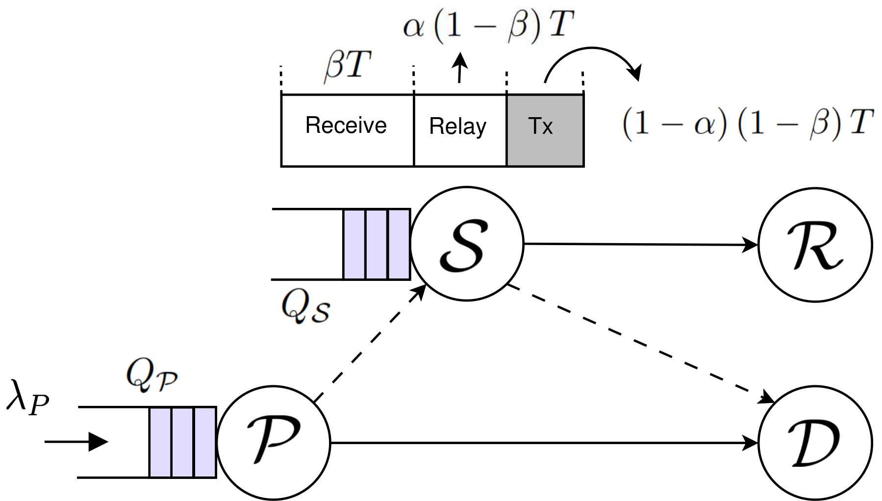
Refer to caption — Fig. 1: System model of SU relaying PU packets and transmitting own packets using two-phase relaying and time sharing

II-A Queue blocking and packet loss

Packet arrival process at PU queue $Q_{\mathcal{P}}$ is Bernoulli with average rate $\lambda_{P}\in\left[0,\,1\right]$ packets/slot. A packet is removed from $Q_{\mathcal{P}}$ only when it is received at $\mathcal{D}$ or $\mathcal{S}$ . A PU packet is admitted to the relay queue $Q_{\mathcal{S}}$ when all of the following events are true– 1) Packet transmission on $\mathcal{P}-\mathcal{D}$ link fails, 2) PU packet is successfully received at $\mathcal{S}$ , and 3) $Q_{\mathcal{S}}$ is not full. Thus, packet departure rate at $Q_{\mathcal{P}}$ , denoted as $\mu_{P}$ , depends on channel between $\mathcal{P}-\mathcal{S}$ and state of $Q_{\mathcal{S}}$ . When $Q_{\mathcal{P}}$ is full, new packets cannot be admitted to the queue and are dropped.

PU queue can be modeled as a discrete time Markov chain (DTMC) as shown in Fig 2(a) where states denote number of packets in PU queue. Let $w_{n},\,n=0,\,1,\dots,\,N_{P}$ be steady state probability of PU queue being in state $n$ . Also let $\gamma=\frac{\lambda_{P}\left(1-\mu_{P}\right)}{\left(1-\lambda_{P}\right)\mu_{P}}$ . Then we can write local balance equations for DTMC of $Q_{\mathcal{P}}$ as

	$\displaystyle w_{1}$	$\displaystyle=\frac{\gamma}{\left(1-\mu_{P}\right)}w_{0},$		(2)
	$\displaystyle w_{n+1}$	$\displaystyle=\gamma\,w_{n},\,n=1,\,2,\dots,\,N_{P}-1.$		(3)

Noting that $w_{n}=\gamma^{n-1}w_{1},\,n>1$ and $\sum_{n=0}^{N_{P}}w_{n}=1$ , we get probability of $Q_{\mathcal{P}}$ being empty as

w_{0}=\begin{cases}\frac{\left(1-\mu_{P}\right)\left(1-\gamma\right)}{1-\mu_{P}\left(1-\gamma\right)-\gamma^{N_{P}+1}}&\,\,\mbox{for}\,\,\gamma\neq 1\\ \frac{1-\mu_{P}}{N_{P}+1-\mu_{P}}&\,\,\mbox{for}\,\,\gamma=1.\end{cases}

Then probabilities of $Q_{\mathcal{P}}$ being non-empty and $Q_{\mathcal{P}}$ being full are given by $\nu_{1}=1-w_{0}$ and $\nu_{N_{P}}=w_{N_{P}}=\frac{1}{\left(1-\mu_{P}\right)}\gamma^{N_{P}}w_{0}$ respectively. To keep PU packet loss below a limit, probability of $Q_{\mathcal{P}}$ being full should remain below a threshold $\epsilon$ , i.e. $\nu_{N_{P}}\leq\epsilon$ . From Fig. 2(a), we observe that, any increase in $\mu_{P}$ would decrease probability of $Q_{\mathcal{P}}$ being full, that is, $\nu_{N_{P}}$ monotonically decreases in $\mu_{P}$ . Thus, for given value of $\lambda_{P}$ , we can find $\overline{\mu_{P}}\in\left[0,\,1\right]$ such that $\nu_{N_{P}}\left(\overline{\mu_{P}}\right)=\epsilon$ , using Bisection method. Packet loss constraint $\nu_{N_{P}}\leq\epsilon$ can now be written as $\mu_{P}\geq\overline{\mu_{P}}$ . SU should choose its access probability in such a way that packet loss constraint of PU is satisfied.

III Optimal spectrum access

DTMC of the relay queue $Q_{\mathcal{S}}$ is as shown in Fig. 2(b) where state $n$ denotes number of packets in relay queue at the end of receiving phase. Probability of a PU packet arriving at $Q_{\mathcal{S}}$ is $q$ . When $Q_{\mathcal{S}}$ is in state $n$ , SU transmits its own packets with probability $p_{n}$ using time sharing. Thus, with probability $\left(1-p_{n}\right)$ , PU packet is relayed for duration $\left(1-\beta\right)T$ and with probability $p_{n}$ , PU packet is relayed for duration $\alpha\left(1-\beta\right)T$ . Then probability of a PU packet departing $Q_{\mathcal{S}}$ in state $n>0$ is

r_{n}=\left(1-p_{n}\right)\theta_{\mathcal{SD}}+p_{n}\overline{\theta_{\mathcal{SD}}}=\theta_{\mathcal{SD}}-p_{n}\left(\theta_{\mathcal{SD}}-\overline{\theta_{\mathcal{SD}}}\right).

(4)

When PU is present, a packet is received at $\mathcal{S}$ with probability $\left(1-\theta_{\mathcal{PD}}\right)\theta_{\mathcal{PS}}$ . Thus, we have $q=\nu_{1}\theta_{\mathcal{PS}}\left(1-\theta_{\mathcal{PD}}\right)$ . For $1\leq n<N_{S}$ , state transition from $n$ to $\left(n+1\right)$ occurs when packet transmission of a packet in $Q_{\mathcal{S}}$ fails and a new PU packet is received, which happens with probability $q\left(1-r_{n}\right)$ . State transition from $n$ to $\left(n-1\right)$ occurs when a packet is successfully relayed and no new packet arrives, which happens with probability $\left(1-q\right)r_{n}$ . Let $\pi_{n},\,n=0,\,1,\dots,\,N_{S}$ be steady state probability of $Q_{\mathcal{S}}$ being in state $n$ . Then we write local balance equations as

	$\displaystyle\pi_{1}$	$\displaystyle=\frac{q}{\left(1-q\right)r_{1}}\pi_{0},$		(5)
	$\displaystyle\pi_{n+1}$	$\displaystyle=\frac{q\left(1-r_{n}\right)}{\left(1-q\right)r_{n+1}}\pi_{n},\,\,n=1,\,2,\dots,\,N_{S}-1.$		(6)

For given values of $\lambda_{P}$ and $\mu_{P}$ , steady state probabilities of relay queue can be calculated from (5), (6) using

\sum_{n=0}^{N_{S}}\pi_{n}=1.

(7)

At the start of receiving phase, $Q_{\mathcal{S}}$ is full with probability $\pi_{N_{S}}\left(1-r_{N_{S}}\right)$ . As a PU packet is admitted to $Q_{\mathcal{S}}$ only when $Q_{\mathcal{S}}$ is not full, we obtain packet departure rate of PU queue as

\mu_{P}=\theta_{\mathcal{PD}}+\theta_{\mathcal{PS}}\left(1-\theta_{\mathcal{PD}}\right)\left[1-\pi_{N_{S}}\left(1-r_{N_{S}}\right)\right].

(8)

III-A SU throughput maximization

When there are $n>0$ packets in $Q_{\mathcal{S}}$ , SU transmits its own packet for duration $\left(1-\alpha\right)\left(1-\beta\right)T$ with probability $p_{n}$ . If $Q_{\mathcal{S}}$ is empty, whole duration $\left(1-\beta\right)T$ is used to transmit SU packet with probability $p_{0}=1$ . Given PU packet arrival rate $\lambda_{P}$ , our objective is to maximize SU packet throughput while ensuring that packet loss probability of PU is kept below specified threshold. Thus, the optimization problem is written as

$\displaystyle\max_{\boldsymbol{p},\,\boldsymbol{\pi},\,\mu_{P}}$	$\displaystyle\quad\mu_{S}=\theta_{\mathcal{SR}}\pi_{0}+\overline{\theta_{\mathcal{SR}}}\sum_{n=1}^{N_{S}}\pi_{n}p_{n}$	(9)
s. t.	$\displaystyle\quad\mu_{P}\geq\overline{\mu_{P}},$	(10)
	$\displaystyle\quad 0\leq p_{n},\pi_{n}\leq 1,\,\,n=0,\,1,\dots,\,N_{S},$
	$\displaystyle\quad p_{0}=1$
	$\displaystyle\quad\mu_{P}=\theta_{\mathcal{PD}}+\theta_{\mathcal{PS}}\left(1-\theta_{\mathcal{PD}}\right)\left[1-\pi_{N_{S}}\left(1-r_{N_{S}}\right)\right],$
	$\displaystyle\quad(\ref{eq:balance1}),\,(\ref{eq:balance2}),\,(\ref{eq:normalize}),$

where $\boldsymbol{p}=\left[p_{0},\dots,\,p_{N_{S}}\right]^{T}$ and $\boldsymbol{\pi}=\left[\pi_{0},\dots,\,\pi_{N_{S}}\right]^{T}$ . Optimization problem in (9) is non-convex due to product terms of optimization variables $\pi_{n}$ and $p_{n}$ . We transform it into a linear programming (LP) problem by exploiting structure of the problem.

Let $a_{n}=\pi_{n}p_{n}$ . Then we have $a_{0}=\pi_{0}$ and $0\leq a_{n}\leq\pi_{n},\,\,n=1,\,2,\dots,\,N_{S}$ . From (7), we have

0\leq\sum_{n=0}^{N_{S}}a_{n}\leq 1.

(11)

Using (4), we can transform balance equations (5) and (6) as given in (12) and (13) on next page.

\theta_{\mathcal{SD}}\left(1-q\right)\pi_{1}-q\pi_{0}=\left(\theta_{\mathcal{SD}}-\overline{\theta_{\mathcal{SD}}}\right)\left(1-q\right)a_{1},

(12)

\theta_{\mathcal{SD}}\left(1-q\right)\pi_{n+1}-q\left(1-\theta_{\mathcal{SD}}\right)\pi_{n}=\left(\theta_{\mathcal{SD}}-\overline{\theta_{\mathcal{SD}}}\right)\left(1-q\right)a_{n+1}+q\left(\theta_{\mathcal{SD}}-\overline{\theta_{\mathcal{SD}}}\right)a_{n},\,\,n=1,\dots,\,N_{S}-1.

(13)

Similarly, constraint in (8) can be written as

\left(1-\theta_{\mathcal{SD}}\right)\pi_{N_{S}}+\left(\theta_{\mathcal{SD}}-\overline{\theta_{\mathcal{SD}}}\right)a_{N_{S}}=1-\frac{\mu_{P}-\theta_{\mathcal{PD}}}{\theta_{\mathcal{PS}}\left(1-\theta_{\mathcal{PD}}\right)}.

(14)

Thus, constraints (5), (6), (8) are transformed into constraints (11), (12), (13) and (14) which are affine in $\pi_{n}$ and $a_{n}$ . The optimization problem in (9) is still non-convex in $\mu_{P}$ . However, for a given value of $\mu_{P}$ , the problem becomes a LP problem in variables $\boldsymbol{\pi}$ and $\boldsymbol{a}=\left[a_{0},\,a_{1},\dots,\,a_{N_{S}}\right]^{T}$ and is written as

$\displaystyle\max_{\boldsymbol{\pi},\,\boldsymbol{a}}$	$\displaystyle\quad\theta_{\mathcal{SR}}a_{0}+\overline{\theta_{\mathcal{SR}}}\sum_{n=1}^{N_{S}}a_{n}$	(15)
s. t.	$\displaystyle\quad 0\leq\pi_{n}\leq 1,\,\,n=0,\thinspace 1,\dots,\,N_{S},$
	$\displaystyle\quad a_{0}=\pi_{0},\,\,0\leq a_{n}\leq\pi_{n},\,\,n=1,\,2,\dots,\,N_{S},$
	$\displaystyle\quad(\ref{eq:normalize}),\,(\ref{eq:normalize_new}),\,(\ref{eq:balance_new_1}),\,(\ref{eq:balance_new_2}),\,(\ref{eq:mup_relay_new}).$

From (8) and (10), we see that the feasible values of $\mu_{P}$ are

	$\displaystyle\max\left\{\overline{\mu_{P}},\,\theta_{\mathcal{PD}}+\theta_{\mathcal{PS}}\overline{\theta_{\mathcal{SD}}}\left(1-\theta_{\mathcal{PD}}\right)\right\}$
		$\displaystyle\hskip-85.35826pt\leq\mu_{P}\leq\theta_{\mathcal{PD}}+\theta_{\mathcal{PS}}\left(1-\theta_{\mathcal{PD}}\right).$		(16)

The linear program in (15) is solved over feasible values of $\mu_{P}$ . Value of $\mu_{P}$ that corresponds to the maximum SU packet throughput is chosen. From optimal $a_{n}$ and $\pi_{n}$ , optimal SU access probabilities are found as $p_{n}=\frac{a_{n}}{\pi_{n}},\,\,n=0,\,1,\dots,\,N_{S}$ . We have used CVX package for MATLAB [14] to solve (15) in polynomial complexity.

III-B Suboptimal methods

From (4), (5), (6) and (7), we get steady state probabilities for $Q_{\mathcal{S}}$ as

	$\displaystyle\pi_{0}$	$\displaystyle=\left[1+\frac{1}{r_{1}}\sum_{n=1}^{N_{S}}\left(\frac{q}{1-q}\right)^{n}\prod_{m=1}^{n-1}\left(\frac{1-r_{m}}{r_{m+1}}\right)\right]^{-1},$		(17)
	$\displaystyle\pi_{n}$	$\displaystyle=\left[\left(\frac{q}{1-q}\right)^{n}\frac{1}{r_{1}}\prod_{m=1}^{n-1}\left(\frac{1-r_{m}}{r_{m+1}}\right)\right]\pi_{0},\,\,n>0.$		(18)

It can be proven that $\pi_{0}$ is monotonically decreasing function of access probability $p_{n},\,n=1,\,2,\dots,\,N_{S}$ . Also we can prove that $\pi_{n},\,0<n\leq N_{S}$ is a monotonically increasing function of $p_{m},\,m\leq n$ and a monotonically decreasing function of $p_{m},\,m>n$ . Intuitively, this can be explained from Fig. 2(b) as follows. As access probability $p_{m}$ increases, packet departure rate of $Q_{\mathcal{S}}$ decreases. Thus, more packets get queued up in $Q_{\mathcal{S}}$ . Hence, the probability of $Q_{\mathcal{S}}$ having more than $m$ packets increases, while probability of $Q_{\mathcal{S}}$ having packets less than or equal to $m$ decreases. Using this nature, we propose low complexity suboptimal methods that simplify $\left(N_{S}+1\right)$ dimensional problem in (9) to a one-dimensional problem.

III-B1 Constant probability transmission (CPT)

In this method, SU transmits its own packets with a fixed probability $p$ when there are $n>0$ packets in relay queue. Thus, we have

p_{n}=\begin{cases}1&\,\mbox{for}\,n=0\\ p&\,\mbox{otherwise}.\end{cases}

(19)

In this case, SU packet throughput is $\mu_{S}=\theta_{\mathcal{SR}}\pi_{0}+\overline{\theta_{\mathcal{SR}}}p\sum_{n=1}^{N_{S}}\pi_{n}$ . Using $\sum_{n=1}^{N_{S}}\pi_{n}=1-\pi_{0}$ , we can write the problem of maximizing $\mu_{S}$ for fixed $\mu_{P}$ as

	$\displaystyle\max_{p\in\left[0,\,1\right]}$	$\displaystyle\quad\overline{\theta_{\mathcal{SR}}}p+\pi_{0}\left(\theta_{\mathcal{SR}}-\overline{\theta_{\mathcal{SR}}}p\right)$
	s. t.	$\displaystyle\quad(\ref{eq:mup_relay}),\,(\ref{eq:balance1}),\,(\ref{eq:balance2}),\,(\ref{eq:normalize}),\,(\ref{eq:prob_const_trans}).$

The term $\pi_{0}\left(\theta_{\mathcal{SR}}-\overline{\theta_{\mathcal{SR}}}p\right)$ is monotonically decreasing in $p$ while term $\overline{\theta_{\mathcal{SR}}}p$ is increasing in $p$ . Thus, there exists a unique $p$ that maximizes $\mu_{S}$ . Optimal solution can be found using Interval halving method with complexity $\mathcal{O}\left(1\right)$ .

III-B2 Step transmission (ST)

In this method, SU transmits its own packets using time sharing with probability $1$ until length of $Q_{\mathcal{S}}$ reaches a threshold $N_{th}$ . Once it crosses $N_{th}$ , the relaying phase duration of $\left(1-\beta\right)T$ is used only to relay PU packets. Thus, we have

p_{n}=\begin{cases}1&\,\mbox{for}\,n\leq N_{th}\\ 0&\,\mbox{otherwise}.\end{cases}

(20)

In this case, the objective is

	$\displaystyle\max_{N_{th}\in\left\{0,\,1,\dots,\,N_{S}\right\}}$	$\displaystyle\quad\theta_{\mathcal{SR}}\pi_{0}+\overline{\theta_{\mathcal{SR}}}\sum_{n=1}^{N_{th}}\pi_{n}$
	s. t.	$\displaystyle\quad(\ref{eq:balance1}),\,(\ref{eq:balance2}),\,(\ref{eq:normalize}),\,(\ref{eq:mup_relay}),\,(\ref{eq:prob_step_trans}).$

With increasing $N_{th}$ , $\pi_{0}$ decreases while number of terms in summation increase. If value of $\overline{\theta_{\mathcal{SR}}}$ is very low compared to $\theta_{\mathcal{SR}}$ , decrease in $\pi_{0}$ is significant and $\mu_{S}$ initially decreases. But as $\pi_{0}$ approaches zero, $\mu_{S}$ increases due to increasing value of $\overline{\theta_{\mathcal{SR}}}\sum_{n=1}^{N_{th}}\pi_{n}$ . For high value of $\overline{\theta_{\mathcal{SR}}}$ , $\mu_{S}$ increases with increasing $N_{th}$ . Throughput drops to zero when $\pi_{N_{S}}$ increases to such a value that constraint (4) cannot be satisfied. Value of $N_{th}$ that maximizes $\mu_{S}$ can be found by linear search with complexity $\mathcal{O}\left(N_{S}\right)$ .

Suboptimal methods run over all feasible values of $\mu_{P}$ given in (16) and the value that corresponds to maximum SU packet throughput is chosen.

IV Numerical results and discussion

Parameter values used to plot results are as follows. Transmit power is $P_{\mathcal{P}}=P_{\mathcal{S}}=0.1\,\mbox{W}.$ Frame duration is $T=100\,\mbox{ms}$ . Time sharing factors are $\beta=\alpha=0.5$ unless stated otherwise. All channels have average channel gain $\sigma_{sd}^{2}=-10\,\mbox{dB},\,s,d\in\left\{\mathcal{P},\,\mathcal{S},\,\mathcal{D},\,\mathcal{R}\right\}$ . Noise power is $\sigma_{\mathcal{N}}^{2}=10^{-5}\,\mbox{W}$ . We take $\mathcal{B}/W=3\times 10^{-3}\,\mbox{bits/Hz}$ . We consider $r_{\mathcal{PS}}=r_{\mathcal{SD}}=r_{\mathcal{SR}}=100\,\mbox{m}$ . Path loss exponent is $\kappa=2$ . Packet loss probability threshold is $\epsilon=0.01$ .

IV-1 Throughput region

Fig. 3: SU packet throughput

\mu_{S}

versus PU packet arrival rate

\lambda_{P}

for

N_{S}=10

and

N_{P}\rightarrow\infty

Fig. 3 plots throughput region of proposed cooperation model. As $\lambda_{P}$ increases, higher $\mu_{P}$ is required to satisfy PU packet loss constraint. To support high $\mu_{P}$ , SU lowers its access probability. Thus, $\mu_{S}$ decreases with increase in $\lambda_{P}$ . As $\lambda_{P}$ increases further, constraint (10) becomes infeasible, at which point $\mu_{S}$ drops to zero. We also see that performance of constant probability transmission (CPT) method and step transmission (ST) method is close to that of optimal method. Hence, the suboptimal methods are good low-complexity alternatives to the optimal method.

As a baseline for comparison, we also plot throughput region of cooperative relaying method (CRM) in [13]. In CRM, PU utilizes whole undivided frame duration $T$ for transmission/reception and optimizes SU access probability under PU queue stability constraint. In contrast, two-phase relaying model dedicates $\beta T$ duration for reception in each slot. Thus, in CRM, probabilities of successful transmission on $\mathcal{P}-\mathcal{D}$ and $\mathcal{S}-\mathcal{R}$ links are higher, resulting in better performance of CRM at low and high values of $\lambda_{P}$ . But in mid-range of $\lambda_{P}$ , two-phase relaying benefits by gaining time to transmit own packets as SU relays PU packets in the same slot.

IV-2 Effect of queue sizes

Fig. 4: Effect of queue sizes on SU packet throughput

\mu_{S}

for (a)

N_{S}=10

(b)

N_{P}=100

and

\lambda_{P}=0.5

Fig. 4(a) plots SU packet throughput $\mu_{S}$ against PU queue capacity $N_{P}$ for different values of $\mathcal{P}-\mathcal{D}$ channel gains. Low values of $N_{P}$ cannot satisfy packet loss constraint in (10). Packet throughput achieved in such infeasible cases in zero. Increasing $N_{P}$ decreases $\overline{\mu_{P}}$ which is the minimum PU departure rate required to satisfy packet loss constraint. This allows SU to transmit its own packets with higher access probabilities. Thus, $\mu_{S}$ increases with increase in $N_{P}$ . As $N_{P}$ increases further, decrease in $\overline{\mu_{P}}$ is insignificant. Access probabilities of SU become constant and in turn $\mu_{S}$ becomes constant. For high value of $\sigma_{\mathcal{PD}}^{2}$ , PU packet arrival rate at $Q_{\mathcal{S}}$ is less which allows higher SU access probabilities. Thus, $\mu_{S}$ increases as $\sigma_{\mathcal{PD}}^{2}$ increases.

Fig. 4(b) shows an interesting tradeoff involving relay queue capacity $N_{S}$ . Increase in $N_{S}$ allows SU to transmit its own packets with higher probability. Also, from (17), we observe that increase in $N_{S}$ decreases probability of relay queue being empty $\pi_{0}$ . For high values of $\sigma_{\mathcal{PD}}^{2}$ , PU packet arrival rate at $Q_{\mathcal{S}}$ is less. In this case, decrease in $\pi_{0}$ (and subsequent decrease in $\theta_{\mathcal{SR}}\pi_{0}$ ) is significant compared to increase in $\mu_{S}$ due to higher access probability. Thus, $\mu_{S}$ decreases with increase in $N_{S}$ . For low values of $\sigma_{\mathcal{PD}}^{2}$ , PU packet arrival rate at $Q_{\mathcal{S}}$ is more. In this case, increase in SU throughput due to higher access probability is significant. But as $N_{S}$ increases further, $\pi_{0}$ approaches zero and $\sum_{n=1}^{N_{S}}\pi_{n}p_{n}$ decreases. Thus, with increasing $N_{S}$ , $\mu_{S}$ initially increases and then gradually decreases.

IV-3 Effect of distance

Fig. 5: Effect of distance between PU source and relay

r_{\mathcal{PS}}

on SU packet throughput

\mu_{S}

for

N_{P}=100

N_{S}=10

\lambda_{P}=0.5

and

r_{\mathcal{PD}}=200\,\mbox{m}

Fig. 5 plots SU throughput against distance between PU source and SU source $r_{\mathcal{PS}}$ . Here, we assume that $\mathcal{D}$ and $\mathcal{R}$ are in close vicinity and lie on the line connecting $\mathcal{P}$ and $\mathcal{S}$ . Then for given $r_{\mathcal{PD}}$ , we have $r_{\mathcal{SD}}=r_{\mathcal{SR}}=r_{\mathcal{PD}}-r_{\mathcal{PS}}$ . When $\mathcal{P}-\mathcal{D}$ channel is weak, PU packet arrival rate at SU is high. Thus, probability of $Q_{\mathcal{S}}$ being full is high. As SU moves away from PU source, $\theta_{\mathcal{PS}}$ decreases, while $\theta_{\mathcal{SD}}$ , $\theta_{\mathcal{SR}}$ , $\overline{\theta_{\mathcal{SD}}}$ and $\overline{\theta_{\mathcal{SR}}}$ increase. This increases SU throughput. As $r_{\mathcal{PS}}$ increases further, $\mu_{P}$ decreases to such a point that queue blocking constraint cannot be satisfied for given $\lambda_{P}$ . In this infeasible region, $\mu_{S}$ is zero. When $\mathcal{P}-\mathcal{D}$ channel is strong, decrease in $\mu_{P}$ due to increasing $r_{\mathcal{PS}}$ is insignificant. Thus, SU throughput $\mu_{S}$ keeps increasing as $\mathcal{S}$ moves closer to $\mathcal{R}$ .

IV-4 Effect of time sharing

Fig. 6 plots $\mu_{S}$ against time sharing factors $\beta$ and $\alpha$ . When $\beta$ is low, values of $\theta_{\mathcal{PD}}$ and $\theta_{\mathcal{PS}}$ are low. This results in lower value of $\mu_{P}$ that cannot support given $\lambda_{P}$ . As $\beta$ increases, PU packet departure rate increases. This allows SU to transmit its own packets with non-zero probability. Thus, $\mu_{S}$ increases. As $\beta$ increases further, less time is available for SU to transmit its own packets which decreases $\theta_{\mathcal{SR}}$ . Thus, $\mu_{S}$ decreases at high value of $\beta$ . As $\alpha$ increases, $\overline{\theta_{\mathcal{SD}}}$ increases while $\overline{\theta_{\mathcal{SR}}}$ decreases. Increase in departure rate of PU packets from $Q_{\mathcal{S}}$ allows SU to transmit its own packet with higher access probability. Thus, $\mu_{S}$ increases with increasing $\alpha$ . But as $\alpha$ increases further, decrease in $\overline{\theta_{\mathcal{SR}}}$ becomes dominant, in turn decreasing $\mu_{S}$ . This indicates that there is scope to improve $\mu_{S}$ by optimizing $\beta$ and $\alpha$ . However, the problem is difficult to solve as objective in (9) is non-convex in $\beta$ and $\alpha$ .

V Conclusion

We studied a CR system where SU employs two-phase relaying to relay failed PU packets. Both users have packet queues of finite capacity which results in packet loss. We proposed optimal as well as suboptimal access methods for SU to maximize its packet throughput under packet loss constraint of PU. We observed that two-phase relaying model performs better than cooperation model without time sharing for mid-range values of PU packet arrival rate. Suboptimal methods have negligible loss in the performance and are good low complexity alternatives to the optimal method. Furthermore, results revealed that as relay queue size increases, SU throughput improves initially but then decreases. PU queue size limits maximum supported PU packet arrival rate.

References

[1] O. Simeone, Y. Bar-Ness, and U. Spagnolini, “Stable throughput of cognitive radios with and without relaying capability,” IEEE Trans. Commun., vol. 55, no. 12, pp. 2351–2360, 2007.
[2] J. Jeon and A. Ephremides, “The stability region of random multiple access under stochastic energy harvesting,” in Proc. IEEE Int. Symp. Inf. Theory (ISIT), St. Petersburg, Russia, July 2011, pp. 1796–1800.
[3] A. Fanous and A. Ephremides, “Stable throughput in a cognitive wireless network,” IEEE J. Sel. Areas Commun., vol. 31, no. 3, pp. 523–533, 2013.
[4] S. Kompella, G. Nguyen, C. Kam, J. Wieselthier, and A. Ephremides, “Cooperation in cognitive underlay networks: Stable throughput tradeoffs,” IEEE/ACM Trans. Netw., vol. PP, no. 99, pp. 1756–1768, 2013.
[5] M. Ashour, A. Elsherif, T. Elbatt, and A. Mohamed, “Cognitive radio networks with probabilistic relaying: Stable throughput and delay tradeoffs,” IEEE Trans. Commun., vol. PP, no. 99, pp. 4002–4014, 2015.
[6] T. M. C. Chu, H. Phan, and H. Zepernick, “On the performance of underlay cognitive radio networks using M/G/1/K queueing model,” IEEE Commun. Lett., vol. 17, no. 5, pp. 876–879, May 2013.
[7] I. Krikidis, T. Charalambous, and J. S. Thompson, “Buffer-aided relay selection for cooperative diversity systems without delay constraints,” IEEE Trans. Wireless Commun., vol. 11, no. 5, pp. 1957–1967, May 2012.
[8] A. Ikhlef, D. S. Michalopoulos, and R. Schober, “Max-max relay selection for relays with buffers,” IEEE Trans. Wireless Commun., vol. 11, no. 3, pp. 1124–1135, March 2012.
[9] N. Zlatanov, R. Schober, and P. Popovski, “Buffer-aided relaying with adaptive link selection,” IEEE J. Sel. Areas Commun., vol. 31, no. 8, pp. 1530–1542, August 2013.
[10] S. Luo and K. C. Teh, “Buffer state based relay selection for buffer-aided cooperative relaying systems,” IEEE Trans. Wireless Commun., vol. 14, no. 10, pp. 5430–5439, Oct 2015.
[11] N. Nomikos, T. Charalambous, I. Krikidis, D. N. Skoutas, D. Vouyioukas, M. Johansson, and C. Skianis, “A survey on buffer-aided relay selection,” IEEE Commun. Surveys Tuts., vol. 18, no. 2, pp. 1073–1097, Second quarter 2016.
[12] A. El Shafie, M. Khafagy, and A. Sultan, “Optimization of a relay-assisted link with buffer state information at the source,” IEEE Commun. Lett., vol. 18, no. 12, pp. 2149–2152, Dec 2014.
[13] A. Elmahdy, A. El-Keyi, T. Elbatt, and K. Seddik, “On the stable throughput of cooperative cognitive radio networks with finite relaying buffer,” in Proc. IEEE 25th Int. Symp. Personal, Indoor, and Mobile Radio Commun. (PIMRC 2014), Washington DC, USA, Sept 2014, pp. 942–946.
[14] M. Grant and S. Boyd, “CVX: Matlab software for disciplined convex programming, version 2.1,” http://cvxr.com/cvx, Mar. 2014.