Supplement to : “On optimality of sliced inverse regression in high dimensions”
Abstract
The central subspace of a pair of random variables is the minimal subspace such that . In this paper, we consider the minimax rate of estimating the central space of the multiple index models with at most active predictors where . We first introduce a large class of models depending on the smallest non-zero eigenvalue of , over which we show that an aggregated estimator based on the SIR procedure converges at rate . We then show that this rate is optimal in two scenarios: the single index models; and the multiple index models with fixed central dimension and fixed . By assuming a technical conjecture, we can show that this rate is also optimal for multiple index models with bounded dimension of the central space. We believe that these (conditional) optimal rate results bring us meaningful insights of general SDR problems in high dimensions.
Keywords:
semi-definite positive programming,keywords
journalname
t1Lin’s research is supported by the Center of Mathematical Sciences and Applications at Harvard University. Liu’s research is supported by the NSF Grant DMS-1120368 and NIH Grant R01 GM113242-01
and
1 Introduction
Because of rapid advances of information technologies in recent years, it has become a common problem for data analysts that the dimension () of data is much larger than the sample size (), i.e., the ‘large , small problem’. For these problems, variable selection and dimension reductions are often indispensable first steps. In early 1990s, a fascinating supervised dimension reduction method, the sliced inverse regression (SIR) (Li, 1991), was proposed to model univariate response with a low dimensional projection of the predictors. More precisely, SIR postulates the following multiple index model for the data:
| (1) |
and estimates the subspace via an eigen-analysis of the estimated conditional covariance matrix . Note that the individual ’s are not identifiable, but the space can be estimated well. Based on the observation that , Cook (1998) proposed a more general framework for dimension reduction without loss of information, often referred to as the Sufficient Dimension Reduction (SDR). Under this framework, researchers look for the minimal subspace such that where is no longer necessarily a scalar response. Although numerous SDR algorithms have been developed in the past decades, SIR is still the most popular one among practitioners because of its simplicity and computational efficiency. Asymptotic theories developed for these SDR algorithms have all focused on scenarios where the data dimension is either fixed or growing at a much slower rate compared with the sample size (Dennis Cook, 2000; Li and Wang, 2007; Li, 2000). The ‘large p, small n’ characteristic of modern data raises new challenges to these SDR algorithms.
Lin et al. (2015) recently showed under mild conditions that the SIR estimate of the central space is consistent if and only if . This provides a theoretical justification for the necessity of the structural assumption such as sparsity for SIR when . A commonly employed and also practically meaningful structural assumption made for high-dimensional linear regression problems is the sparsity assumption, i.e., only a few predictors among the thousands or millions of candidate ones participate in the model. We will show that this sparsity assumption can also rescue the curse of dimension for dimension reduction algorithms such as SIR. Motivated by the Lasso and the regularized sparse PCA (Tibshirani, 1996; Zou and Hastie, 2005), Li and Nachtsheim (2006) and Li (2007) proposed some regularization approaches for SIR and SDR. However, these approaches often fail in high dimensional numerical examples and are difficult to rectify because little is known about theoretical behaviors of these algorithms in high dimensional problems. The DT-SIR algorithm in Lin et al. (2015) and the Sparse-SIR algorithm in Lin et al. (2016b), however, have been shown to provide consistent estimations. We agree with Cook et al. (2012) that a detailed understanding of “the behaviour of these SDR estimators when is not large relative to ” might be the key to efficient high-dimensional SDR algorithms. The main objective of the current paper is to understand the fundamental limits of the sparse SIR problem from a decision theoretic point of view. Such an investigation is not only interesting in its own right, but will also inform the development and evaluation of other SDR algorithms developed for high-dimensional problems.
Neykov et al. (2015) considered the (signed)-support recovery problem of the following class of single index models
where , . Let , they proved that 1) If is sufficiently small, any algorithm fails to recover the (signed) support of with probability at least and 2) If is sufficiently large, the DT-SIR algorithm (see Lin et al. (2015) or Algorithm 1 below) can recover the (signed) support with probability converging to 1 as . That is, the minimal sample size required to recover the support of is of order . These results shed us some light on the possibility of obtaining the optimal rate of SIR-type algorithms in high dimension.
SIR is widely considered as a ‘generalized eigenvector’ problem (Chen and Li, 1998). Inspired by recent advances in sparse PCA (Amini and Wainwright, 2008; Johnstone and Lu, 2004; Cai et al., 2013; Birnbaum et al., 2013; Vu and Lei, 2012), where researchers aim at estimating the principal eigenvectors of the spiked models, it is reasonable to expect a similar phase transition phenomenon (Johnstone and Lu, 2004), the signed support recovery (Amini and Wainwright, 2008), and the optimal rate (Cai et al., 2013) for SIR when . However, as it was pointed out in Lin et al. (2015), the sample means in corresponding slices are neither independent nor identically distributed. The usual concentration inequalities are not applicable. This difficulty forced them to develop the corresponding deviation properties, i.e., the ‘key lemma’ in Lin et al. (2015). On the other hand, the observation that the number of slices is allowed to be finite when is bounded (as we always require that ) suggests that a consistent estimate of the central space based on finite (e.g., ) sample means is possible. This is again similar to the so-called High dimensional low sample size (HDLSS) scenario of PCA, which was first studied in Jung et al. (2009) by estimating the principal eigenvectors based on finite samples. These connections suggest that theoretical issues in sparse SIR might be analogous to those in sparse PCA. However, our results in this article suggest that sparse linear regression is a more appropriate prototype for sparse SIR.
The main contribution of this article is the determination of the minimax rate for estimating the central space over two classes of models and , defined in (8) and (14) respectively. The risk of our interest is , where is an orthogonal matrix formed by an orthonormal basis of , and is an estimate of , the projection matrix associated with the orthogonal matrix . We construct an estimator (computationally unrealistic) such that the risk of this estimator is of order . Under mild conditions, we further demonstrate that the risk of any estimator is bounded below by if the dimension of the central space is bounded. Thus, the minimax rate of the risk is if is bounded. One of the key components of our analysis is the linear algebraic Lemma 16, which might be of independent interest and be used in determining lower bounds of minimax estimation rates for other dimension reduction problems. To the best of our knowledge, this is the first result about the minimax rate of estimating the central space in high dimension. In Subsection 2.6, we show that the computationally efficient algorithm DT-SIR (Lin et al., 2015) achieves this optimal rate when and for some . Furthermore, we investigate the effects of the slice number in the SIR procedure.
The rest of the paper is organized as follows. Section 2 presents the main results of the paper, including the rate of the oracle risk in Section 2.4.1 and the rate of the sparse risk in Section 2.4.2. Since the lower bound can be obtained by modifying some standard arguments, we defer its related proofs to the online supplementary file (Lin et al., 2016a) and give the proofs of upper bounds in Sections 4.1 and 4.2. In Section 5 we discuss potential extensions of our results. More auxiliary results and technical lemmas are included in the online supplementary file (Lin et al., 2016a).
2 Main Results
Since the establishment of the SDR framework about two decades ago, estimating the central space has been investigated under different assumptions (Dennis Cook, 2000; Cook, 1998; Schott, 1994; Ferré, 1998; Li and Wang, 2007; Hsing and Carroll, 1992; Cook et al., 2012). Various SDR algorithms have their own advantages and disadvantages for certain classes of link functions (models). For example, SIR only works when both the linearity and coverage conditions are satisfied (Li, 1991); Sliced Average Variance Estimation (SAVE) (Dennis Cook, 2000) works when the coverage condition is slightly violated but requires the constant variance condition. Thus, to discuss the minimax rate of estimating the central space for model (1), it is necessary to first specify the class of models where one or several algorithms are practically used, and then check if these algorithms and their variants can estimate the central space optimally over this class of models. SIR is one of the most well understood SDR algorithms, and is of special interests to know if it is rate optimal over a large class of models. This will not only improve our understanding of high dimensional behaviors of SIR and its variants, but also bring us insights on behaviors of other SDR algorithms.
2.1 Notation
In addition to those that have been used in Section 1, we adopt the following notations throughout the article. For a matrix , we denote its column space by and its -th row and -th column by and respectively. For vectors and , we denote the -th entry of as and the inner product as . For two positive number a,b, we use and to denote and , respectively. For a matrix , . For a positive integer , denotes the index set . We use , , and to denote generic absolute constants, though the actual value may vary from case to case. For two sequences and , we denote and if there exist positive constants and such that and , respectively. We denote if both and hold.
2.2 A brief review of SIR
Since we are interested in the space spanned by ’s in model (1), without loss of generality, we can assume that is a orthogonal matrix(i.e., ) and the models considered in this paper are
| (2) |
where , , and is the set of all orthogonal matrices. Though is not identifiable, the column space is estimable. The Sliced Inverse Regression (SIR) procedure proposed in Li (1991) estimate the central space without knowing , which can be briefly summarized as follows. Given samples , , SIR first divides them into equal-sized slices according to the order statistics .11 1 To ease notations and arguments, we assume that . We re-express the data as and , where is the double subscript in which refers to the slice number and refers to the order number of a sample in the -th slice, i.e.,
Here is the concomitant of . Let the sample mean in the -th slice be , and the overall sample mean be . SIR estimates by
| (3) |
and estimates the central space by where is the matrix formed by the top eigenvectors of . Throughout this article, we assume that , dimension of the central space, is known.
In order for the SIR to give a consistent estimate of the central space, following sufficient conditions have been suggested (e.g., Li (1991), Hsing and Carroll (1992) and Zhu et al. (2006)):
-
Linearity Condition and Coverage Condition:
where is the -th columns of the orthogonal matrix .
-
Smoothness and Tail conditions on the Central Curve .
Smoothness condition: For and , let be the collection of all the -point partitions of . The central curve satisfies the following conditions:
Tail condition: For some , there exists a non-decreasing function on , such that
| (4) | ||||
As in Lin et al. (2015), where they demonstrated the phase transition phenomenon of SIR in high dimension, we replace Condition (B′) by
-
Modified Smoothness and Tail conditions,
which is all the same as (B′) except that eqn (4) is replaced by
| (5) | ||||
It is easy to see that Condition (B′′) is slightly stronger than Condition (B′). A main advantage of Condition (B′′) is the following proposition proved in Neykov et al. (2015).
Proposition 1.
If Condition B′′ holds, the central curve satisfies the sliced stable condition (defined below) with .
Definition 1.
Let be a random variable. For , let denote all partitions of , such that
A curve is -sliced stable with respect to Y, if there exist positive constants such that for any partition and any , we have
| (6) |
A curve is sliced stable if it is -sliced stable for some positive constant .
Intuitively, implies that the LHS of (6) converges to zero. Definition 1 states that its convergence rate is a power of , although any function of that converges to 0 can be placed before on the RHS of (6). Thus, the sliced stable condition is almost the necessary condition to ensure that the SIR works. A main advantage of the sliced stable condition is that we can easily quantify the deviation properties of the eigenvalues, eigenvectors, and each entries of . This is one of the main technical contributions of Lin et al. (2015). We henceforth assume that the central curve satisfies the sliced stable condition. As shown by Proposition 1, Condition (B′′) ensures the sliced-stable condition.
2.3 The class of functions
Let , then . Let . Since , the sliced stability for implies the sliced stability for and vice verse. Since we have assumed that , the linearity condition holds automatically. The coverage condition, which requires , can be refined as
| (7) |
for some positive constant . Since , we know . In particular, we have where is assumed to be a fixed constant. This coverage condition is commonly adopted in the literature (e.g., Cai et al. (2013) and Gao et al. (2014)) when researchers discuss the dimension reduction problems. The class of functions satisfying the sliced stable condition and coverage condition is of our main interests in this paper. More precisely, we introduce as below.
Definition 2.
Let and . A function belongs to the class , if the following conditions are satisfied.
-
Coverage condition: where .
-
Sliced stable condition: is sliced stable with respect to , where .
It is easy to see that almost all functions that make SIR work belong to for some and .
2.4 Upper bound of the risk
Suppose we have samples generated from a multiple index model with link function and orthogonal matrix , that is, . We are interested in the risk where is an estimate of based on these samples. In this subsection, we provide an upper bound of this risk. All detailed proofs are deferred to Sections 4.1, 4.2, and online supplementary file (Lin et al., 2016a).
2.4.1 Oracle Risk
Here we are interested in estimating the central space over the following class of models parametrized by :
| (8) |
A main result of this article is:
Theorem 1 (An Upper Bound of Oracle Risk).
Assume that is sufficiently small and . We have
| (9) |
In order to establish the upper bound, we consider the estimate , which is a orthogonal matrix forming by the top- eigenvectors of , and show that achieves the rate in Theorem 1.
A result in Lin et al. (2015), which states that
| (10) |
appears to contradict our Theorem 1 here: (i) it does not depend on , the dimension of central subspace; (ii) it does not depend on , the smallest non-zero eigenvalue of ; (iii) it depends on (the number of slices) and seems worse than our upper bound here. The first two differences appear simply because Lin et al. (2015) have assumed that is bounded and the non-zero eigenvalues of are bounded below by some positive constant (i.e., the information about eigenvalues and is absorbed by some constants). The third difference appears because we here are interested in the convergence rate of the SIR estimate of the space rather than the convergence rate of the SIR estimate of the matrix . As they have pointed out, the convergence rate of might be different (slower) than the convergence rate of . More precisely, we have
| (11) |
From the proof of Theorem 1 of Lin et al. (2015), we can easily check that the first term is of rate and the second term is of rate . Since and share the same column space and we are interested in estimating , the convergence rate of the second term in (11) does not matter provided that is a large enough integer. Thus, Theorem 1 does not contradict the convergence result in Lin et al. (2015).
Remark 1.
On the role of . Researchers have claimed that the performance of SIR procedure is not sensitive to the choice of , i.e., can be as large as (Hsing and Carroll, 1992) and can also be a large enough fixed integer when (Duan and Li, 1991). A direct corollary of Theorem 1 is that if is fixed, can be a large enough constant such that is an optimal estimate of . In the SIR literature, researchers care about the eigenvectors of and ignore the eigenvalue information. In this article, we show that the larger the , the more accurate the estimate of the eigenvalues of , and illustrate this phenomenon via numerical simulations in Section 3.1. Taking the eigenvalue information into consideration will bring us more a detailed understanding of SIR.
2.4.2 Upper bound of the risk of sparse SIR
Lin et al. (2015) shows that when dimension is larger than or comparable with the sample size , the SIR estimate of the central space is inconsistent. Thus, structural assumptions such as sparsity are necessary for high dimensional SIR problem.We here impose the weak sparsity on the loading vectors . For a orthogonal matrix (i.e., ), we order the row norms in decreasing order as and define the weak radius of to be
| (12) |
Let be the set of weak sparse orthogonal matrices. Weak -ball is a commonly used condition for sparsity. See, for example, Abramovich et al. (2006) for wavelet estimation and Cai et al. (2012) for sparse co-variance matrix estimation. Furthermore, we need the notion of effective support , which was introduced by Cai et al. (2013). The size of effective support is defined to be where
| (13) |
and denotes the smallest integer no less than . For more detailed discussions of the sparse orthogonal matrices, we refer to Cai et al. (2013).
In this subsection, we are interested in estimating the central space over the following class of high dimensional models parametrized by :
| (14) |
Let . We have the following result:
Theorem 2 (The Upper Bound of Optimal Rates).
Assume that is fixed, , is sufficiently small and . We have
| (15) |
In order to establish the upper bound in Theorem 2, we need to construct an estimator that attains it. Let be the set of all subsets of with size . To ease the notation, we often drop the subscript of below and assume that there are samples. Let us divide the samples randomly into two equal size sets. Let and be the SIR estimates of based on the first and second sets of samples, respectively. Inspired by the idea in Cai et al. (2013), we introduce the following aggregation estimator of .
Aggregation Estimator
For each , we let
| (16) | ||||
and
Our aggregation estimator is defined to be .
2.5 Lower Bound and Minimax Risk
To avoid unnecessary details, we assume that dimension of the central space is bounded in this subsection. The semi-parametric characteristic of multiple index models brings us additional difficulties in determining the lower bound of the minimax rate. Because of our ignorance on the function class , we can only establish the lower bound in two restrictive cases: (i) , the smallest non-zero eigenvalue of , is bounded below by some positive constant; and (ii) single index models where . To the best of our knowledge, even the optimal rate of estimating the central space depending only on , and in high dimensions has never been discussed in the literature. Furthermore, we have observed from extensive numerical studies that the -th direction is difficult to detect for even with the sample size greater than . This observation conforms to the existing numerical studies reported in the literature, i.e., most researchers only reported numerical studies for models with except that Ferré (1998) performed a numerical study for a model with and reported that the -th direction was hard to discover. Thus, the optimal rate with bounded might be a more reasonable target to pursue.
2.5.1 is bounded below by some positive constant
Assume that , the smallest non-zero eigenvalues of , is bounded below by a positive constant. We have the following optimal convergence rate of the Oracle Risk.
Theorem 3 ( Oracle Risk).
Assume that are bounded. We have
| (18) |
Remark 2.
Although we have assumed that the dimension of the central space is bounded, we include it in the convergence rate to emphasize that the result holds for multiple index models.
Because of Theorem 1, we only need to establish the lower bound. We defer the detailed proof to the online supplementary file (Lin et al., 2016a) and briefly sketch its key steps here. One of the key steps in obtaining the lower bound is constructing a finite family of distributions that are distant from each other in the parameter space and close to each other in terms of the KL-divergence. Recall that, for any sufficiently small and any positive constant , Cai et al. (2013) have constructed a subset , the Grassmannian manifold consisting of all the dimensional subspaces in , such that
for some absolute constants and . For any , if we can choose a orthogonal matrix such that the column space of corresponds to , we may consider the following finite class of models
where is a -variates function with bounded first derivative such that these models belong to . Let denote the joint density of . Simple calculation shows that
| (19) |
If we have
| (20) |
we may apply the standard Fano type argument ( e.g., Cai et al. (2013) ) to obtain the essential rate of the lower bound.
However, (20) is not always true (e.g., it fails if and are two different orthogonal matrices sharing the same column space). We need to carefully specify for each such that they satisfy the inequality (20). It seems to be a simple linear algebraic problem, however, its proof requires (slightly) non-trivial work in differential geometry (cf. Lemma 16). 22 2 Q. Lin appreciates the helpful discussions with Dr. Long Jin Thus we know that the rate in Theorem 1 is optimal if and are bounded. Once the ‘Oracle risk’ has been established, the standard argument in Cai et al. (2013) leads us the following:
Theorem 4 (Optimal Rates ).
Assume that , are bounded, and . We have
| (21) |
Proof.
See the online supplementary file (Lin et al., 2016a).
2.5.2 Single Index Models
If we restrict our consideration to single index models (i.e., ), we have a convergence rate optimally depending on , , , and .
Theorem 5 (Oracle Risk for Single Index Models).
Assuming that and , we have
| (22) |
Since we have proved Theorem 2, all we need to do is to establish a suitable lower bound. Let us consider the following linear model:
where is a unit vector, and . Simple calculation shows that
Thus, inequality (19) becomes
| (23) |
and the desired lower bound follows from the same argument as that of Theorem 3. Once the oracle risk has been established, the standard argument in Cai et al. (2013) leads us to the following result:
Theorem 6 (Optimal Rates : ).
Assume that and . We have
| (24) |
Proof.
It is similar to the proof of Theorem 4 and thus omitted.
2.5.3 Multiple Index Models with bounded
The arguments in the subsection 2.5.2 motivate us to propose the following (conjectural) property for the function class .
Conjecture 1.
If is bounded, there is a constant such that for any , there exists a -variate function such that and
| (25) |
Remark 3.
Inequality (25) can be relaxed to that holds with high probability when .
The construction in subsection 2.5.2 shows that this conjecture holds for . For any , suppose that there exists a function such that . We expect that, for , there exist constants and such that
Note that the density function of is the convolution of the density functions of and . Heuristically, if is (nearly) normal, by the continuity of the convolution operator, we expect that . Since we cannot prove it rigorously, we present some supporting numerical evidences here in Subsection 3.2. Assuming this conjecture, we have the following theorems, of which the proofs are similar to those of Theorem 3 and Theorem 4.
2.6 Optimality of DT-SIR
In the previous section, we have proved that the aggregation estimator is rate optimal. In practice, however, it is computationally too expensive. The DT-SIR algorithm proposed in Lin et al. (2015) is computationally efficient in general, and can be further simplified when .
In this section, we focus on the single index model. with the exact sparsity on the loading vector , i.e., .
Theorem 9.
Suppose for some , is sufficiently small and for some constant . Let be the DT-SIR estimate with threshold level for some constant , then we have
| (28) |
with probability at least for some positive constants and .
Proof.
See the online supplementary file (Lin et al., 2016a).
From Theorem 9, it is easy to see that, if , the DT-SIR estimator is rate optimal. Since there is a computational barrier for the rate optimal estimate of sparse PCA (Berthet and Rigollet, 2013), the fact that the computationally efficient DT-SIR algorithm achieves the optimal rate suggests that sparse PCA might not be an appropriate prototype of SIR in high dimensions.
3 Numerical Studies
In this section, we illustrate three aspects of the high dimensional behavior of SIR via numerical experiments. The first experiment focuses on the impacts of the choice of in SIR: the larger the , the more accurate the estimate of eigenvalue of . The second experiment aims at providing supporting evidence of Conjecture 1. The third experiment demonstrates empirical performances of the DT-SIR algorithm.
3.1 Effects of
Our numerical results below show that the accuracy of estimating the eigenvalues of depends on the choice of . Let us consider the following linear model:33 3 Up to a monotone transform, this is the only case that we can give the explicit value of .
| Model : | (29) |
It is easy to see that the only non-zero eigenvalue of is . The results are shown in Table 1, where ranges in , in and in . Each entry is the empirical mean (standard deviation), calculated based on 100 replications, of the SIR estimate of for given , and .
| 0.319 | 0.446 | 0.479 | 0.503 | 0.509 | 0.520 | 0.551 | ||
| (0.013) | (0.017) | (0.017) | (0.016) | (0.017) | (0.018) | (0.017) | ||
| 0.318 | 0.448 | 0.480 | 0.500 | 0.505 | 0.510 | 0.525 | ||
| (0.009) | ( 0.012) | ( 0.012) | ( 0.012) | ( 0.012) | ( 0.013) | ( 0.012) | ||
| 0.319 | 0.448 | 0.479 | 0.498 | 0.500 | 0.501 | 0.504 | ||
| (0.004) | (0.006) | (0.005) | (0.006) | (0.005) | (0.006) | (0.006) | ||
| 0.319 | 0.448 | 0.479 | 0.498 | 0.499 | 0.501 | 0.503 | ||
| (0.003) | ( 0.004) | (0.004) | (0.004) | (0.004) | (0.004) | (0.004) | ||
| 0.190 | 0.271 | 0.288 | 0.307 | 0.313 | 0.328 | 0.371 | ||
| (0.011) | (0.012) | (0.014) | (0.015) | (0.015) | (0.014) | (0.016) | ||
| 0.191 | 0.27 | 0.288 | 0.302 | 0.307 | 0.312 | 0.335 | ||
| (0.008) | (0.009) | (0.010) | (0.010) | (0.010) | (0.010) | (0.012) | ||
| 0.191 | 0.269 | 0.288 | 0.299 | 0.3 | 0.302 | 0.307 | ||
| (0.003) | (0.004) | (0.005) | (0.005) | (0.005) | (0.005) | ( 0.004) | ||
| 0.191 | 0.269 | 0.288 | 0.299 | 0.3 | 0.301 | 0.303 | ||
| (0.002) | (0.003) | (0.003) | ( 0.004) | ( 0.003) | ( 0.003) | ( 0.003) | ||
| 0.064 | 0.091 | 0.098 | 0.109 | 0.117 | 0.136 | 0.190 | ||
| (0.007) | (0.008) | (0.009) | (0.009) | (0.009) | (0.010) | (0.010) | ||
| 0.0643 | 0.0901 | 0.0973 | 0.103 | 0.108 | 0.117 | 0.144 | ||
| (0.005) | (0.006) | (0.006) | (0.006) | (0.006) | (0.006 ) | (0.007) | ||
| 0.0638 | 0.0899 | 0.0963 | 0.101 | 0.101 | 0.103 | 0.109 | ||
| (0.002) | ( 0.003) | ( 0.003) | ( 0.003) | ( 0.003) | ( 0.003) | ( 0.003) | ||
| 0.0636 | 0.0898 | 0.0961 | 0.100 | 0.100 | 0.102 | 0.104 | ||
| ( 0.001) | ( 0.002) | ( 0.002) | ( 0.002) | ( 0.002) | ( 0.002) | ( 0.002) |
From Table 1, it is clear that the larger the is, the more accurate estimation of the eigenvalue is. Cautious reader may notice that, in the row with and , the empirical mean and the standard error are not behaving as we have expected, e.g., when , the empirical mean and standard error are 0.190 and 0.010, respectively, which are worse than the case with (or ). This is not contradicting our theory. Note that in the Lemma 1, the deviation property of depends on the value , i.e., the larger the is, the more concentrated the is. In particular, for the entry corresponding to , and , the value is much smaller than the corresponding value, 5, associated with the entry with , and .
3.2 Support Evidences of Conjecture 1
Let us consider the following model with two indexes:
| Model : | (30) |
where is a smooth function such that for a small constant ,
| (31) |
and for some constant . Let and be the two eigenvalues of . Since we know that the absolute value of the derivative of the link function , we want to check if holds for some positive constant and and if model (30) belongs to . We study the boundedness of and via numerical simulation. In the simulation, we choose to be 20. Let range in and range in .
| 0.3358 | 0.5969 | 1.6333 | 2.1297 | 4.5681 | 7.1434 | 30.6206 | ||
| 0.3276 | 0.5676 | 1.4416 | 1.7627 | 2.1511 | 2.3908 | 4.3137 | ||
| 0.3272 | 0.5650 | 1.4153 | 1.7092 | 1.9662 | 2.0006 | 2.2554 | ||
| 0.3268 | 0.5651 | 1.4125 | 1.7052 | 1.9465 | 1.9695 | 1.9780 | ||
| 0.1068 | 0.1436 | 0.3227 | 0.5381 | 2.3159 | 4.2023 | 19.5854 | ||
| 0.0899 | 0.1087 | 0.1248 | 0.1206 | 0.2701 | 0.5061 | 2.3384 | ||
| 0.0899 | 0.1059 | 0.1014 | 0.0840 | 0.0462 | 0.0620 | 0.2366 | ||
| 0.0898 | 0.1063 | 0.1001 | 0.0795 | 0.0297 | 0.0190 | 0.0278 |
In Table 2, each entry is the average of 100 replications. For fixed , the larger , the more accurate estimation of In particular, it is easy to see from the row with that are bounded. The row with seems to be contradicting to our conjecture 1, where might be diverging as . This is actually not a contradiction, since we know that the deviation property of depends on the product from Lemma 1. Thus, to get accurate estimate of , we require more samples if is small.
3.3 Performance of DT-SIR
In this section, we assume the exact sparsity for some , and consider the following data generating models,
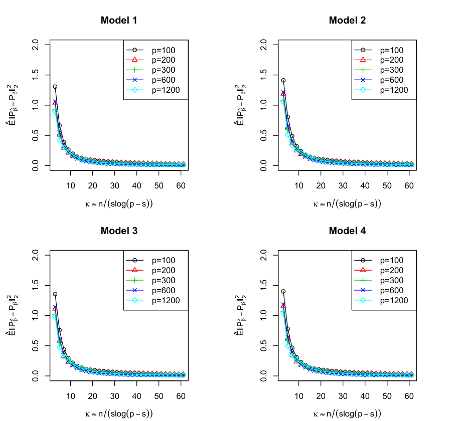
where , , , and is a fixed vector with nonzero coordinates. Let . The dimension of the predictors takes value in , the sparsity parameter is fixed at , and takes values in . For each combination, , , and we simulate data from each model 1000 times. We then get the estimate using DT-SIR algorithm, and the results of the average values of for each model with each combination are shown in Figure 1, which shows the distance between the estimated projection matrix and the true one becomes smaller as increases for all fixed .
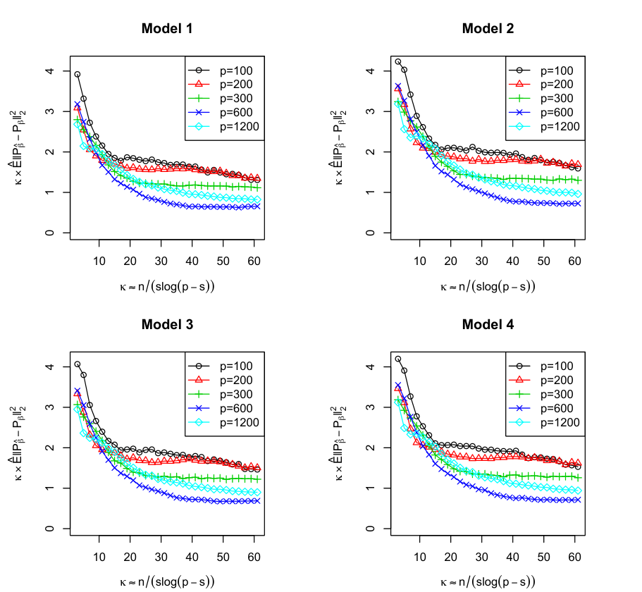
According to Theorem 9, is less than a constant with high probability. Therefore, we also the average values of for these models in Figure 2, which demonstrates that is a decreasing function of and tends to be stable when becomes large enough. These empirical results also validate Theorem 9.
4 Proofs
We need the following technical lemma, which is a direct corollary of the ‘key lemma’ in Lin et al. (2015) :
Lemma 1.
Assume that in the model (2). Let be the SIR estimate (3) of . There exist positive absolute constants , and such that, for any and any , if for sufficiently large constant , then for any unit vector that lies in the column space of , we have
| (32) |
with probability at most
In particularly, if and are bounded, we can choose to be a large enough finite integer such that (32) holds with high probability.
Proof.
It is a direct corollary of the ‘key lamma’ in Lin et al. (2015).
4.1 Proof of Theorem 1
Suppose that we have samples from the distribution defined by the model . Let where is a sufficiently large integer and where is the eigen-vector associated to the -th largest eigen-value of . We introduce the following decomposition
i.e., lies in the central space and lies in the space which is perpendicular to . Let be a orthogonal matrix such that . Since and , we may write for some . Thus we know that . We introduce the notation , , and similar to the definition of . Let , , be three matrices formed by the vectors , , and . We have the following decomposition
| (33) | ||||
where we define and use the fact . Since , we know that the entries of are samples of . First, we have the following lemma.
Lemma 2.
Let . Assume that is sufficiently small. We have the following statements.
- i)
There exist constants and such that
- ii)
For any vector and any , let . Recall that . If we choose sufficiently large such that for some positive constant , there exist positive constants , …, and such that
- iii)
For any , there exist positive constants ,…, and , such that
Let where , , .
Corollary 1.
Lemma 2 implies the following simple results where stands for some absolute constant which might be varying in different statements.
-
If , we have .
-
Conditioning on , we have .
-
Conditioning on , if is sufficiently small, we have .
-
Conditioning on , If is sufficiently small, we have .
Now we start the proof of Theorem 1. Note that
For
It is easy to see that
For
Let be the spectral decomposition of , where is a orthogonal matrix and is a diagonal matrix. Conditioning on , we know that and are sharing the same column space. Thus we have . Let us apply the Sin-Theta theorem (e.g., Lemma 20) to the pair of symmetric matrices ) where . Since is sufficiently small, conditioning on , we have and . Thus, we have
Since and are sharing the same column space, we have and . Thus, we have
Conditioning on , we have . Thus
Since is assumed to be fixed, we know that if is sufficiently small and , we have
4.2 Proof of the Theorem 2
Before we start proving this Theorem, we need some preparations. First, the following lemmas will be used frequently during the proofs.
Lemma 3.
Let be an matrix with each entry being i.i.d. standard normal random variables. Then, we have and .
Proof.
It follows from elementary calculations.
Lemma 4.
Let , be and matrices, respectively, we have where denotes the largest singular value of .
Proof.
It follows from elementary calculations.
Lemma 5.
Let , be orthogonal matrices, i.e., , and let be an positive definite matrix with eigenvalues such as . If is a diagonal matrix with non-negative entries , then there exists a constant which only depends on such that
Proof.
Let , then for . If , we have
Lemma 6.
For a positive definite matrix M with eigenvalue and orthogonal matrices A,B,E,F, i.e., , we have
Proof.
It is a direct corollary of the Lemma 8 in Gao et al. (2014).
Lemma 7 (Sparse approximation).
Let and , where is defined near (12). Let denote its i-th largest row norm. Then
| (34) |
In particular, if is chosen to be defined near (12), we know that
| (35) |
Proof.
This is a direct corollary of the Lemma 7 in Cai et al. (2013).
Lemma 8.
Let be a positive semidefinite matrix where is a orthogonal matrix and is a diagonal matrix with entries . For a subset of indices with , let be a diagonal matrix such that if and if . Let and let be the eigen-decomposition of . We have
Furthermore, if , then . By Sin-Theta Lemma ( e.g., Lemma 20 ), we have
Proof.
This comes from a (trivial) elementary calculus.
Second, we need to introduce some notations and the ‘Oracle estimate’ . Since we have randomly divided the samples into two equal sets of samples, we have the corresponding decomposition (33)
for these two sets of samples. More precisely, for we can define , , , and for the first and second set of samples respectively according to the decomposition (33). Let be the spectral decomposition, where is orthogonal matrix and is a diagonal matrix. For let , where is orthogonal matrix and is a diagonal matrix. For any subset of , let be the diagonal matrix defined in Lemma 8. Let be the spectral decomposition, where is orthogonal matrix and is a diagonal matrix. Let be the spectral decomposition, where is orthogonal matrix and is a diagonal matrix. In the below, we will call ( resp. , ) the sparse approximation of ( resp. , ). From now on, we will choose to be where is defined near (12).
Below, we use to denote an absolute constant, though its exact value may vary from case to case. We also assume that is sufficiently small. For , let be the event defined similarly as (which is introduced near Corollary 1). Conditioning on , Lemma 2 implies that
| (36) |
We first prove the following sparse approximation lemma.
Lemma 9.
Conditioning on , we have
| (37) |
and the entries of for .
Proof.
Since and share the same column space, we have for some (stochastic) orthogonal matrix and . From this we know that
We introduce an ‘Oracle estimator’ (as if we know the sparse approximation set ) such that
| (38) | ||||
Let be the singular value decomposition of such that the entries of are non-negative and let .
Now, we can start our proof of Theorem 2. It is easy to verify that
For the first term , conditioning on , we know
| (39) | ||||
| (40) | ||||
where
Inequality (39) follows from applying the Lemma 6 with the positive definite matrix . The inequality (40) follows from the definition of (See (17)) and the fact that the entries of are in . To simplify the notation, we let
For I:
Recall that the entries of and that and satisfies the condition that is a diagonal matrix with non-negative entries. Since , by Lemma 5 and the fact that and share the same column space, there exists a constant such that
Thus, conditioning on , we have
| (41) | ||||
For II:
For III:
To summarize, conditioning on E, we have
| (44) |
Thus, we have
If we can prove
| (45) |
for some such that, then we have . Thus, we have
All we need to prove are the following two Lemmas.
Lemma 10.
Assume that . There exist such that and
| (46) |
Proof.
Since and share the same column space, conditioning on , by Lemma 8 and Lemma 7, we have
| (47) |
i.e. .
Let . Let consist of the events such that . Lemma 19 implies that . Since we have assumed that is sufficiently small, conditioning on , the decomposition (33) give us
| (48) |
From (37), we also have . Thus, , which implies the -th largest eigenvalues of is less than . Note that the eigenvalues of . After applying the Sin-Theta Theorem( Lemma 20) to the pair of symmetric matrices , we have
where the last inequality follows from (48). Thus, we may take .
Lemma 11.
There exists positive constant such that
Proof.
Since , we only need to bound and separately.
For
For
Fix . Since , and , conditioned on the and , we know that
is distributed according to . Therefore
for some independent of and . For simplicity of notation, we denote by . As a direct corollary, conditioning on , we know
| (51) |
i.e., conditioning on , is sub-Gaussian and upper exponentially bounded by . From this, we know .
5 Discussion
In this paper, we have determined the minimax rate of estimating the central space over a large class of models in two scenarios: single index models and and are bounded. Here , the smallest nonzero eigenvalue of , plays the role of signal strength in SIR and can be viewed as a generalized notion of the signal-to-noise ratio for multiple index models. Since we have established an upper bound of convergence rate of estimating the central space for all and , we will attempt to show that this convergence rate is optimal even for diverging and in a future research.
The aggregate estimator we constructed here is actually an estimator of the column space of rather than that of the central space. Since we have assumed that in this paper, the column space of coincides with the central space in model (1). When there are correlations between predictors, if we assume that the eigenvectors associated with non-zero eigenvalues of are sparse (with sparsity ) instead of assuming that the loading vectors are sparse, our argument in this paper implies that converges at the rate .
Although our studies of the sparse SIR were inspired by recent advances in sparse PCA, the results in this paper suggest a more intimate connection between SIR and linear regressions. Recall that for the linear regression model with and , the minimax rate (Raskutti et al., 2011) of estimating is achieved by the simple correlation screening. On the other hand, the minimax rate for estimating is achieved by the DT-SIR algorithm of Lin et al. (2015), which simply screens each variable based on the estimated variance of its conditional means. This fact suggests that a more appropriate prototype of SIR in high dimensions might be linear regression rather than sparse PCA, because there is a computational barrier of the rate optimal estimates for sparse PCA (Berthet and Rigollet, 2013). This possibility further suggests that an efficient (rate optimal) high dimensional variant of SIR with general variance matrix might be possible, since it is now well known that Lasso(Tibshirani, 1996) and Dantzig Selector(Candes and Tao, 2007) achieve the optimal rate of linear regression (Bickel et al., 2009) for general . This speculation warrants further future investigations.
Supplement to “ On the optimality of SIR in high dimensions” \slink[url]http://www.e-publications.org/ims/support/dowload/imsart-ims.zip \sdescription
References
- Abramovich et al. [2006] Felix Abramovich, Yoav Benjamini, David L Donoho, and Iain M Johnstone. Special invited lecture: adapting to unknown sparsity by controlling the false discovery rate. The Annals of Statistics, pages 584–653, 2006.
- Amini and Wainwright [2008] A. A. Amini and M. J. Wainwright. High-dimensional analysis of semidefinite relaxations for sparse principal components. In Information Theory, 2008. ISIT 2008. IEEE International Symposium on, pages 2454–2458. IEEE, 2008.
- Berthet and Rigollet [2013] Quentin Berthet and Philippe Rigollet. Computational lower bounds for sparse pca. arXiv preprint arXiv:1304.0828, 2013.
- Bickel et al. [2009] Peter J Bickel, Ya’acov Ritov, and Alexandre B Tsybakov. Simultaneous analysis of lasso and dantzig selector. The Annals of Statistics, pages 1705–1732, 2009.
- Birnbaum et al. [2013] Aharon Birnbaum, Iain M Johnstone, Boaz Nadler, and Debashis Paul. Minimax bounds for sparse pca with noisy high-dimensional data. Annals of statistics, 41(3):1055, 2013.
- Cai et al. [2012] T Tony Cai, Harrison H Zhou, et al. Optimal rates of convergence for sparse covariance matrix estimation. The Annals of Statistics, 40(5):2389–2420, 2012.
- Cai et al. [2013] T Tony Cai, Zongming Ma, Yihong Wu, et al. Sparse pca: Optimal rates and adaptive estimation. The Annals of Statistics, 41(6):3074–3110, 2013.
- Candes and Tao [2007] E. Candes and T. Tao. The dantzig selector: Statistical estimation when p is much larger than n. The Annals of Statistics, pages 2313–2351, 2007.
- Chen and Li [1998] Chun-Houh Chen and Ker-Chau Li. Can sir be as popular as multiple linear regression? Statistica Sinica, pages 289–316, 1998.
- Cook [1998] R. Dennis Cook. Regression graphics. Wiley Series in Probability and Statistics: Probability and Statistics. John Wiley & Sons, Inc., New York, 1998. ISBN 0-471-19365-8. 10.1002/9780470316931. URL http://dx.doi.org/10.1002/9780470316931. Ideas for studying regressions through graphics, A Wiley-Interscience Publication.
- Cook et al. [2012] R Dennis Cook, Liliana Forzani, Adam J Rothman, et al. Estimating sufficient reductions of the predictors in abundant high-dimensional regressions. The Annals of Statistics, 40(1):353–384, 2012.
- Dennis Cook [2000] R Dennis Cook. Save: a method for dimension reduction and graphics in regression. Communications in statistics-Theory and methods, 29(9-10):2109–2121, 2000.
- Duan and Li [1991] N. Duan and K. C. Li. Slicing regression: a link-free regression method. The Annals of Statistics, pages 505–530, 1991.
- Ferré [1998] Louis Ferré. Determining the dimension in sliced inverse regression and related methods. Journal of the American Statistical Association, 93(441):132–140, 1998.
- Gao et al. [2014] Chao Gao, Zongming Ma, Zhao Ren, and Harrison H Zhou. Minimax estimation in sparse canonical correlation analysis. arXiv preprint arXiv:1405.1595, 2014.
- Hsing and Carroll [1992] T. Hsing and R. J. Carroll. An asymptotic theory for sliced inverse regression. The Annals of Statistics, pages 1040–1061, 1992.
- Johnstone and Lu [2004] I. M. Johnstone and A. Y. Lu. Sparse principal components analysis. 2004.
- Jung et al. [2009] Sungkyu Jung, JS Marron, et al. Pca consistency in high dimension, low sample size context. The Annals of Statistics, 37(6B):4104–4130, 2009.
- Li and Wang [2007] Bing Li and Shaoli Wang. On directional regression for dimension reduction. Journal of the American Statistical Association, 102(479):997–1008, 2007.
- Li [1991] Ker-Chau Li. Sliced inverse regression for dimension reduction. Journal of the American Statistical Association, 86(414):316–327, 1991.
- Li [2000] Ker-Chau Li. High dimensional data analysis via the sir/phd approach. 2000.
- Li [2007] L. Li. Sparse sufficient dimension reduction. Biometrika, 94(3):603–613, 2007.
- Li and Nachtsheim [2006] L. Li and C. J. Nachtsheim. Sparse sliced inverse regression. Technometrics, 48(4), 2006.
- Lin et al. [2015] Qian Lin, Zhigen Zhao, and Jun S. Liu. On the consistency and sparsity of high dimensional sliced inverse regression. manuscript, 2015.
- Lin et al. [2016a] Qian Lin, Xinran Li, Dongming Huang, and S. Jun Liu. Supplementary to ’on optimality of sliced inverse regression in high dimensions’. 2016a.
- Lin et al. [2016b] Qian Lin, Zhigen Zhao, and S. Jun Liu. Sparse sliced inverse regression for high dimensional data’. 2016b.
- Neykov et al. [2015] Matey Neykov, Qian Lin, and Jun S. Liu. On support recover of sliced inverse regression in high dimensional. manuscript, 2015.
- Raskutti et al. [2011] Garvesh Raskutti, Martin J Wainwright, and Bin Yu. Minimax rates of estimation for high-dimensional linear regression over-balls. Information Theory, IEEE Transactions on, 57(10):6976–6994, 2011.
- Schott [1994] James R Schott. Determining the dimensionality in sliced inverse regression. Journal of the American Statistical Association, 89(425):141–148, 1994.
- Tibshirani [1996] R. Tibshirani. Regression shrinkage and selection via the lasso. Journal of the Royal Statistical Society. Series B, pages 267–288, 1996.
- Vershynin [2010] Roman Vershynin. Introduction to the non-asymptotic analysis of random matrices. arXiv preprint arXiv:1011.3027, 2010.
- Vu and Lei [2012] Vincent Q Vu and Jing Lei. Minimax rates of estimation for sparse pca in high dimensions. arXiv preprint arXiv:1202.0786, 2012.
- Zhu et al. [2006] Lixing Zhu, Baiqi Miao, and Heng Peng. On sliced inverse regression with high-dimensional covariates. Journal of the American Statistical Association, 101(474), 2006.
- Zou and Hastie [2005] H. Zou and T. Hastie. Regularization and variable selection via the elastic net. Journal of the Royal Statistical Society: Series B, 67(2):301–320, 2005.
and
Proof of Theorem 9
For a vector , , let such that if and if . For any non-zero vector , let . For any non-zero vector and , let be the indices such that . We have following elementary Lemmas.
Lemma 12.
Let be a unit vector with at most non-zero entries, then
| (52) |
Proof.
Let , then
Lemma 13.
Let . For , we have .
Proof.
It follows from (trivial) elementary calculus.
Let , then if is sufficiently small. Since for , we have . Thus, we have .
The lower bound
Proof of Theorem 3
Let us consider the Grassmannian consisting of all the dimensional subspaces in and the homogeneous space consisting of all orthogonal matrices. There is a tautological map from to , i.e., . For any , for any , Cai et al. [2013] have constructed a subset , an neighbourhood of in , such that, for any , we have
where and are two different points and and are two absolute constants. Lemma 15 states that if is sufficiently small, then for each , there is an such that
| (53) |
for some absolute positive constants and . Let us denote and consider the following models
| (54) |
Simple calculation shows the following:
Lemma 14.
Let where and and let be the joint density function of , then we have
| (55) |
If satisfying the Conjecture 1, the Fano Lemma gives us
| (56) | ||||
Since , we know that, if is sufficiently small, we have
| (57) |
by choosing . This gives us the desired lower bound for ‘Oracle risk’.
Proof of Theorem 4
I. Exact sparsity. With the lower bound of the ‘Oracle risk’, we only need to prove the following to obtain the lower bound of the problem with exact sparsity.
| (58) |
It follows from the arguments in Vu and Lei [2012] and Cai et al. [2013]. More precisely, Vu and Lei [2012] have constructed a set , such that
- 1.
for all distinct pairs ,
- 2.
for all ,
- 3.
, where .
Now we consider the following family of models
where , , and . The similar Fano type argument near (56) gives us the (58).
II. Weak sparsity. For the lower bound of problem with weak sparsity, we can simply apply the argument of Theorem 2 in Cai et al. [2013].
A linear algebraic lemma
In this section, we include a differential geometric argument for the following linear algebraic lemma.
Lemma 15.
Let be the tautological map between the set of orthogonal matrices and the set of all d-dimensional subspaces in . 44 4 is the so-called Grassmannian. Each point in can be identified with a projection matrix, thus we can embed it into . There exists an open set and positive constant , such that for any and , there exist orthogonal matrices such that for any one has and
| (59) |
Proof.
Since we did not find an algebraic proof of this lemma, we resort it to the following geometric lemma. the proof of which is rather involved.
Lemma 16.
The standard metric on Euclidean space induced the Frobenius distance on by and the metric on , i.e., for , one has and for , one has . There exist an open set and a section , i.e., in the following commutative diagram,
satisfying that, there exist positive constants and such that, for any ,
| (63) |
Proof.
55 5 To avoid reproducing standard content in textbook, in this proof, we assume the reader has some familiarities with differential geometry .Note that for any submanifold , there are two distances: the induced distance which induced from the Euclidean distance and the geodesic distance where with the induced Riemannian metric.
Lemma 17.
We embed into the set of all matrices and into the set of all matrices. There exist constants , such that, for any point , there exists an open neighbourhood of such that for any , one has
| (64) |
Similarly, there exist constants , such that, for any point , there exists an open neighbourhood of such that for any , one has
| (65) |
Proof.
We only prove the inequality (64). The first part is trivial. Thus we only need to prove the second inequality. Let . Since is homogeneous manifold, we only need to prove that there exists a neighbourhood of such that for any , the (64) holds for and . Note that any orthogonal matrix near could be written as
where is some matrix and is an orthogonal matrix.
Let us consider the curve
inside and denote its length by . Since , we only need to prove that there exists constant such that . Note that
Let where is diagonal matrix with entries . Then one has
| (74) |
For any orthogonal matrix T and semi-positive definite matrix A, one has . Thus we have
Since
| (75) |
we only need to prove that there exists positive constant , such that for any , one has
| (76) |
which can be verified directly when both and are sufficiently small.
Note that is a principal bundle over with structure group . Thus for any point , we have a natural decomposition of tangent space at :
| (77) |
where consists of vector tangent to the fibre and consists of vector perpendicular to . For any non-zero , let be the decomposition with respect to (77). We introduce
| (78) |
For a subspace , we define .
Lemma 18.
For any , there exists a neighbourhood of such that there exists a smooth map satisfying , and
| (79) |
As a direct corollary, we know that there exists two positive constant , such that for any , one has
| (80) |
Proof.
The existence of U and the inequality (79) follows from a typical continuity argument. For the second inequality in (80), let be a geodesic connect and . When is sufficient small, is unique and and
| (81) |
Let be the length of the curve , then
| (82) | ||||
| (83) | ||||
where inequality (82) follows from the inequality (79) and equation (80) follows from the fact that for any ,( i.e., ), one has and if ,(i.e., ), one has In particular, we know that
| (84) |
The first inequality in (80) can be proved similar and thus omitted.
The Lemma 16 is a direct corollary of the above two Lemmas.
Assisting Lemmas
The following lemmas are borrowed from Vershynin [2010] and Cai et al. [2013].
Lemma 19.
Let be a matrix, whose entries are independent standard normal random variables. Then for every , with probability at least , one has :
, and
Corollary 2.
One has
with probability converging to one, as .
Lemma 20.
Sin-Theta Theorem. Let and be symmetric matrices satisfying
where and are orthogonal matrices. If the eigenvalues of are contained in an interval (a,b) , and the eigenvalues of are excluded from the interval for some , then
and
Lemma 21.
Let be symmetric such that and . Let be an matrix consisting of independent standard normal entries. Then for any , one has
| (85) |
We remind that this lemma is a trivial modification of Lemma 4 in Cai et al. [2013], where they assumed .
Lemma 22.
Let be i.i.d such that
| (86) |
where . Then
| (87) |