Reliable Virtual Machine Placement
and Routing in Clouds

Alicherry and Lakshman [5] first investigate how to place requested VMs on distributed data center nodes such that the maximum length (e.g., delay) of placed VM pairs is minimized. A 2-approximation algorithm is proposed to solve this problem when a triangle link length is assumed. They subsequently study how to place VMs on physical machines (racks and servers) within a data center in order to minimize the total inter-rack communication costs. Assuming that the topology of the data center is a tree, they devise an exact algorithm to solve this problem. Finally, they propose a heuristic for partitioning VMs into disjoint sets (e.g., racks) such that the total communication costs between VMs belonging to different partitions is minimized.

Biran et al. [6] address the VM placement problem by minimizing the min-cut ratio in the network, which is defined as the used capacity of the cut links consumed by the communication of VMs divided by the total capacity of the cut links. They prove this problem is NP-hard and propose two efficient heuristics to solve it. Jiang et al. [7] jointly consider the VM placement and routing problem within one data center network. They propose an approximation on-line algorithm leveraging the technique of Markov approximation.

Meng et al. [8] address the problem of assigning VMs to slots (CPU/memory on a host) within a data center network in order to minimize total network costs. They prove the problem is NP-hard and propose a heuristic that tries to assign VMs with large mutual rate requirement close to each other.

Israel and Raz [9] study the Virtual Machine Recovery Problem (VMRP). The VMRP is to place the backup VMs for their corresponding servicing VMs on either active or inactive host, which needs to strike a balance between the (active) machine maintenance cost and VM recovery Service Level Agreement (e.g., recovery time). They show that the VMRP is NP-hard, and they propose a bicriteria approximation algorithm and an efficient heuristic to solve it.

Bin et al. [10] tackle the VM placement problem by considering k-resiliency constraint to guarantee high availability goals. A VM is marked as $k$-resilient, if its current host fails and there are up to $k-1$ additional host failures, and it can still be guaranteed to relocate to a non-failed host. In this sense, a placement is said to be $k$-resilient if it satisfies the $k$-resiliency requirements of all its VMs. They first formulate this problem as a second order optimization statement and then transform it to a generic constraint program in polynomial time.

Zhu et al. [11] address the Reliable Resource Allocation (RRA) problem. In this problem, each node has a capacity limit of storing VMs and each link is associated with an availability value (between $0$ and $1$). The problem is to find a star of a network to place the requested VMs, such that the node capacity limit is obeyed and the availability of the star is no less than the specified. They prove that the RRA problem is NP-hard and propose an exact algorithm as well as a heuristic to solve it. However, the defined problem in [11] does not consider the node’s availability and also it restricts to find a star instead of an arbitrary subgraph.

Li and Qian [12] assume that the VM reliability requirement is equal to the maximum fraction of VMs of the same function that can be placed in a rack. Yang et al. [13] develop a variance-based metric to measure the risk of violating the VM placement availability requirement, but none of them take VM replicas/backups into account. Nevertheless, none of above papers quantitatively model the availability of VM placement (and solve the respective reliable VM placement problem), as we do in this paper.

Song et al. [14] propose an availability-guaranteed routing algorithm, where different protection types are allowed. They define a new cost function for computing a backup path when the unprotected path fails to satisfy the availability requirement. She et al. [15] prove the problem of finding two link-disjoint paths with maximal reliability (availability) is NP-hard. They also propose two heuristics for that problem. Luo et al. [16] address the problem of finding one unprotected path or a pair of link-disjoint paths, such that the cost of the entire path(s) is minimized and the reliability requirement is satisfied. To solve it, they propose an exact ILP as well as two approximation algorithms. However, the reliability (availability) calculation in [16] is different from the aforementioned papers, and assumes a single-link failure model. Assuming each link in the network has a failure probability (=1-availability), Lee et al. [17] minimize the total failure probability of unprotected, partially link-disjoint and fully link-disjoint paths by establishing INLPs. They further transform the proposed INLPs to ILPs by using linear approximations. Yang et al. [18, 19] study the availability-based path selection problem, which is to find at most $w$ (partially) link-disjoint paths and for which the total availability is no less than the specified. They prove that this problem is NP-hard and cannot be approximated to an arbitrary degree when $w\geq 2$. They propose an exact INLP and a heuristic to solve this problem.

Here it is assumed that all the nodes in the network have very low failure probability (highly reliable). Therefore, we can assume that at one time point, at most one node may encounter failure. In the single placement case, if $m$ nodes with availability $A_{1}$, $A_{2}$,…, $A_{m}$ are used for hosting $k$ VMs ($m\leq k$), then the availability of the VM placement is $A_{sn}=\min(A_{1},A_{2},\ldots,A_{m})$. In the protected placement case, if there are another $m^{\prime}$ ($1\leq m^{\prime}\leq k$) nodes which are totally different from the existing $m$ nodes and $k$ VMs are also placed on these $m^{\prime}$ nodes. In this sense, the availability of placing in total $2k$ VMs on $m+m^{\prime}$ nodes is $1$, since each VM located on one node is fully “protected” by another backup VM located on a different node. We can also see that for each VM, one backup VM placed on a different node is enough, i.e., there is no need to have more than one backup VM. Moreover, when there are less than $k$ backup VMs placed on $m^{\prime}$ nodes, it indicates that at least one VM does not have its backup. Let us denote the node set $\mathcal{N}_{un}$ as the nodes on which VMs are located and do not have their backups. As a result, the availability of placing $g$ ($k<g<2k$) VMs on $m+m^{\prime}$ nodes is $\min_{i\in\mathcal{N}_{un}}(A_{i})$. However, this approach only works when all the links are highly reliable. In Appendix A, we will provide an Integer Nonlinear Program (INLP) to solve the Reliable Virtual Machine Placement problem under the single-node failure scenario.

It is a more general model where all the nodes may fail simultaneously at any particular time point. In this context, the VM placement availability in the single placement is equal to the product of the availabilities of nodes that host at least one requested VM. For instance, if $m$ nodes with availability $A_{1}$, $A_{2}$,…, $A_{m}$ are used for hosting $k$ VMs ($m\leq k$), then the availability (denoted by $A_{p}$) of this VM placement is:

Eq. (2) indicates that since $k$ VMs are requested in total, the availability should take into account the probability that all these $k$ VMs are operational.

In the protected placement case, there exist one or more VMs that can be placed on at most $H$ nodes. Therefore, we regard that a protected placement $P$ is composed of (maximum) $H$ single placements. Within each single placement, the communication requirements between VM pairs should be satisfied. For the ease of clarification, we further term each of the $H$ single placements in the protected placement as placement group $p_{i}$, which means the “$i-$th” placing $k$ VMs on $m_{i}$ nodes, where $1\leq i\leq H$ and $1\leq m_{i}\leq k$. We regard $p_{1}$ as the primary placement group. We make no difference between the single placement and the placement group. Since different placement groups may place one or more VMs on the same node, we distinguish the protected placement as two cases, namely (1) fully protected placement, for each VM $v\in V$, $v$ is placed by each group $p_{i}$ ($1\leq i\leq H$) at $H$ different nodes, and (2) partially protected placement, $\exists v\in V$, such that $v$ is placed on less than $H$ nodes, i.e., two or more placement groups place $v$ on the same node.

In the fully protected placement case, the availability can be calculated as:

where $A_{p_{i}}=\prod_{n\in m_{i}}A_{n}$ denotes the availability of a single VM placement according to Eq. (2). Eq. (3) reflects that the availability of $H$ placement groups is equivalent to the probability that at least one single placement (a set of $k$ VMs) is operational in the service-life time.

In the partially protected placement case, if one VM is placed on less than $H$ nodes, we could regard that this VM is jointly placed by more than one placement group. For example, in Fig. 1, each node is associated with its own availability value and we need to place two VMs ($v_{1}$ and $v_{2}$) on it. We set $H_{1}=2$ and $H_{2}=1$ for simplicity. We assume that placement group $p_{1}$ places $v_{1}$ on node $a$, and placement group $p_{2}$ places $v_{1}$’s replica (denoted by $v^{\prime}_{1}$) on node $c$. On the other hand, $v_{2}$ is only placed on one node. Therefore, we can regard that $p_{1}$ and $p_{2}$ jointly place $v_{2}$ on node $b$.

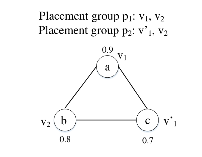
However, we cannot directly apply Eq. (3) to calculate its availability, since the availabilities of nodes which hold “shared” VMs will be counted more than once. To amend this, we use a new operator $\circ$¹¹ 1 As in [18, 19] for the partially link-disjoint paths connection availability.. Suppose there are $m$ different nodes $n_{1},n_{2},\ldots,n_{m}$ with availabilities $A_{1},A_{2},\ldots,A_{m}$. For a node $n_{x}$ with availability $A_{x}$, $\circ$ can be defined as follows:

Let $\coprod$ denote consecutive $\circ$ operations of the different sets, then the availability (represented by $A^{H}_{PD}$) of $H$ partially placement groups can now be represented as:

where $A_{p_{i}}$ denotes the availability of placement group $p_{i}$ and can be calculated from Eq. (2). Now, going back to the example of Fig. 1, when there are no communication requirements between the two requested VMs, the placement availability of $p_{1}$ and $p_{2}$ is equal to $1-(1-A_{a}\circ A_{b})\circ(1-A_{c}\circ A_{b})=A_{a}\circ A_{b}+A_{c}\circ A_{b}-A_{a}\circ\underline{A_{b}}\circ A_{c}\circ\underline{A_{b}}=A_{a}\cdot A_{b}+A_{c}\cdot A_{b}-A_{a}\cdot\underline{A_{b}}\cdot A_{c}=0.9\cdot 0.8+0.7\cdot 0.8-0.9\cdot 0.8\cdot 0.7=0.776$.

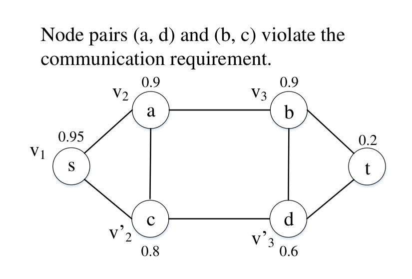
In order to emphasize the importance of communication requirements between the VMs, we consider the example of Fig. 2. For simplicity, it is assumed that each node can host at most one VM and its availability value is depicted in Fig. 2. Moreover, we impose that node pairs $(a,d)$ and $(b,c)$ have communication delays bigger than the requested delay, i.e., these two node pairs do not satisfy the VM communication requirement.

As is shown in Fig. 2, there are in total 4 possible placement groups: ($v_{1}$, $v_{2}$, $v_{3}$), ($v_{1}$, $v_{2}$, $v^{\prime}_{3}$), ($v_{1}$, $v^{\prime}_{2}$, $v_{3}$) and ($v_{1}$, $v^{\prime}_{2}$, $v^{\prime}_{3}$). However, neither ($v_{1}$, $v^{\prime}_{2}$, $v_{3}$) nor ($v_{1}$, $v_{2}$, $v^{\prime}_{3}$) can form a feasible placement group, because the communication delay is violated in either of these groups, and therefore, their availability cannot be taken into account.²² 2 As a side note, neglecting the communication requirement of VM pairs, the overall availability of the $4$ placement groups would have been: $1-(1-A_{s}\circ A_{a}\circ A_{b})\circ(1-A_{s}\circ A_{a}\circ A_{d})\circ(1-A_{s}\circ A_{c}\circ A_{b})\circ(1-A_{s}\circ A_{c}\circ A_{d})=0.89376$. As a result, we only take into account the two placement groups ($v_{1}$, $v_{2}$, $v_{3}$) and ($v_{1}$, $v^{\prime}_{2}$, $v^{\prime}_{3}$). According to Eq. (5), their overall availability is $1-(1-A_{s}\circ A_{a}\circ A_{b})\circ(1-A_{s}\circ A_{c}\circ A_{d})=A_{s}\circ A_{a}\circ A_{b}+A_{s}\circ A_{c}\circ A_{c}-\underline{A_{s}}\circ A_{a}\circ A_{b}\circ\underline{A_{s}}\circ A_{c}\circ A_{d}=A_{s}\cdot A_{a}\cdot A_{b}+A_{s}\cdot A_{c}\cdot A_{c}-\underline{A_{s}}\cdot A_{a}\cdot A_{b}\cdot A_{c}\cdot A_{d}=0.95\cdot 0.9\cdot 0.9+0.95\cdot 0.9\cdot 0.8-0.95\cdot 0.9\cdot 0.9\cdot 0.8=0.85614$.

We denote by $\mathcal{N}$ the set of $N$ server nodes and by $\mathcal{L}$ the set of $L$ links between them. The server nodes in $\mathcal{N}$ form a complete graph³³ 3 There is a possibility of all nodes to be connected, but the quality/goodness of these connections are determined by other factors (e.g., connection availability, communication delay). ($L=\frac{N(N-1)}{2}$). Each node $N_{j}\in\mathcal{N}$ has a storage upper bound of $s_{j}$. For each link $(m,n)\in\mathcal{L}$, a function $F(m,n,\eta,D)$ returns $1$ if $m$ and $n$ can have a connection availability of at least $\eta$ and communication delay of at most $D$, and $0$ otherwise. A request is denoted by $r(k,c,V,T,A,\delta)$, where $k$ indicates the requested number of VMs $V$ with demanding capacity $c_{v}$ ($v\in V$). $T$ and $A$ are $k\times k$ matrices, which specify the delay constraint and connection availability constraint between any two VMs, respectively, and $\delta$ is the requested VM placement availability.

Formally, the Reliable VM Placement (RVMP) problem is defined as follows:

In the RVMP problem, we assume that each VM can be placed at up to $H$ different nodes. Moreover, we only consider the server nodes and ignore some other nodes in the network (e.g., router nodes, switch nodes). In fact, the link between each node pair in the RVMP problem actually implies a (set of) path(s) which may traverse some other intermediate nodes. Finding reliable and delay-sensitive paths could be easier within a tree-like data center network, but this problem becomes harder when the node pairs are located in different data centers (a more general network). As we proved in [18, 19], the problem of finding $w\geq 2$ link-disjoint paths for which the connection availability is no less than a given value is already NP-hard and cannot be approximated to an arbitrary degree. In this sense, jointly considering the RVMP problem and reliable routing problem will make it even harder to solve. Therefore, we assume $F(m,n,\eta,D)$ is precalculated by using the algorithms proposed in Section VI, where we will address how to find reliable and delay-sensitive paths by taking link availability and link delay into account.

In this subsection, we propose an exact Integer Nonlinear Program (INLP) to solve the RVMP problem. We first solve the RVMP problem without SRNG failures and start by explaining the necessary notations and variables:

INLP notations:

$r(k,c,V,T,A,\delta)$: A VM placement request $r$ as specified in Section V-A.

$\mathcal{N},\mathcal{L}$: set of $N$ nodes and set of $L$ links, respectively.

$H$: The maximum number of times for one VM to be placed in the network.

$F(m,n,\eta,D)$ Returns $1$ if a connection exists between $m$ and $n$ such that connection availability is at least $\eta$ and communication delay value is at most $D$, and $0$ otherwise.

$\lambda_{i}^{n}$: The non-occurring probability of the $i$-th SRNG if node $n$ belongs to it, and $1$ otherwise.

INLP variable:

$P_{vn}^{h}$: a binary variable and it is equal to $1$ if VM $v$ is placed on node $n$ by placement group $h$, and $0$ otherwise, where $v\in V$, $n\in\mathcal{N}$ and $1\leq h\leq H$.

Objective:

Placement constraint:

Storage constraint:

Delay and connection availability constraint:

VM placement availability constraint:

Eq. (7) minimizes the number of total used nodes. For instance, we first calculate the maximum value of $P^{h}_{vn}$ for node $n\in\mathcal{N}$, and as long as $P^{h}_{vn}=1$ for some $1\leq h\leq H$ and $v\in V$, it means that node $n$ is in use to host VM(s). After that, we take the sum of $\max_{1\leq h\leq H,v\in V}P_{vn}^{h}$ for all the nodes in $\mathcal{N}$ and try to minimize this value. Eq. (8) ensures that each one of $k$ requested VMs must be placed in the network. Eq. (9) ensures that each node does not exceed its storage limit when VMs are placed on it. Eq. (10) makes sure that the specified delay constraint and connection availability of any two VMs under the same placement group are not violated. Eq. (11) ensures that the VM placement availability constraint is obeyed, according to Eq. (5). We note that Eq. (11) can simultaneously calculate the availability of the fully protected placement, partially protected placement, and single placement. For instance, when $H=2$, Eq. (11) becomes:

When $P_{vn}^{1}=P_{vn}^{2}$ for all $n\in\mathcal{N}$, Eq. (12) becomes

which is the VM placement availability constraint for the single placement.

To solve the RVMP problem with SRNG failures, we need to rewrite Eq. (11) in Eq. (13) and keep the objective and all other constraints the same (Eq. (7)-Eq. (10)).

Although inefficient in practice when the problem size is large, the INLP is useful for comparison purposes and demonstrates how accurate the heuristics are. This is shown in Figures 3 and 4 (for smaller size problems).

Our proposed heuristic to solve the RVMP problem, called the Delay-Sensitive and Reliable (DSR) placement algorithm, is shown in Algorithm 1. Instead of placing VMs on nodes, the logic of DSR is to assign nodes to VMs until all the VMs are hosted by the nodes without violating VM delay and connection availability constraints. Since we want to use the least number of nodes to host VMs to satisfy the availability requirement, we gradually increase the amount of finding placement groups. In what follows, we explain each step of the heuristic algorithm, where the SRNG failures are first not considered.

In Step $1$ of Algorithm 1, we first initialize a binary variable $VP[h][v][n]$ representing whether VM $v\in V$ is hosted by node $n\in\mathcal{N}$ under the group $h$. After that, for placement group $h$, we call Algorithm 2 to place VMs on nodes in Step $3$. The purpose of Step $4$ is to avoid different groups to have the same placement result. But this will only happen when a single node’s free capacity is far greater than the VM demanding capacity. That is, all the VMs can be placed on the same node and its remaining free capacity is still large enough so that another set of $k$ VMs can be placed on it. In Step $5$, we calculate the availability of $VP[1]$, …, $VP[h]$. If availability value of these $h$ placement groups is no less than $\delta$, we call Algorithm 3 trying to return a partially VM placement solution in order to further reduce the number of used nodes. In Algorithm 3, for each node $n\in\mathcal{N}_{y}$, where $\mathcal{N}_{y}$ stores the nodes in the increasing order by their availabilities, we first clear all the VMs resident on $n$. For each placement group $p$, we try to use its other used nodes to host the VMs that are originally placed by it on $n$. For simplicity, we apply a greedy approach: for each one (say $n_{u}$) of used nodes by placement group $h$, we let $n_{u}$ host the VMs which are originally placed on $n$ by $p$ as many as possible. After that, we calculate whether the whole availability still satisfies $\delta$. If so, we assign this partially placement solution to $VP$. Next, we will explain the details of Algorithm 2, which is to find a single placement.

In Step $1$ of Algorithm 2 we start with each $v_{m}\in V$, and assign it to $v_{x}$ in Step $2$. We use a queue $Q$ to store the VMs already placed, and initially it is set to empty. Besides, we also define variable $P^{m}[v][n]$ to indicate whether VM $v\in V$ is hosted by node $n\in\mathcal{N}$ corresponding to the placement group starting with VM $v_{m}$. As long as $Q$’s count is less than $k$, Step $4$-Step $9$ are going to assign nodes to host unassigned VMs. Step $5$ tries to find a node $n_{a}$ with maximum availability whose capacity should be at least $c(v_{x})$. Moreover, if $v_{x}$ is placed on $n_{a}$, it should not violate the delay and connection availability constraints with already hosted VMs. If it succeeds, in Step $7$, the capacity of $n_{a}$ is reduced by $c_{v_{x}}$, the availability of $n_{a}$ is changed to $1$, and $v_{x}$ is added to $Q$. The reason to change a node’s availability is that if some nodes have been used to host the existing VM(s), then the availability for these nodes to host other (unassigned) VMs is $1$. So we need to change its “availability” after each iteration of covering VM(s). If such a node cannot be found in Step $5$, this indicates that not all the VMs are covered and we consider this placement group should “jointly” place uncovered VMs with one of $H-1$ placement groups found in Algorithm 1. The algorithm then breaks in Step $9$. Following that, Step $10$-Step $14$ search for an unsigned VM, which has the smallest value of $\frac{T(v_{i},v_{j})\cdot\alpha}{A(v_{i},v_{j})}$ to the VMs already placed, where $\alpha$ is a user given value. By doing this, we want to find an unsigned VM that has “smaller” path delay and “greater” connection availability constraints with already placed VMs, and assigns it to $v_{x}$. The motivation here is that we always first place the VM which has a more critical requirement in terms of path delay and connection availability. When $Q$’s count is equal to $k$, it indicates that all the VMs have been hosted, which means we get a “complete” placement group. Finally, in Step $15$, the algorithm returns a placement group with the biggest availability from $k$ already determined single placements.

To solve the RVMP problem with SRNG failures, Alg. 1-3 remain the same except:

• •

  In Step $4$ of Algorithm 2 and Step $1$ of Algorithm 3, we sort the nodes in $\mathcal{G}^{m}$ by the product of their availabilities and non-occurring probabilities of all their belonging SRNG events in a decreasing order and an increasing order, respectively.

• •

  In Step $5$ of Algorithm 2, we will find one node $n_{a}$ with maximum node availability multiplied by the non-occurring probabilities of SRNG events set $R_{n_{a}}\backslash R_{x}$, where $R_{x}$ denotes the set of SRNG events that $n_{a}$ belongs to but has already been considered/counted by the other nodes from Step $4$ to Step $14$. The reason is that one unique SRNG event can only occur once, so we cannot calculate its value under the same placement group more than once.

The time complexity of Algorithm 2 can be calculated like this: There are $k$ VMs in total in Step $1$, and Step $3$ has also $k$ iterations. Sorting algorithm for instance like insertion sort in Step $4$ takes $O(N\log(N))$ time, and Step $5$ has a complexity of $O(N)$. Step $9$-Step $13$ consume at most $O(k^{2})$ time. Therefore, the whole complexity of Algorithm 2 is $O(k^{2}(N\log(N)+k^{2}))$. In Algorithm 3, Step $1$ consumes $O(N\log(N))$ time via insertion sort and Steps $2$-$8$ consume $O(N^{2}H)$ time, leading to a whole complexity of $O(N(\log N+NH))$. Consequently, the whole time complexity of Algorithm 1 is $O(k^{2}H(N\log(N)+k^{2}))$, since it calls at most $H$ times of Algorithm 2.

The simulations are run on a desktop PC with $2.7$ GHz and $8$ GB memory. We use an Intel(R)Core(TM)i5-4310M CPU 2.70GHz x64-based processor in our simulations. We use IBM ILOG CPLEX $12.6$ to implement the proposed INLP. All the heuristics are implemented by C# and compiled on Visual Studio 2015 (using .NET Framework 4.5).

We set $\alpha=1$ for our heuristic DSR. We compare our exact INLP and heuristic DSR with two heuristics, namely (1) Greedy Placement (GP) and (2) Random Placement (RP). These 2 algorithms follow the similar routine with Algorithm 1, except: (1) in Step $6$, they directly return the placement result if its availability is satisfied, instead of checking partially placement solution, and (2) they call different heuristics in Step $3$ (different from Algorithm 2), which we specify as follows:

• •

  GP (or RP): It first selects a node with greatest availability (or randomly selects a node) and places as many VMs as possible on it under its storage limit. It then selects the second largest availability node (or randomly selects the second node) and places as many of the remaining VMs as possible, which should also satisfy the delay and connection availability constraints with the VMs already placed. This procedure continues until all the VMs are placed or all the nodes have been iterated.

In the following, we first test the algorithms for the RVMP problem without SRNG failures for both $16$-node and $100$-node networks, and then evaluate them for the RVMP problem with SRNG failures for a $100$-node network.

Analogous to the node failure scenarios, we also address two kinds of link failure scenarios. For simplicity, suppose there are two (fully) link-disjoint paths $\psi_{1}$ and $psi_{2}$, and the availability of link $l$ is denoted as $A_{l}=1-f_{l}$, where $0<A_{l}\leq 1$ and $f_{l}$ is the failure probability of link $l$. Then their total availability $A^{2}_{FD}$ can be computed based on the following scenarios:

• •

  Single-link failure: Analogous to the single node failure, here a path $\psi$’s availability (denoted by $A_{\psi}$) is equal to its lowest traversed link availability (highest failure probability). Using two disjoint paths will therefore lead to a total connection availability of $1$. In Appendix B, we will address the ABDCR problem under the single-link failure scenario.

• •

  Multiple link failures: This is a more general scenario where at one certain point in time, several links in the network may fail simultaneously. Hence, for a path $\psi$, its availability $A_{\psi}$ should take into account all its links’ availabilities, i.e., $A_{\psi}=\prod_{l\in\psi}A_{l}$. Consequently, $A^{2}_{FD}=1-(1-A_{\psi 1})(1-A_{\psi 2})$, which indicates the probability that at least one of the two disjoint paths is available. In this paper, we assume multiple link failures may occur at any particular time point.

Similar to the node availability, we assume that the link availability is equal to the product of availabilities of all its components (e.g., amplifiers). If a path $p$ contains the links $l_{1}$, $l_{2}$, $l_{3}$,…, $l_{m}$, and their corresponding (independent) availabilities are denoted by $A_{l_{1}}$, $A_{l_{2}}$, $A_{l_{3}}$,…, $A_{l_{m}}$, then the availability of this (unprotected) path (represented by $A_{\psi}$) is equal to $A_{\psi}=A_{l_{1}}\cdot A_{l_{2}}\cdot A_{l_{3}}\cdot\cdots\cdot A_{l_{m}}$. If we take the $-\log$ of the link availabilities, finding a path with the highest availability is equivalent to the shortest path problem [27].

When, for a single connection (i.e., a single path), there are $w\geq 2$ paths $\psi_{1}$, $\psi_{2}$,…, $\psi_{w}$ with availabilities represented by $A_{\psi_{1}}$, $A_{\psi_{2}}$,…, $A_{\psi_{w}}$, the connection availability indicates the probability that at least one path is operational. We consider two cases, namely: (1) fully link-disjoint paths: these $w$ paths have no links in common, and (2) partially link-disjoint paths: at least two of these $w$ paths traverse a common link. In case (1), the availability (represented by $A^{w}_{FL}$) can be calculated as follows:

If we use Eq. (14) to calculate the availability for the partially link-disjoint case, the probability that the overlapping links operate (or the availability of the overlapping links) will be counted more than once. To solve this, we can analogously apply the operators $\circ$ and $\coprod$ introduced in Section III. Assuming there are $w$ partially link-disjoint paths $\psi_{1}$, $\psi_{2}$,…, $\psi_{w}$, the availability (represented by $A^{w}_{PL}$) of $w$ partially link-disjoint paths can be calculated as:

Let us use an example to explain how to calculate the connection availability for fully and partially link-disjoint paths, where $w$ is set to $2$ for simplicity. In Fig. 8 where the link availability is labeled on each link, paths $s-a-t$ and $s-b-t$ are fully link disjoint. According to Eq. (14), their availability is equal to:

On the other hand, paths $s-a-t$ and $s-a-b-t$ are two partially link-disjoint paths. According to Eq. (15), the connection availability can be calculated as follows:

References

- [1] S. Yang, P. Wieder, and R. Yahyapour, “Reliable virtual machine placement in distributed clouds,” in Proc. of 8th IEEE/IFIP International Workshop on Reliable Networks Design and Modeling (RNDM), 2016, pp. 1-7.
- [2] P. Mell and T. Grance, “The NIST definition of cloud computing,” Communications of the ACM, vol. 53, no. 6, p. 50, 2010.
- [3] B. Jennings and R. Stadler, “Resource management in clouds:Survey and research challenges,” Journal of Network and Systems Management, pp.1-53, 2014.
- [4] Z. Á. Mann, “Allocation of virtual machines in cloud data centers—-a survey of problem models and optimization algorithms,” ACM Computing Surveys (), vol. 48, no. 1, p. 11, 2015.
- [5] M. Alicherry and T. Lakshman, “Network aware resource allocation in distributed clouds,” in Proc. of IEEE INFOCOM, 2012, pp. 963-971.
- [6] O. Biran, A. Corradi, M. Fanelli, L. Foschini, A. Nus, D. Raz, and E. Silvera, “A stable network-aware vm placement for cloud systems,” in Proc. of 12th IEEE/ACM International Symposium on Cluster, Cloud and Grid Computing (CCGRID), 2012, pp. 498-506.
- [7] J. W. Jiang, T. Lan, S. Ha, M. Chen, and M. Chiang, “joint vm placement and routing for data center traffic engineering,” in Proc. of IEEE INFOCOM, 2012, pp. 2876-2880.
- [8] X. Meng, V. Pappas, and L. Zhang, “Improving the scalability of data center networks with traffic-aware virtual machine placement,” in Proc. of IEEE INFOCOM, 2010, pp. 1-9.
- [9] A. Israel and D. Raz, “Cost aware fault recovery in clouds,” in Proc. of IFIP/IEEE International Symposium on Integrated Network Management (IM), 2013, pp. 9-17.
- [10] E. Bin, O. Biran, O. Boni, E. Hadad, E. K. Kolodner, Y. Moatti, and D. H. Lorenz, “Guaranteeing high availability goals for virtual machine placement,” in Proc. of 31st IEEE International Conference on Distributed Computing Systems (ICDCS), 2011, pp. 700-709.
- [11] Y. Zhu, Y. Liang, Q. Zhang, X. Wang, P. Palacharla, and M. Sekiya, “Reliable resource allocation for optically interconnected distributed clouds,” in Proc. of IEEE International Conference on Communications (ICC), 2014, pp.3301-3306.
- [12] X. Li and C. Qian, “Traffic and failure aware VM placement for multi-tenant cloud computing,” in IEEE 23rd International Symposium on Quality of Service (IWQoS), 2015, pp. 41-50.
- [13] Z. Yang, L. Liu, C. Qiao, S. Das, R. Ramesh, and A. Y. Du, “Availability-aware energy-efficient virtual machine placement,” in IEEE International Conference on Communications (ICC), 2015, pp. 5853-5858.
- [14] L. Song, J. Zhang, and B. Mukherjee, “Dynamic provisioning with availability guarantee for differentiated services in survivable mesh networks,” IEEE Journal on Selected Areas in Communications, vol. 25, no. 3, pp. 35-43, 2007.
- [15] Q. She, X. Huang, and J. Jue, “How reliable can two-path protection be?” IEEE/ACM Transactions on Networking, vol. 18, no. 3, pp. 922-933, 2010.
- [16] H. Luo, L. Li and H. Yu, “Routing connections with differentiated reliability requirements in WDM mesh networks,” IEEE/ACM Transactions on Networking, vol. 17, no. 1, pp. 253-266, 2009.
- [17] H.-W. Lee, E. Modiano, and K. Lee, “Diverse routing in networks with probabilistic failures,” IEEE/ACM Transactions on Networking, vol. 18, no. 6, pp. 1895–1907, 2010.
- [18] S. Yang, S. Trajanovski, and F. Kuipers, “Availability-based path selection,” in Proc. of 6th IEEE International Workshop on Reliable Networks Design and Modeling (RNDM), 2014, pp. 39-46.
- [19] S. Yang, S. Trajanovski, and F. Kuipers, “Availability-based path selection and network vulnerability assessment,” Networks, vol. 66, no. 4, pp. 306-319, 2015.
- [20] J. I. McCool, Probability and Statistics With Reliability, Queuing and Computer Science Applications. Taylor & Francis, 2003.
- [21] K. V. Vishwanath and N. Nagappan, “Characterizing cloud computing hardware reliability,” in Proc. of the 1st ACM symposium on Cloud computing, 2010, pp. 193-204.
- [22] P. Gill, N. Jain, and N. Nagappan, “Understanding network failures in data centers: measurement, analysis, and implications,” in ACM SIGCOMM Computer Communications Review, vol. 41, no. 4, 2011, pp. 350-361.
- [23] P. Datta and A. K. Somani, “Graph transformation approaches for diverse routing in shared risk resource group (srrg) failures,” Computer Networks, vol. 52, no. 12, pp. 2381-2394, 2008.
- [24] C. Kachris, K. Bergman, and I. Tomkos, Optical interconnects for future data center networks. Springer Science & Business Media, 2012.
- [25] M. R. Garey and D. S. Johnson, Computers and Intractability: A Guide to the Theory of NP-Completeness. New York, NY, USA: W. H. Freeman & Co., 1979.
- [26] M. Alicherry and T. Lakshman, “Optimizing data access latencies in cloud systems by intelligent virtual machine placement,” in IEEE INFOCOM, 2013, pp. 647-655.
- [27] E. W. Dijkstra, “A note on two problems in connexion with graphs,” Numerische mathematik, vol. 1, no. 1, pp. 269-271, 1959.
- [28] P. Van Mieghem and F. A. Kuipers, “Concepts of exact quality of service algorithms,” IEEE/ACM Transactions on Networking, vol. 12, no. 5, pp. 851–864, 2004.
- [29] B. Mukherjee, Optical WDM Networks. Springer Science & Business Media, 2006.
- [30] P. Van Mieghem, “Paths in the simple random graph and the waxman graph,” Probability in the Engineering and Informational Sciences, vol. 15, no. 04, pp. 535-555, 2001.
- [31] T. H. Cormen, C. Stein, R. L. Rivest, and C. E. Leiserson, Introduction to Algorithms, 2nd ed. Cambridge, MA: MIT Press, 2001.
- [32] C.-L. Li, S. T. McCormick, and D. Simchi-Levi, “The complexity of finding two disjoint paths with min-max objective function,” Discrete Applied Mathematics, vol. 26, no. 1, pp. 105-115, 1990.