Algebraic Properties of Wyner Common Information Solution under Graphical Constraints
Abstract
The Constrained Minimum Determinant Factor Analysis (CMDFA) setting was motivated by Wyner’s common information problem where we seek a latent representation of a given Gaussian vector distribution with the minimum mutual information under certain generative constraints. In this paper, we explore the algebraic structures of the solution space of the CMDFA, when the underlying covariance matrix has an additional latent graphical constraint, namely, a latent star topology. In particular, sufficient and necessary conditions in terms of the relationships between edge weights of the star graph have been found. Under such conditions and constraints, we have shown that the CMDFA problem has either a rank one solution or a rank solution where is the dimension of the observable vector. Numerical results are provided to demonstrate the difference between the optimal mutual information and that derived under a naive star constraint.
Index Terms:
Factor Analysis, MTFA, CMTFA, CMDFAI INTRODUCTION
Factor Analysis (FA) is a commonly used tool in multivariate statistics to represent the correlation structure of a set of observables in terms of significantly smaller number of variables called “latent factors”. With the growing use in data mining, high dimensional data analytics, factor analysis has already become a prolific area of research [1][2]. Classical Factor Analysis models seek to decompose the correlation matrix of an -dimensional random vector , , as the sum of a diagonal matrix and a Gramian matrix .
The literature that approached Factor Analysis can be classified in three major categories. Firstly, algebraic approaches [3] and [4], where the principal aim was to give a characterization of the vanishing ideal of the set of symmetric matrices that decompose as the sum of a diagonal matrix and a low rank matrix, did not offer scalable algorithms for higher dimensional statistics. Secondly, Factor Analysis via heuristic local optimization techniques, often based on the expectation maximization algorithm, were computationally tractable but offered no provable performance guarantees. The third and final type are the convex optimization based methods such as Constrained Minimum Trace Factor Analysis (CMTFA) [5] [6] and CMDFA [7]. The motivation behind CMDFA comes from Wyner’s common information which characterizes the minimum amount of common randomness needed to approximate the joint density between a pair of random variables and to be , where is the mutual information between , and , indicates the conditional independence between and given , and the joint density function is sought to esnure such conditional independence as well as the given joint density of and . Since the Factor Analysis of the Gaussian random vector can be modelled as , where is a real matrix, is the vector of independent latent variables and is a Gaussian vector of zero mean and covariance matrix . Hence we have, where is the mutual information between and , are differential entropies of and and is the differential entropy of given . Hence characterizing the common information between and [8][9][10] would be which is an equivalent problem to hence equivalent to .
The scope of this paper is limited to analysing the solution space of CMDFA and recovering the underlying graphical structures. It is important to remark that our work is not concerned about the algorithm side of the optimization technique, rather our focus is to characterize and find insights about their solution space. Moharrer and Wei [7] derived CMDFA from a broader class of convex optimization problem and established a relationship between the outcome of these optimization techniques and common information problem [9]. We find the explicit conditions under which the CMDFA solution of recoves a star structure. Since star may not always be the optimum solution, we have also shown the existence and uniqueness of a rank CMDFA solution of which is the only other possible solution. We have shown analyticaly the optimality of the non-star solution over star under certain circumstances from common information point of view, and at the end presened some numerical data to support our claims.
II Definitions and Notations
Let be a real dimensional column vector and be an matrix. As in literature in general we denote the th element as and the th element of as . Here we define all the vector operations and notations in terms of and , that will carry their meaning on other vectors and matrices throughout this paper unless stated otherwise.
Let and denote the th row and th column vector of matrix respectively. Function is defined to be the smallest eigen value of matrix . stands for the null space of matrix .
Vectors and are the dimensional column vectors with each element equal to and respectively. When we write we mean that each element of the vector . is the Hadamard product of vector with itself. denotes the norm of vector .
Now we define two terms i.e. dominance and non-dominance of a vector which will repeatedly appear throughout the paper. When we talk about the dominance or non-dominance of any vector we assume that the elements of the vector are sorted in a way such that . We call vector dominant and the dominant element if for the above sorted vector holds. Otherwise is non-dominant.
III Formulation of the Problem
First of all we define the real column vector as where , and
| (1) |
Let us consider a star structured population covariance matrix having all the diagonal comptonents as given by equation (2).
| (2) |
The above covariance matrix could be produced by the graphical model given by equation (3).
| (3) | ||||
| (4) |
where
- •
are conditionally independent Gaussian random variables given , forming the jointly Gaussian random vector where .
- •
are independent Gausian random varables with forming the Gaussian random vector .
The above graphical model assumes the conditional independence among the observables given the latent variable given by (5) giving rise to a star topology.
| (5) |
CMDFA aims to minimize the mutual information between the observable Gaussian random vector and the latent ones . It is thus to seek joint distribution between the latent and observable ones such that the differential entropy is maximized. Under the joint Gaussian distribution, it is the same as seeking factorization of such that the determinant of the matrix is minimized as in equation (6) under the constraint that both and are Gramian matrices.
| (6) |
being produced by the model in (3) would equivalently mean (6) having a rank solution i.e. being given by equation (7).
| (7) |
But CMDFA solution of may not always be rank , indicating star may not always be the optimum solution from common information point of view. It remains to be seen if CMDFA solution to recovers the graphical model given by (3). Also to be investigated is the exact solution to CMDFA if it fails to recover the underlying star topology. In the rest of the paper, we will present both sufficient and necessary conditions under which the rank of the optimal and the values of ’s entries are determined.
IV Solutions to CMDFA
In this section we present the detailed analysis of the CMDFA solution space of . We defne the real column vector as where .
As we can see, each elements in is equal to the square root of the signal to noise ratio () of the corresponding element of vector . The following order of the elements of is a necessary consequence of our assumption in (1),
| (8) |
As we metioned before, we are interested to find out if CMDFA low rank decomposition of produces a rank matrix. Next we analyse the solution space of CMDFA and find explicit conditions for both when the solution is rank and when it is not. To start the proceedings we state Theorem 1 given in [7] that gives the necessary and sufficient condition for to be the CMDFA solution of the decomposition given in (6).
Theorem 1.
The matrix is the CMDFA solution of if and only if , and there exists matrix such that and .
In the first of the two subsections of this section, we find the conditions under which CMDFA solution of recovers the model given by (3) or equivalently speaking, find condtions under which CMDFA solution of is the rank matrix given by (7). In the other subsection, we show the detailed analysis on the existance and uniqueness of the CMDFA solution of , when the solution is not a rank matrix.
IV-A CMDFA Non-dominant Case
Here we analyse the conditions under which the CMDFA solution of recovers a star structure. Lemma 1 sets the groundwork for the Theorem to follow. The Lemma also has a geometric interpretaion that enriches our overall understanding of the CMDFA non-dominant case.
Lemma 1.
There exists matrix such that and if and only if vector is non-dominant i.e.,
| (9) |
Proof of Lemma 1:.
Let be the th row vector of the matrix and denote the zero column vector. We need,
| (10) |
Equation (10) has a beautiful geometric interpretation. The length of each vector can be written as,
| (11) |

Hence, each vector is a point on the surface of an dimensional sphere of radius . Equation (10) dictates that, for the matrix to be in the null space of the biggest of those spheres can not have a radius greater than the sum of the other radiuses. This leads us to the condition of non-dominance. Using (10),
∎
For further clarification, we refer to the co-centric spheres (assuming ) in Figure 1. Let , , . If , it is impossible to find any vector on the outer most sphere that can be expressed as the vector sum of vectors and . On the other hand if proper selection of angles and can always ensure be a vector sum of and or equivalently ensure the orthogonality given by .
Having proved Lemma 1 we are now well equipped to state and prove the statement of Theorem 2 that has the main result of this subsection.
Theorem 2.
CMDFA solution of is if and only if is non-dominant.
The theorem states that the CMDFA solution to a star connected network is a star itself, if and only if there is no dominant element in the vector .
Proof of Theorem 2:.
Now we refer back to the necessary and sufficient condition for CMDFA solution at the begining of this section given by Theorem 1. Since, in rank , its minimum eigenvalue is . To complete the proof of Theorem 2, we only need to show the existance of matrix such that the column vectors of are in the null space of and the -norm square of the th row of is .
Lemma 1 has already shown that, for the existence of such non-dominance given by equation (9) is a necessary condition. Next we show, by constructing such a matrix under the assumption of non-dominance of , that non-dominace is also a sufficient condition . And that should complete the proof of Theorem 2.
It is straightforward to find the following basis vectors for the null space of ,
| (12) |
We define matrix so that its columns span the null space of ,
| (13) |
where and .
The columns of span the null space of . To construct our desired matrix , under the assumption of non-dominance of , it will suffice for us to find a diagonal matrix such that the following holds.
| (14) |
where the -norm square of the th row of is . Using (14),
| (15) |
We require the diagonal matrix to have only non-negative entries. Based on the conditions imposed on the matrix , we have the following equations,
| (16) |
| (17) |
Solving, (16) with the help of (17) we get,
| (18) |
It is straightforward to see that, to ensure all the are non-negative, we need . We select such that,
| (19) |
Under such selection of , becomes,
| (20) |
Now, using the non-dominance assumption given in (9), we have
| (21) | ||||
| (22) |
Which means non-dominance of vector is a sufficient condition to construct the kind of matrix we are looking for. That completes the proof of Theorem 2. ∎
Boundary Case
It is obvious that, there might be numerous ways to construct the matrix that satisfisfy the requirements set by Theorem 1. Because of the special way we constructed the matrix the rank of under the non-dominant case is except for a very special boundary case. Under the boundary case i.e. when the inequality (9) holds for equality, when the rank of is always irrespective of the way we construct . For any given , it is straightforward to see from equation (21) that, for we have . Plugging in equation (17) gives us . Equations (14) and (15) suggest that, such a matrix will produce a rank matrix . This very special case is explained by the next Lemma.
Lemma 2.
When the non-dominance condition given in (9) holds for equality, any matrix such that and has to be a rank matrix.
Proof of Lemma 2:.
Using the orthogonality between and its null space matrix ,
| (23) |
Equation (23) implies the following two things:
| (24) | ||||
| (25) |
Using the triangular inequality,
| (26) |
If all the are not in the same direction, the the above inequality becomes
| (27) |
Hence, under the boundary condition i.e. , we have
Which violets (24). That means to ensure , all of have to be in the same direction. This along the second implication of orthogonality given by equation (25), makes matrix a rank matrix. ∎
IV-B Dominant Case
Having proved that the non-dominance of vector is a sufficient and necessary condition for CMDFA solution of to recover a star structure, we are left with only the dominance case now i.e.
| (28) |
Under the above dominant condition we want to show the existence of a rank solution of . Any solution we find will be unique, because CMDFA is a special type of the broader class of convex optimization problem defined in [11]. We still have to satisfy the same sufficient and necessary condtion for the CMDFA solution, that we presented at the begining of this section. Like the non-dominant case, for the matrix to be the CMDFA solution of under the dominant case, the minimum eigen value of has to be and the -norm square of the th row of the null space matrix has to be . The only difference with the non-dominant case is that, since our conjecture for the dominant case is an rank solution, the null space matrix will always be rank i.e. a column vector. Mathematically speaking, we need to show the existance of such that the following orthogonality condition holds.
| (29) |
where . Once we have such the th element of the CMDFA solution vector under the dominant case will be . The above orthogonality relationship gives us the following equations.
| (30) |
Let denote the th equation given by (30). Using the linear combination gives us the following equations.
| (31) |
where
| (32) |
Equation (51) implies that for some ratio we can write the following,
| (33) |
Now plugging the expressions from (32) and (33) in any of the equations given by (30) we get,
| (34) |
It will suffice for us to prove the existence of such that (34) holds. From the definition of given in (32) we see that, to find each we need to solve the following second order polynomial.
| (35) |
If we solve equation (35) for each we will get a left root and a right root. Our initial conjecture is that the left root for and right roots for that we get solving (35) will give us that satisfy (34). If we can prove that our conjecture is true, then that should be the only possible solution to (34) because of the uniqueness of solution to such convex optimization problems proved in [11]. Plugging in the left root for , right roots for in (34) gives us the following equation.
| (36) |
We define
| (37) |
Under these newly defined s (36) becomes,
| (38) |
And using the definition of given in (37), we get the following cylinders of hyperbolas.
| (39) |
Equations given by (39) imply that for each value of we get a point in the dimensional space where each is a function of . For the range of values of all such points together produce an dimensional space curve. If we project this space curve on any of the two dimensional planes we get a hyperbola.
Another important thing to note is that, each equation given by (39) is a cylinder of hyperbolas originated from plane and projected onto dimensional space. Each point in the space curve represents an intersection points of all cylinders of hyperbolas originated from planes.
At this point our revised goal is to show the existence of a point in the space curve that satisfies equation (38) under the dominance condition given by (28). Becasue of the way we defined s the solution must satisfy the condition . Theorem 3 states the main result of this subsection.
Theorem 3.
Proving the above Theorem would mean that, there exists such that (34) holds, which in turn would mean the existance of an rank CMDFA solution under the dominance of vector . And as we mentioned already, the uniqueness of such solution is guaranteed.
Proof of Theorem 3:.
Let us define the function of as the inner product between the vectors and where each is a function of . Which means,
| (40) |
So, our revised goal becomes to find the existence of such for which the function of becomes . And to achieve that goal some functional analysis of that we present next are of paramount importance.


Equation (39) dictates that each is a concave function of . Which makes given by (40) a convex function of as the sum of convex functions of . Using (39) and (40) we get,
| (41) |
Using (37) we get,
| (42) |
| (43) |
Hence,
| (44) |
which is a negative value. We define such that,
| (45) |
Figures 2 and 3 illustrate our findings from the above functional analysis. As each is an increasing function of the ratios are decreasing functions of . Hence equation (43) suggests that is an increasing function of . Given that knowledge, equations (44) and (45) considered together imply as seen in Figures 2 and 3. One important to remark is that we see the function gets saturated gradually and is upperbounded by a value. This is because the ratio is the slope of hyperbola in plane which is upper bounded by which is the slope of the asyptote in the respective plane. Plugging these individual upperbounds in (42) we get the dotted upper bound in Figure 3.
From Theorem 3 and its proof we know that the solution produces a corresponding dimensional point in the space curve which is the intersection point among hyperbolic cylinders and the plane given by (39) and (38) respectively. If we reflect on the bigger picture, plugged in (37) will produce a value of which in turn plugged in (35) will give us a set of that satisfies (29).
IV-B1 Bounds of the Solution
Here we find a lowerbound and an upperbound to .
Upperbound to : It is easy to derive that the th hyperbolic cylinder given by (39) has the following corresponding equation of the cylinder asymptotes (the ones passing through the origin and the first quadrant of the respective plane).
| (46) |
Solving (46) and (38) together we get a value of which we denote as given by (47),
| (47) |
Substituting in (46) by gives us a vector in the dimensional space, which is the intersection of the cylinders of asymptotes in (46) and the plane in (38).
Lemma 3.
The prooof of Lemma 3 is given in Appendix A. According the statement of this Lemma . Which immediately suggests that given by (47) is an upperbound on .
Lowerbound to : We see in Figure 2 that the average slope of the curve is captured by the slope of the line . We assume that the dashed line in Figure 2 has slope i.e. the upperbound of given in Figure 3. Figure 3 suggests that, the slope at each point of the curve is strictly less than the slope of in Figure 2, hence the slope of must be less than the slope of . Now considering triangles and in Figure 2 we have,
| (48) |
Which suggests a lowerbound of the actual . Next we find the expression for using the geometry in Figure 2.
| (49) |
V Numerical Data
We motivated CMDFA in terms common information which is a function of the minimum mutual information between the observables and the latent factors. It is a common practice to assume the star topology i.e the assumption that all the observables are mutually independent given a latent factor. Though star offers a sparce structure and smooth analysis, it may not be always the optimum solution. Next we show that assumption of star under CMDFA dominant case does not produce optimum outcome from common information point of view. We show that under the dominant case CMDFA solution provides lower mutual information between the observables and the latent variables that the star solution. Which in turn means lower common randomness required to produce the joint distribution between the observables and the latent variables and hence lower Wyner common information. In summary, we are about to demonstrate the additional cost in using more information bits to synthesize -dimensional Gaussian vector under a star topology, when we do not use the solution of CMDFA, under the dominant case.
As mentioned before, each of and will produce a corresponding from equaion (37) and a set or equivalently produce a matrix that decomposes (6). Let and produce and from equaion (37), the corresponding sets and from (35), corresponding matrices and that decompose (6), and , be the corresponding mutual information between observed variables and the latent variables respectively. Also let be the solution to (6) when the CMDFA solution is a star and be the corresponding mutual information between the observed variables and the latent factor . Next Theorem analytically shows that each of , produces better results than considered from common information point of view. We present the comparative results with respect to the varying magnitude of the dominance of . Referring to equation (28), we vary the dominance of vector by changing the value of the first element while keeping other elements unchanged.
Theorem 4.
All of , and are increasing functions of

The proof of Theorem 4 is given in Appendix B. Figure 4 presents , and as functions of for a particular case of , where is the mutual information between the observed variables and the latent ones corresponding to the numerically found solution . As we mentioned in the introduction that the primary motivation for this part of the work comes from common information, and the fact that in general people tend to assume a star topology to find common information, any value of mutual information less than works to our advantage. is an increasing function of indicates that the lower bound of the advantage of CMDFA solution over star increases as vector becomes more and more dominant. We numerically calculated and the curve in Figure 4 gives the actual advantage that CMDFA soution has over star under the dominance of whereas gives an upperbound to the actual advantage of CMDFA over a star topology. The gap between and is gradually increasing indicating is increasing with which justifies the statement of Theorem 4.
VI Conclusion
In this paper we analyzed the solution spaces of convex optimization algorithm CMDFA. We found conditions under which the solution is a star (rank ) and proved the existence of a rank solution when the solution is not a star. Through analytical analysis followed by numerical data we showed that star is not always the optimum solution. We particularly demonstrated the additional cost in using more information bits to synthesize -dim Gaussian vector under a star topology, when we do not use the solution of CMDFA, under the dominant case.
Appendix A •
Proof of Lemma 3:.
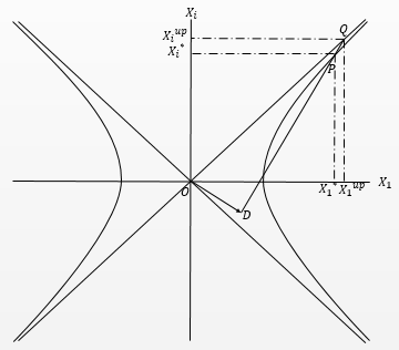
Let be the CMDFA solution vector i.e. the intersection point of (39) and (38). We refer to Figure 5, the CMDFA dominant case solution vector has been projected on the plane which is shifted in the direction of by . The procection of the dimensional plane given by (38) on this plane is given by the line which is at a perpendicular distance (because ) from the origin. Here is the projection of the vector on plane, whose length we can calculate from equation (38) as,
| (50) |
Geometrically, we can see in Figure 5 that the line which is the projection of the plane cuts the hyperbola at point and the corresponding asymptote at point in the first quadrant of the plane. It is obvious to notice that, because of the higher elevation and sharper slope of the asymptote compared to the hyperbola, point has higher coordinate values than point which is the projection of the CMDFA solution vector on plane i.e. and . The above conclusion holds true for any projection of on any plane. For example, the projection on plane will give us and . Combining the outcome of all such projection for we can conclude that . Which algebraically means, the intersection point among the hyperbolic cylinders in (39) and the plane in (38) is upper bounded by the intersection point among the asymptotes of the respective hyperbolic cylinders given by (46) and the plane in (38). ∎
Appendix B •
Proof of Theorem 4:
Before we go into the business part of the proof we do some general preparatory groundwork. Using Equation (35) and the fact that we used the right root of we get,
| (51) |
Similarly, since we are using the right roots for we get,
Equations (49) and (47) suggest that both and are decreasing functions of . And in turn equation (37) suggests that are increasing functions of . Since are constants, the only thing changing in (B) is . But can not increase beyond because that would mean equation (34) does not have a solution. Hence, in order to increase as we keep on increasing the value of and make it closer and closer to , the value of also gets closer to . Thus with the increament of the parameters given by (B) asymptotically converge to constants which we get plugging in i.e. for
| (53) |
Now that we have the groundwork done, we can proceed to prove the actual statement of the theorem.
| (54) |
is asymptotically a constant. Equation (37) suggests is an increasing function of because is a decreasing function of . Hence from (51),
| (55) |
Which is an increasing function of . Hence from (54) we see that is an increasing function of . Similarly,
| (56) |
Like the previous case we can argue that, is asymptotically a constant. Equation (37) suggests is an increasing function of because is a decreasing function of . Hence and consequently is an increasing function of .
Using equations (54) and (56),
| (57) |
where is a constant. Since and are increasing functions of and respectively, to show is an increasing function of we need to show is an increasing function of . Equations (49) and (47) suggest that is an increasing function of , and in turn (37) suggests is an increasing function of . That completes the final part of the proof. ∎
References
- [1] Y. Chen, X. Li, and S. Zhang, “Structured latent factor analysis for large-scale data: Identifiability, estimability, and their implications,” arXiv preprint arXiv:1712.08966, 2017.
- [2] D. Bertsimas, M. S. Copenhaver, and R. Mazumder, “Certifiably optimal low rank factor analysis,” Journal of Machine Learning Research, vol. 18, no. 29, pp. 1–53, 2017.
- [3] A. A. Albert, “The matrices of factor analysis,” Proceedings of the National Academy of Sciences, vol. 30, no. 4, pp. 90–95, 1944.
- [4] M. Drton, B. Sturmfels, and S. Sullivant, “Algebraic factor analysis: tetrads, pentads and beyond,” Probability Theory and Related Fields, vol. 138, no. 3-4, pp. 463–493, 2007.
- [5] P. Bentler and J. A. Woodward, “Inequalities among lower bounds to reliability: With applications to test construction and factor analysis,” Psychometrika, vol. 45, no. 2, pp. 249–267, 1980.
- [6] M. M. Hasan, S. Wei, and A. Moharrer, “Latent factor analysis of Gaussian distributions under graphical constraints,” 2018. [Online]. Available: http://arxiv.org/abs/1801.03481
- [7] A. Moharrer and S. Wei, “Agebraic properties of solutions to common information of gaussian graphical models,” in Communication, Control, and Computing (Allerton), 2017 55th Annual Allerton Conference on. IEEE, 2017.
- [8] G. Xu, W. Liu, and B. Chen, “A lossy source coding interpretation of wyner’s common information,” IEEE Transactions on Information Theory, vol. 62, no. 2, pp. 754–768, 2016.
- [9] A. Wyner, “The common information of two dependent random variables,” IEEE Transactions on Information Theory, vol. 21, no. 2, pp. 163–179, 1975.
- [10] S. Satpathy and P. Cuff, “Gaussian secure source coding and wyner’s common information,” in Information Theory (ISIT), 2015 IEEE International Symposium on. IEEE, 2015, pp. 116–120.
- [11] G. Della Riccia and A. Shapiro, “Minimum rank and minimum trace of covariance matrices,” Psychometrika, vol. 47, no. 4, pp. 443–448, 1982.