Another common approach for pdf estimation, and the one pursued in the current paper, is a two-step estimation procedure discussed in Leonard (1978); Lenk (1988); Lenk (1991); Tokdar et al. (2010); Tokdar (2007), etc. In the first step, one estimates an initial pdf, say $f_{p}$, from the data, perhaps restricting to a parametric family. Then, in the second step, one improves upon this estimate by forming a function $w>0$, that depends on the initial estimate $f_{p}$, and forming a final estimate using $w(x)f_{p}(x)/\int_{y}w(y)f_{p}(y)yd$. Thus, the second step involves estimation of an optimal $w$ in order to estimate the overall pdf. In a Bayesian context, the function $w$ is often assigned a Gaussian process prior. While this approach is quite comprehensive, the calculation of the normalization constant makes the computation very cumbersome. The two-step procedures can also be adapted for estimating conditional density functions: first estimate the conditional mean function and then estimate the conditional density of the residuals, as is done in Hansen (2004). Over the recent years, Bayesian methods for estimating pdfs based on mixture models and latent variables have received a lot of attention, primarily due to their excellent practical performances and an increasingly rich set of algorithmic tools for sampling posterior using Markov Chain Monte Carlo (MCMC) methods. References include Escobar and West (1995); Müller et al. (1996); MacEachern and Müller (1998); Kalli et al. (2011); Jain and Neal (2012); Kundu and Dunson (2014); Bhattacharya et al. (2010) among others. However, these results also come at a very high computational cost typically associated with the MCMC algorithms. Applications of flexible Bayesian models for conditional densities are discussed in MacEachern (1999); De Iorio et al. (2004); Griffin and Steel (2006); Dunson et al. (2007); Chung and Dunson (2009); Norets and Pelenis (2012), among others. Although the literature suggests that such methods based on mixture models have several attractive properties, they lack interpretability and the MCMC solutions for model fitting are overly complicated and expensive.

In this article, we pursue a geometric, two-step approach that is applicable to both conditional and unconditional density estimation. The main motivation here is develop an efficient estimation procedure while retaining good estimation performance. The main difference from the previously described two-step procedure is that the transformation of $f_{p}$ (in the second step) is now based on the action of a diffeomorphism group, as follows. Let $f_{p}$ be a strictly positive univariate density on the interval $[0,1]$; $f_{p}$ serves as an initial estimate of the pdf. Let $\Gamma$ be the set of all positive diffeomorphisms from $[0,1]$ to itself, i.e. $\Gamma=\{\gamma|\gamma\text{ is differentiable},{\gamma}^{-1}\text{ is differentiable, }\dot{\gamma}>0,\gamma(0)=0,\gamma(1)=1\}$. The elements of $\Gamma$ play the role of warping functions, or transformations of $f_{p}$. Given a $\gamma\in\Gamma$, the transformation of $f_{p}$ is defined by: $(f_{p},\gamma)=(f_{p}\circ\gamma)\dot{\gamma}$. Henceforth, this transformation is referred to as warping of $f_{p}$, and the resulting pdf $f$ as a warped density. This mapping is comprehensive in the sense that one can go from any positive pdf to any other positive pdf using an appropriate $\gamma$. Note that since $\int_{0}^{1}f_{p}(\gamma(x))\dot{\gamma}(x)dx=1$, there is no need to normalize this transformation. However, the difficulty of estimating the normalizing constant now shifts to the problem of estimating over $\Gamma$ and this poses some challenges as $\Gamma$ is a nonlinear manifold. Note that the use of diffeomorphisms as transformations of a pdf have been used in the past, albeit with a different setup and scope; see, for example Saoudi et al. (1994); Saoudi et al. (1997). Also, the notion of transformation between pdfs has been used in the literature on optimal transport as in Tabak and Turner (2013); Tabak and Trigila (2014), with the difference being that the transport is achieved using an iterated composition of maps and not through an optimization over $\Gamma$ as done in the current paper. There are two parts to this paper:

1. 1.

   Univariate pdf Estimation: We start the paper with a framework for estimating an unconditional, univariate pdf defined on $[0,1]$. This simple setting helps explain and illustrate the main ingredients of the framework. Besides, the proposed geometric framework is naturally univariate in the sense that the transformation defined earlier acts on univariate density shapes, making it a logical starting point for developments. In this simple setup, the approach delivers excellent performance while avoiding heavy computational cost, and is comparable to standard kernel methods, even at very low sample sizes. The framework is then extended to univariate densities with unknown support by scaling the observation domain to $[0,1]$. A defining characteristic of this warping transformation is that the initial estimate can be constructed in anyway – parametric (e.g. gaussian) or nonparametric (e.g. kernel estimate), and is allowed to be a sub-optimal estimate of the true density.

2. 2.

   Conditional Density Estimation: The second part of the article focuses on extending the framework to estimation of conditional density $f(y|x)$ from $\{(y_{i},x_{i}):i=1,\ldots,n,y\in\mathbb{R},x\in\mathbb{R}^{d},d\geq 1\}$. The approach is to start with a nonparametric mean regression model of the form $y_{i}=m(x_{i})+\epsilon_{i}$, $\epsilon_{i}\sim{\cal N}(0,\sigma^{2})$, where $m(\cdot)$ is estimated using a standard nonparametric estimator, to obtain an initial conditional density estimate $f_{p,x}\equiv{\cal N}(\hat{m}(x),\hat{\sigma}^{2})$ at the location $x$. Then $f_{p,x}$ is warped using a warping function $\gamma_{x}$ into a final conditional density estimate. Naturally, the choice of $\gamma_{x}\in\Gamma$ varies with the predictor $x$. The selection of $\gamma_{x}$ is based on a weighted-likelihood objective function that borrows information from the neighborhood of the location $x$ at which the conditional density is being evaluated.

The main contributions of this paper as as follows:

1. 1.

   Avoids Normalizing Constant: It introduces a geometric approach to two-step estimation, with the second step being based on the action of the diffeomoprhism group on the set of positive pdfs. This action is chosen so that one does not need a normalization constant, and the resulting estimation process is efficient.

2. 2.

   Uses Geometry of $\Gamma$: It uses the differential geometry of $\Gamma$ to map its elements into a subset of a Hilbert space, allowing for a basis expansion and application of standard optimization tools for estimating warping functions.

3. 3.

   Conditional Density Estimation: It leads to an efficient framework for estimating conditional densities, providing very competitive practical performance and improved computational cost compared to standard kernel techniques.

The rest of this paper is organized as follows. Section 2 outlines the general framework for a univariate unconditional density estimation while Section 3 presents an asymptotic analysis of this estimator. Section 4 contains some simulation study. Section 5 develops theory for conditional density estimation and illustrates properties of the proposed method using simulated datasets. Applications of conditional density estimation using the proposed framework on a real dataset are also presented.

Given an initial estimate, the focus now shifts to the search for an optimal $\gamma$ such that the warped density $(f_{p}\circ\gamma)\dot{\gamma}$ becomes the final estimate under the chosen criterion. However, solving sn optimization over $\Gamma$ faces two main challenges. First, $\Gamma$ is a nonlinear manifold, and second, it is infinite-dimensional. We handle the nonlinearity by forming a bijective map from $\Gamma$ to a tangent space of the unit Hilbert sphere $\mathbb{S}_{\infty}$ (the tangent space is a vector space), and infinite dimensionality by selecting a finite-dimensional subspace of this tangent space. Together, these two steps are equivalent to finding a family of finite-dimensional submanifolds of $\Gamma$ that can be flattened into vector spaces. This allows for a representation of $\gamma$ using elements of a Euclidean vector space and an application of standard optimization procedures.

To locally flatten $\Gamma$, we define a function $q:[0,1]\to\mathbb{R}$, $q(t)=\sqrt{\dot{\gamma}(t)}$, termed the square-root slope function (SRSF) of $\gamma\in\Gamma$. (For a discussion on SRSFs of general functions, please refer to Chapter 4 of Srivastava and Klassen (2016)). For any $\gamma\in\Gamma$, its SRSF $q$ is an element of the interior of the positive orthant of the unit Hilbert sphere $\mathbb{S}_{\infty}\subset\mathbb{L}^{2}$, denoted by $\mathbb{S}_{\infty}^{+}$. This is because $\|q\|^{2}=\int_{0}^{1}q(t)^{2}dt=\int_{0}^{1}\dot{\gamma}(t)dt=\gamma(1)-\gamma(0)=1$. We have a positive orthant, boundaries excluded, because by definition $q$ is a strictly positive function. The mapping between $\Gamma$ and $\mathbb{S}_{\infty}^{+}$ is a bijection, with its inverse given by $\gamma(t)=\int_{0}^{t}q(s)^{2}ds$. The set $\mathbb{S}_{\infty}$ is a smooth manifold with known geometry under the $\mathbb{L}^{2}$ Riemannian metric Lang (2012). Although is not a vector space, it can be easily flattened into a vector space (locally) due to its constant curvature. A natural choice for flattening is the vector space tangent to $\mathbb{S}_{\infty}^{+}$ at the point ${\bf 1}$, which a constant function with value $1$. (${\bf 1}$ is the SRSF corresponding to $\gamma=\gamma_{\mathrm{id}}(t)=t$.) The tangent space of $\mathbb{S}_{\infty}^{+}$ at ${\bf 1}$ is an infinite-dimensional vector space given by: $T_{{\bf 1}}(\mathbb{S}_{\infty}^{+})=\{v\in\mathbb{L}^{2}([0,1],\mathbb{R})|\int_{0}^{1}v(t)dt=\left\langle v,{\bf 1}\right\rangle=0\}$. See the right panel of Fig. 1 for an illustration of this idea. Next, we define a mapping that takes an arbitrary element of $\mathbb{S}_{\infty}^{+}$ to this tangent space. For this retraction, we will use the inverse exponential map; it takes $q\in\mathbb{S}_{\infty}^{+}$ to $T_{{\bf 1}}(\mathbb{S}_{\infty}^{+})$ according to:

$$\exp^{-1}_{{\bf 1}}(q):\mathbb{S}_{\infty}^{+}\to T_{\bf 1}(\mathbb{S}_{\infty}^{+}),\ \ \ v=\exp^{-1}_{{\bf 1}}(q)={\theta\over\sin(\theta)}(q-{\bf 1}\cos(\theta))\ ,$$

(2.1)

where $\theta=\cos^{-1}(\left\langle{\bf 1},q\right\rangle)$ is the arc-length from $q$ to ${\bf 1}$. The right panel of Fig. 1 also shows the mapping from $\mathbb{S}_{\infty}^{+}$ to $T_{{\bf 1}}(\mathbb{S}_{\infty}^{+})$.

We impose a natural Hilbert structure on $T_{{\bf 1}}(\mathbb{S}_{\infty}^{+})$ using the standard inner product: $\left\langle v_{1},v_{2}\right\rangle=\int_{0}^{1}v_{1}(t)v_{2}(t)dt$. It is easy to check that since $q\in\mathbb{S}_{\infty}^{+},\theta=\cos^{-1}(\left\langle{\bf 1},q\right\rangle)<\pi/4$, and hence $\|v\|=\sqrt{\int_{0}^{1}v(t)^{2}dt}=\theta<\pi/4$, where $v=\exp^{-1}_{{\bf 1}}(q)$. Thus, the range of the inverse exponential map is not the entire $T_{{\bf 1}}(\mathbb{S}_{\infty}^{+})$, but an open subset $T_{{\bf 1}}^{0}(\mathbb{S}_{\infty}^{+})=\{v\in T_{{\bf 1}}(\mathbb{S}_{\infty}^{+}):\|v\|<\pi/4\}$. Further, we can select any orthogonal basis ${\cal B}=\{b_{j},j=1,2,\dots\}$ of the Hilbert space $T_{{\bf 1}}(\mathbb{S}_{\infty}^{+})$ to express its elements $v$ by their corresponding coefficients; that is, $v(t)=\sum_{j=1}^{\infty}c_{j}b_{j}(t)$, where $c_{j}=\left\langle v,b_{j}\right\rangle$. The only restriction on the basis elements $b_{j}$’s is that they must be orthogonal to 1, that is, $\left\langle b_{j},{\bf 1}\right\rangle=0$. In order to map points back from the tangent space to the Hilbert sphere, we use the exponential map, given by:

$$\exp(v):T_{\bf 1}(\mathbb{S}_{\infty}^{+})\to\mathbb{S}_{\infty},\ \ \ \exp(v)=\cos(\|v\|){\bf 1}+{\sin(\|v\|)\over\|v\|}\ .$$

(2.2)

If we restrict the domain of the exponential map to the subset $T_{\bf 1}^{0}(\mathbb{S}_{\infty}^{+})$, then the range of this map is $\mathbb{S}_{\infty}^{+}$. Using these two steps, we specify the finite-dimensional, therefore approximate, representation of warpings. We define a composite map $H:\Gamma\to\mathbb{R}^{J}$, illustrated in Figure 2, as

$$\gamma\in\Gamma\penalty\ \penalty\ \penalty\ \penalty\ \penalty\ \xrightarrow{\mbox{SRSF}}\penalty\ \penalty\ \penalty\ \penalty\ \penalty\ q=\sqrt{\dot{\gamma}}\in\mathbb{S}_{\infty}^{+}\penalty\ \penalty\ \penalty\ \penalty\ \penalty\ \penalty\ \penalty\ \xrightarrow{\exp^{-1}_{\bf 1}}\penalty\ \penalty\ \penalty\ \penalty\ v\in T_{{\bf 1}}^{0}(\mathbb{S}_{\infty}^{+})\penalty\ \penalty\ \penalty\ \penalty\ \xrightarrow{\{b_{j}\}}\penalty\ \penalty\ \penalty\ \penalty\ \{c_{j}=\left\langle v,b_{j}\right\rangle\}\in\mathbb{R}^{J}\ .$$

(2.3)

The range of $H$ is $V_{\pi}^{J}=\{c\in\mathbb{R}^{J}:\|\sum_{j=1}^{J}c_{j}b_{j}\|<\pi/4\}\subset\mathbb{R}^{J}$. Now, we define $G:\mathbb{R}^{J}\to\Gamma$, as

$\displaystyle\{c_{j}\}\in\mathbb{R}^{J}\xrightarrow{\{b_{j}\}}\penalty\ v=\sum_{j=1}^{J}c_{j}b_{j}\in T_{{\bf 1}}(\mathbb{S}_{\infty}^{+})\penalty\ \xrightarrow{\exp_{\bf 1}}\penalty\ q=\exp_{\bf 1}(v)\penalty\ \xrightarrow{\penalty\ }\penalty\ \gamma(t)=\int_{0}^{t}q(s)^{2}ds\ .$

(2.4)

If we restrict the domain of $G$ to $V_{\pi}^{J}$, then $G$ is invertible and its inverse is $H$. Restricting our focus to only the set $V_{\pi}^{J}$, rather than the entire space $\mathbb{R}^{J}$, we identify the function $G$ as $H^{-1}$. For any $c\in V_{\pi}^{J}$, let $\gamma_{c}$ denote the diffeomorphism $H^{-1}(c)$. For any fixed $J$, the set $H^{-1}(V_{\pi}^{J})$ is a $J$-dimensional submanifold of $\Gamma$,and we pose the estimation problem on this submanifold. As $J$ goes to infinity, this submanifold converges to the full group $\Gamma$.

With this setting, we can rewrite the estimation of the unknown density $p_{0}$, given an initial estimate $f_{p}$, as $\hat{f}(t)=f_{p}(\gamma_{\hat{c}}(t))\dot{\gamma}_{\hat{c}}(t),t\in[0,1]$, where $\gamma_{\hat{c}}=H^{-1}(\hat{c})$ and

$$\hat{c}=\mathop{\rm argmax}_{c\in V_{\pi}^{J}}\left(\sum_{i=1}^{n}\Bigg[\log\left(f_{p}\left(\gamma_{c}(x_{i})\right)\dot{\gamma}_{c}(x_{i})\right)\Bigg]\right)\ .$$

(2.5)

The truncated basis approximation takes place in the tangent space representation of $\Gamma$, rather than in the original space as is the case in Birgé et al. (1998), Donoho et al. (1996) and several others. The tangent space approximation is superior because it is a flat space whereas $\Gamma$ or $\mathbb{S}_{\infty}^{+}$ are not flat.

In the previous section, we have used the geometry of $\Gamma$ to develop a natural, local flattening of $\Gamma$. Other, seemingly simpler, choices are also possible but at some cost in estimation performance. For instance, since any $\gamma$ can also be viewed as a nonnegative function in $\mathbb{L}^{2}$ with appropriate constraints, it may be tempting to use $\gamma(t)=\sum_{j=1}^{\infty}c_{j}b_{j}(t)$, for some orthogonal basis ${\cal B}=\{b_{j},j=1,2,\dots\}$ of $\mathbb{L}^{2}[0,1]$ as in Hothorn et al. (2015). This seems easier than our approach as it avoids going through a nonlinear transformations. However, the fundamental issue with such an approach is that $\Gamma$ is a nonlinear manifold and one cannot technically express and estimate elements of $\Gamma$ directly using linear representations. Hothorn et al. (2015) uses Bernstein polynomials, with monotonically increasing coefficients, to represent elements of $\Gamma$. However, one does not reach the entire set $\Gamma$ using such a representation. To be specific, it is easy to find a significant subset of $\Gamma$ whose elements cannot be represented in this system. As a simple example, consider a $\gamma=\sum_{i=0}^{4}c_{i}B_{i,4}$ with $c_{0}=0$, $c_{1}=0.4$, $c_{2}=0.3$,$c_{3}=0.5$, $c_{4}=1$ (not satisfying the monotonicity constraint). Here, $B_{i,4}$ refer to the Bernstein basis elements of order $4$. Even though this $\gamma$ is a proper diffeomorphism, it cannot be represented in the system used by Hothorn et al. (2015).

Another issue in directly approximating element of $\Gamma$ that both $\gamma$ and $\dot{\gamma}$ are present the final estimate and one needs a good approximation of both of these functions. However, a good approximation of $\gamma$ does not imply a good approximation of $\dot{\gamma}$. In contrast, the reverse holds true as shown next.

So far we have restricted to the interval $[0,1]$ for representing a pdf. However, the framework extends naturally to pdfs with unknown support. For that, we simply scale the observations to $[0,1]$ and carry out the original procedure. Let $X_{1},X_{2},\dots,X_{n}\sim p_{0}$, where $X_{i}$s are $n$ independent observations from a density $p_{0}$ with an unknown support. We transform the data as $Y_{i}=\frac{X_{i}-A}{B-A}$, where $A$ and $B$ are the estimated boundaries of the density. Following Turnbull and Ghosh (2014), we take $A=X_{(1)}-s_{X}/\sqrt{n}$, and $A=X_{(n)}+s_{X}/\sqrt{n}$, where $X_{(1)}$ and $X_{(n)}$ are the first and last order statistics of X, and $s_{X}$ is the sample standard deviation of the observed samples. Using the scaled data, we can find the estimated pdf $f_{w}$ on $[0,1]$ and then undo the scaling to reach the final solution. Turnbull and Ghosh (2014) provide a justification for the choice of $A$ and $B$ as the estimates for the bounds of the density. They also discuss an alternate way of estimating the boundaries using ideas presented in De Carvalho (2011), and suggest that the Carvalho method produces wider and more conservative boundary estimates.

Finally, using the fact that any piecewise continuous density function, with support $\mathbb{R}$ and range $\mathbb{R}_{\geq 0}$ , can be approximated to any desired degree by a strictly positive density function on some bounded interval $[A,B]$ (under $\mathbb{L}^{2}$ norm, for example) , we can extend our method to this larger class of functions.

We present two examples to illustrate the proposed method and compare it with a standard R package NP (with kd-tree package implementation to reduce computation time). In these experiments we have used a gaussian family for $f_{p}$, the initial parametric conditional density estimate. To estimate the mean function, we have used a local-linear regression function with gaussian kernel weights and bandwidth obtained from kernel(bcv) available in R package kedd. Bandwidth from other estimators like unbiased cross validation and even the naive ksdensity function in MATLAB produce practically identical results. We use six basis elements for the tangent space representation throughout.

For comparison, we used $100$ samples each of size $n=100$ and $n=1000$ to obtain a mean integrated squared-error loss function estimate, a mean absolute error estimate and a mean $\mathbb{L}^{\infty}$ loss function estimate from the densities evaluated over a grid of $100$ points at $10$ equidistant locations over the support of each of the predictors. As a first example, we consider a situation where the true conditional density is a Laplace distribution, i.e. $f(y_{i}|X=x_{i})=\text{DExp}(y_{i};\text{mean=}{(2x_{i}-1)},\text{var=}1)$ and $X_{i}\sim\mathcal{N}(0,1)$. As the second example we take a bivariate predictor scenario where $f(y_{i}|X=(x_{1i},x_{2i}))=(1-e^{-x_{2i}}){\cal N}(y_{i};(x_{1i}+2),{(0.5)}^{2})+(e^{-x_{2i}})\text{DExp}(y_{i};{(x_{1i}-1)},1)$ and the predictors $X_{1}\sim 0.95\mathcal{N}(0,{(0.4)}^{2})+0.05\mathcal{N}(0,{(1.4)}^{2})$ and $X_{2}\sim\mathbb{U}(0,1)$.

The results are summarized in Table 3. From the results it is clear that when the sample size is low the performance of the warped estimate is better and more stable. When the sample size is high the performance of the two methods are more comparable though the warped estimation method still provides more stable performances. However, the computation cost of the NP package is very high even with the kd-tree implementation, whereas the warped estimation is computationally very efficient.

Longnecker et al. (2001) studied the association of DDT metabolite DDE exposure and preterm birth in a study based on the US Collaborative Perinatal Project (CPP). DDT is very effective against malaria inflicting mosquitoes and hence is frequently used in malaria-endemic areas in spite of evidence that suggests associated health risks. Both Longnecker et al. (2001) and Dunson and Park (2008) concluded that higher levels of DDE exposure is associated with higher risks of preterm birth. The response variable in question is the gestational age at delivery (GAD), and deliveries occurring prior to 37 weeks of gestation is considered as preterm. Longnecker et al. (2001) also recorded the serum triglycerine level, among several other factors, and included it in their model since serum DDE level can be affected by concentration of serum lipids.

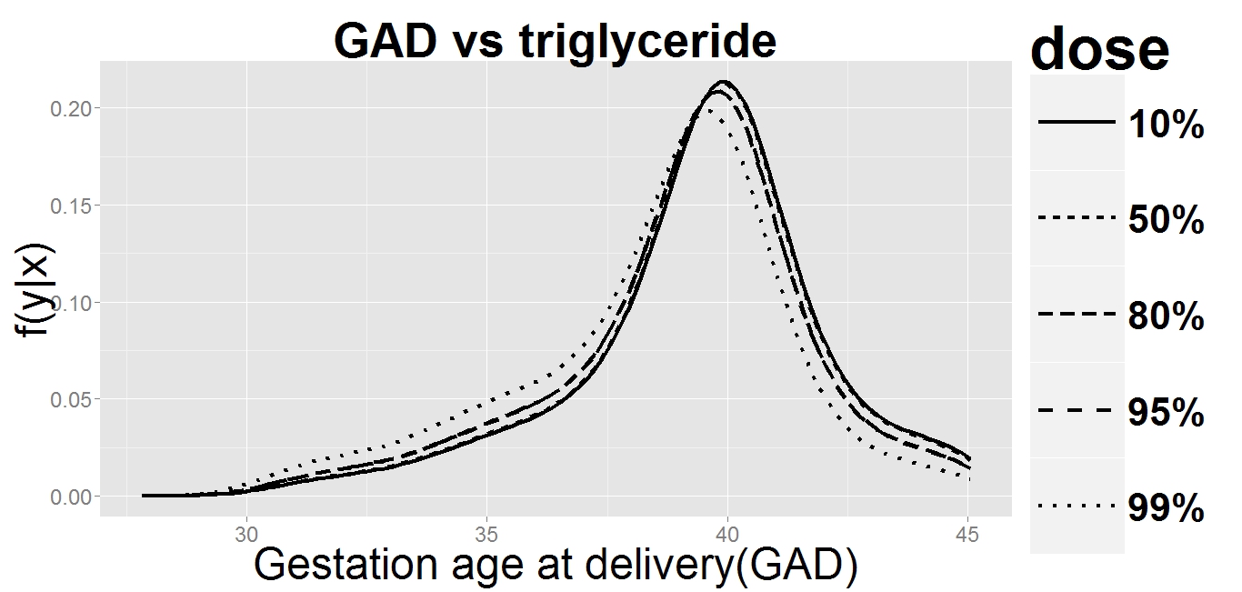
We study the Longnecker data to investigate the effect of varying levels of DDE on the distribution of GAD, focusing on the left tail of distribution to assess the effect on preterm births. In our study, following Dunson and Park (2008), we include only the 2313 subjects for whom the gestation age at delivery is less than 45 weeks, attributing higher values to measurement errors. We study the conditional density of GAD given different doses of DDE in the serum. We also study the effect of different levels of triglyceride on GAD. However, since DDE is a possible confounding factor, we conduct a bivariate analysis, including both DDE dose and triglyceride level as the covariates and study the effect on GAD at varying levels of one covariate, keeping the other fixed. We also investigate whether different levels of one covariate affect the distribution of the other.

Based on our findings, the very erratic behavior at locations where the DDE dose or triglyceride levels are 99th percentile is seen with some skepticism because of the sparsity of the data in that region. We notice an increasingly prominent peak near the left tail of GAD distribution with increasing dose of DDE, which agrees with the results of Longnecker et al. (2001) and Dunson and Park (2008), shown in the left panel of Figure 3. The right panel of Figure 3 suggests a tendency of higher risks of preterm birth at higher doses of triglycerides as well, though the difference was less pronounced.

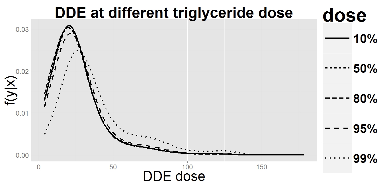
To investigate whether the results corresponding to triglycerides were confounded by the DDE doses, we first study the effect of triglyceride levels on DDE distribution and vice versa. Figure 4 shows that the distributions of the covariates are completely identical for varying levels of the other. The only exception is at 99th percentile of triglyceride for which the distribution of DDE doses seem to be shifted to the right. For fixed levels of triglyceride, increasing DDE doses shows an increasing left peak except where both DDE and triglyceride levels are very high, shown in Figure 5. For fixed doses of DDE the distribution of GAD at different levels of triglyceride do not follow any increasing trend and are almost indistinguishable from each other for all the different doses of DDE, as seen in Figure 6. This suggests that the increased risk of preterm birth can be attributed primarily to DDE doses, and there is no significant effect of different triglyceride levels on the gestation age. The apparent increasing risk of preterm birth for increasing level of triglycerides seen in the right panel of Figure 3 is mainly caused by DDE doses acting as a confounding factor.

Let $f_{1}$ and $f_{2}$ be two pdfs on $\mathscr{F}_{n}$ with corresponding cumulative distribution functions $F_{1}$ and $F_{2}$. Let $f_{p}$ be the initial density estimate on $\mathscr{F}_{p}$ such that $f_{p}$ is strictly positive and Lipschitz continuous with cumulative distribution function $F_{p}$. Let $\gamma_{1}={F_{p}}^{-1}\circ F_{1}$ and $\gamma_{2}={F_{p}}^{-1}\circ F_{2}$. Let $c_{1}=(c_{11},\ldots,c_{1k_{n}})^{{\mathrm{\scriptscriptstyle T}}}$ and $c_{2}=(c_{21},\ldots,c_{2k_{n}})^{{\mathrm{\scriptscriptstyle T}}}$ be the coefficients associated with the two elements of $T_{{\bf 1}}(\mathbb{S}_{\infty})$ corresponding to the tangent space representation of $\gamma_{1}$ and $\gamma_{2}$. Here $\mathscr{F}_{n}$ and $k_{n}$ are as introduced in section $2$ of the manuscript. Then the following Lemma bounds the norm difference of $f_{1}$ and $f_{2}$ with the norm difference in the coefficients.

References

- Abramson [1982] Ian S Abramson. On bandwidth variation in kernel estimates-a square root law. The annals of Statistics, pages 1217–1223, 1982.
- Bashtannyk and Hyndman [2001] David M Bashtannyk and Rob J Hyndman. Bandwidth selection for kernel conditional density estimation. Computational Statistics & Data Analysis, 36(3):279–298, 2001.
- Bhattacharya et al. [2010] A Bhattacharya, D Pati, and DB Dunson. Latent factor density regression models. Biometrika, 97(1):1–7, 2010.
- Birgé et al. [1998] Lucien Birgé, Pascal Massart, et al. Minimum contrast estimators on sieves: exponential bounds and rates of convergence. Bernoulli, 4(3):329–375, 1998.
- Chung and Dunson [2009] Yeonseung Chung and David B. Dunson. Nonparametric bayes conditional distribution modeling with variable selection. Journal of the American Statistical Association, 104(488):1646–1660, 2009. URL http://pubs.amstat.org/doi/abs/10.1198/jasa.2009.tm08302.
- De Carvalho [2011] Miguel De Carvalho. Confidence intervals for the minimum of a function using extreme value statistics. International Journal of Mathematical Modelling and Numerical Optimisation, 2(3):288–296, 2011.
- De Iorio et al. [2004] Maria De Iorio, Peter Muller, Gary L. Rosner, and Steven N. MacEachern. An anova model for dependent random measures. Journal of the American Statistical Association, 99(465):205–215, 2004. URL http://www.jstor.org/stable/27590366.
- Donoho et al. [1996] David L Donoho, Iain M Johnstone, Gérard Kerkyacharian, and Dominique Picard. Density estimation by wavelet thresholding. The Annals of Statistics, pages 508–539, 1996.
- Doosti and Hall [2016] Hassan Doosti and Peter Hall. Making a non-parametric density estimator more attractive, and more accurate, by data perturbation. Journal of the Royal Statistical Society: Series B (Statistical Methodology), 78(2):445–462, 2016.
- Dunson and Park [2008] David B Dunson and Ju-Hyun Park. Kernel stick-breaking processes. Biometrika, 95(2):307–323, 2008.
- Dunson et al. [2007] David B. Dunson, Natesh Pillai, and Ju-Hyun Park. Bayesian density regression. Journal of the Royal Statistical Society. Series B (Statistical Methodology), 69(2):pp. 163–183, 2007. ISSN 13697412. URL http://www.jstor.org/stable/4623261.
- Efromovich [2010] Sam Efromovich. Orthogonal series density estimation. Wiley Interdisciplinary Reviews: Computational Statistics, 2(4):467–476, 2010.
- Escobar and West [1995] Michael D Escobar and Mike West. Bayesian density estimation and inference using mixtures. Journal of the american statistical association, 90(430):577–588, 1995.
- Griffin and Steel [2006] J. E Griffin and M. F. J Steel. Order-based dependent dirichlet processes. Journal of the American Statistical Association, 101(473):179–194, 2006. URL http://pubs.amstat.org/doi/abs/10.1198/016214505000000727.
- Hall et al. [1991] Peter Hall, Simon J Sheather, MC Jones, and James Stephen Marron. On optimal data-based bandwidth selection in kernel density estimation. Biometrika, 78(2):263–269, 1991.
- Hansen [2004] Bruce E Hansen. Nonparametric conditional density estimation. Unpublished manuscript, 2004.
- Hjort and Glad [1995] Nils Lid Hjort and Ingrid K Glad. Nonparametric density estimation with a parametric start. The Annals of Statistics, pages 882–904, 1995.
- Hothorn et al. [2015] Torsten Hothorn, Lisa Möst, and Peter Bühlmann. Most likely transformations. arXiv preprint arXiv:1508.06749, 2015.
- Jain and Neal [2012] Sonia Jain and Radford M Neal. A split-merge markov chain monte carlo procedure for the dirichlet process mixture model. Journal of Computational and Graphical Statistics, 2012.
- Kalli et al. [2011] Maria Kalli, Jim E Griffin, and Stephen G Walker. Slice sampling mixture models. Statistics and computing, 21(1):93–105, 2011.
- Karunamuni and Zhang [2008] Rhoana J Karunamuni and Shunpu Zhang. Some improvements on a boundary corrected kernel density estimator. Statistics & Probability Letters, 78(5):499–507, 2008.
- Kundu and Dunson [2014] Suprateek Kundu and David B Dunson. Latent factor models for density estimation. Biometrika, 101(3):641–654, 2014.
- Lang [2012] Serge Lang. Fundamentals of differential geometry, volume 191. Springer Science & Business Media, 2012.
- Lenk [1988] Peter J Lenk. The logistic normal distribution for bayesian, nonparametric, predictive densities. Journal of the American Statistical Association, 83(402):509–516, 1988.
- Lenk [1991] Peter J Lenk. Towards a practicable bayesian nonparametric density estimator. Biometrika, 78(3):531–543, 1991.
- Leonard [1978] Tom Leonard. Density estimation, stochastic processes and prior information. Journal of the Royal Statistical Society. Series B (Methodological), pages 113–146, 1978.
- Lepski [2015] Oleg Lepski. Adaptive estimation over anisotropic functional classes via oracle approach. The Annals of Statistics, 43(3):1178–1242, 2015.
- Li and Racine [2007] Qi Li and Jeffrey Scott Racine. Nonparametric econometrics: theory and practice. Princeton University Press, 2007.
- Longnecker et al. [2001] Matthew P Longnecker, Mark A Klebanoff, Haibo Zhou, and John W Brock. Association between maternal serum concentration of the ddt metabolite dde and preterm and small-for-gestational-age babies at birth. The Lancet, 358(9276):110–114, 2001.
- MacEachern [1999] Steven N. MacEachern. Dependent nonparametric processes. ASA Proceedings of the Section on Bayesian Statistical Science, 1999. URL http://aima.eecs.berkeley.edu/~russell/classes/cs294/f05/papers/maceachern-1999.pdf.
- MacEachern and Müller [1998] Steven N MacEachern and Peter Müller. Estimating mixture of dirichlet process models. Journal of Computational and Graphical Statistics, 7(2):223–238, 1998.
- Marron and Wand [1992] J Steve Marron and Matt P Wand. Exact mean integrated squared error. The Annals of Statistics, pages 712–736, 1992.
- Müller et al. [1996] Peter Müller, Alaattin Erkanli, and MIKE West. Bayesian curve fitting using multivariate normal mixtures. Biometrika, 83(1):67–79, 1996.
- Norets and Pelenis [2012] Andriy Norets and Justinas Pelenis. Bayesian modeling of joint and conditional distributions. Journal of Econometrics, 168:332–346, 2012.
- Rosenblatt [1956] Murray Rosenblatt. Remarks on some nonparametric estimates of a density function. The Annals of Mathematical Statistics, 27(3):832–837, 1956.
- Saoudi et al. [1994] S Saoudi, A Hillion, and F Ghorbel. Non–parametric probability density function estimation on a bounded support: Applications to shape classification and speech coding. Applied Stochastic models and data analysis, 10(3):215–231, 1994.
- Saoudi et al. [1997] S Saoudi, F Ghorbel, and A Hillion. Some statistical properties of the kernel-diffeomorphism estimator. Applied stochastic models and data analysis, 13(1):39–58, 1997.
- Sheather and Jones [1991] Simon J Sheather and Michael C Jones. A reliable data-based bandwidth selection method for kernel density estimation. Journal of the Royal Statistical Society. Series B (Methodological), pages 683–690, 1991.
- Srivastava and Klassen [2016] Anuj Srivastava and Eric P Klassen. Functional and shape data analysis. Springer, 2016.
- Tabak and Turner [2013] EG Tabak and Cristina V Turner. A family of nonparametric density estimation algorithms. Communications on Pure and Applied Mathematics, 66(2):145–164, 2013.
- Tabak and Trigila [2014] Esteban G Tabak and Giulio Trigila. Data-driven optimal transport. Commun. Pure. Appl. Math. doi, 10:1002, 2014.
- Terrell and Scott [1992] George R Terrell and David W Scott. Variable kernel density estimation. The Annals of Statistics, pages 1236–1265, 1992.
- Tokdar [2007] Surya T Tokdar. Towards a faster implementation of density estimation with logistic gaussian process priors. Journal of Computational and Graphical Statistics, 16(3):633–655, 2007.
- Tokdar et al. [2010] Surya T Tokdar, Yu M Zhu, Jayanta K Ghosh, et al. Bayesian density regression with logistic gaussian process and subspace projection. Bayesian analysis, 5(2):319–344, 2010.
- Triebel [2006] Hans Triebel. Theory of function spaces. iii, volume 100 of monographs in mathematics. BirkhauserVerlag, Basel, 2006.
- Turnbull and Ghosh [2014] Bradley C Turnbull and Sujit K Ghosh. Unimodal density estimation using bernstein polynomials. Computational Statistics & Data Analysis, 72:13–29, 2014.
- Van Kerm [2003] Philippe Van Kerm. Adaptive kernel density estimation. Stata Journal, 3(2):148–156, 2003.
- Vermehren and de Oliveira [2015] V Vermehren and HM de Oliveira. Close expressions for meyer wavelet and scale function. arXiv preprint arXiv:1502.00161, 2015.
- Wong and Shen [1995] Wing Hung Wong and Xiaotong Shen. Probability inequalities for likelihood ratios and convergence rates of sieve mles. The Annals of Statistics, pages 339–362, 1995.
Florida State University
E-mail: (s.dasgupta@stat.fsu.edu)
Texas A&M University
E-mail: (debdeep@stat.tamu.edu)
E-mail: (anuj@stat.fsu.edu)