$L^{p}$ almost conformal isometries of Sub-Semi-Riemannian metrics and Solvability of a Ricci equation

The goal of this note is to prove that the two principal results of D. DeTurck [11] given for positive definite symmetric bilinear form and for special Einstein metrics can be extended significantly in different ways.

Firstly, we can extend the positive definideness condition of the Riemannian metrics to Sub-Semi-Riemmannian metrics with the same rank and signature.

Secondly we are able to replace some particular Einstein metrics of non zero scalar curvature by any parallel Ricci metrics (ie. metrics with covariantly constant Ricci tensor).

Let $M$ be a smooth compact manifold without boundary. A Sub-Semi-Riemannian metric $\mathfrak{G}$ (SSR-metric for short) is a symmetric covariant 2-tensor field with constant signature and constant rank.

Let us now state the first result, interesting by itself, about almost conformal isometries.

Before going to the application for a Ricci equation, let us introduce some notations. For $(M,{{\mathfrak{g}}})$ a smooth riemannian manifold, we denote by $\operatorname{Ric}({{\mathfrak{g}}})$ its Ricci curvature. For a real constant $\Lambda$, we consider the operator

This operator is geometric in the sense that for any smooth diffeomorphism $\varphi$,

We would like to invert $\operatorname{Ein}$. We thus choose $\mathcal{E}$ a symmetric 2-tensor field on $M$, and look for ${{\mathfrak{g}}}$ Riemannian metric such that

This is a geometrically natural and difficult quasilinear system to solve, already for perturbation methods. The prescribed Ricci curvature problem has a long history starting with the work of D. DeTurck [9],[11], [10], [13], [12], [1], [14], [2], [3], [6],[8], [7], [5], [4],…

Motivated by the explosion of studies around the Ricci flow, and recently, some discrete versions thereof (eg. $\operatorname{Ein}(g_{i+1})=g_{i}$), a renewed interest arises for this kind of natural geometric equations. We invite the reader to look at the nice recent works of A. Pulemotov and Y. Rubinstein [16] and [17] for related results. Our contribution here is the following.

The proof goes by combining the Lemma 1.1 , the local inversion result of Proposition 3.1 for weak regular metric (where the conformal factor $f$ is not required) and a regularity argument. We have then solved the problem up to a positive function $f$. Here we do not expect that $f$ can be taken equals to one in general, this will be the subject of future investigations.

Parallel Ricci metrics, are (locally) products of Einstein metrics (see eg. [18]). They exists on the simplest examples of manifolds who do not admit Einstein metrics, like $\mathbb{S}^{1}\times\mathbb{S}^{2}$, $\Sigma_{g}\times\mathbb{S}^{2},$ ($g\geq 1$) or $\Sigma_{g}\times\mathbb{T}^{2},$ ($g\geq 2$) where $\Sigma_{g}$ is a surface of genius $g$. They are also static solutions of some geometric fourth order flows (eg. $\partial_{t}g=\Delta_{g}\operatorname{Ric}(g)$). Finally they are particular cases of Riemannian manifolds with Harmonic curvature (or equivalently Codazzi Ricci tensor).

Our global result show once again that such metrics with covariantly constant Ricci tensor deserve a particular attention.

Acknowledgments : I am grateful to Philippe Delanoë for comments and improvements, and to Alexandra Barbieri and François Gautero for the picture of the simplex.

We follow the section 3 called ”approximation lemma” in [11] in order to verify that all the step there can be adapted for SSR-metrics as above. This will prove the Lemma 1.1.

We will keep almost the same notations as in [11], just replacing $S$ and $R$ there respectively by $\mathfrak{G}$ and $\mathcal{G}$ here.

Let $\mathfrak{G}$ and $\mathcal{G}$ be as in the introduction, we thus assume they have the same signature and the same rank. For the rest of the section we fix a Riemannian metric $g$, an $\varepsilon>0$ and $p\in[1,+\infty)$. All the measures, volumes, and norms are understood with respect to $g$.

At each point $x\in M$, the two SSR-metric $\mathfrak{G}$ and $\mathcal{G}$ having the same rank and signature, there exists an orientation preserving automorphism $u_{x}$ of $T_{x}M$, such that

For $x\in M$, the following construction can be performed using the $g$-exponential map at $x$. There exists an open set $U_{x}$ such that :

Let $\Omega$, $\Omega_{1}$, $\Omega_{2}$, $\Omega_{3}$ be some open neighbourhoods of the $(n-1)$ dimensional skeleton (composed with union of the boundary of all simplex) with the properties :

and

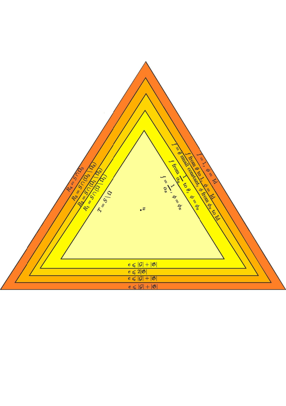
The rest of the proof in section 3 of [11] is based on triangular inequalities between norms of tensors and can be implemented here without any change. For a better understanding, though, we provide further details of the figure page 368 of [11], specifying the estimates that occur on the differents parts of the simplex, see figure 1. On the picture, we have denoted the error $|\Phi^{*}(f\mathcal{G})-\mathfrak{G}|$ by $e$ :

On the inner part $T$ of the simplex, $e$ is estimated by (2.1). The transition of the diffeomorphism $\Phi$, on the middle ring $R_{2}=S\cap(\Omega_{1}\backslash\Omega_{2})$, from $\Phi_{x}$ to the identity, still exist because our $\Phi_{x}=\sqrt{\alpha_{x}}\,u_{x}$ is an orientation preserving map with norm less than 1 as in [11].

We revisit the section 2 of [11] called “perturbation lemma”.

We first need to introduce some operators. The divergence of a symmetric 2-tensor field and its $L^{2}$ adjoint acting on one form are

The gravitationnal operator acting on symmetric 2-tensors is

The Lichnerowicz Laplacian is ²² 2 Different sign convention with DeTurck

It appears in the Linearization of the Ricci operator :

The Hodge Laplacian acting on one forms is

We also define the following Laplacian

We denote by $V$ its finite dimensionnal kernel, composed of smooth one forms (by elliptic regularity).

We start with the equivalent of proposition 2.1 in [11].

In [11], the proof of the corresponding proposition is given by a succession of lemmas. We thus revisit them one after the other. Some care is needed because we have to replace Ric and $-\Delta_{L}$ there, respectively with Ein and $\Delta_{L}+2\Lambda$ here. Furthermore, in our context, the operator $\Delta_{L}+2\Lambda$ has no kernel whereas the kernel of $\Delta_{L}$ is nonempty in [11], spanned by $g$. We clearly have also for any Riemannian metrics $g$, the Bianchi identity

We start with a local study of the action of the diffeomorphim group on the covariant symetrics 2-tensors, near a non degenerate parallel one. The result obtained remains in the spirit of the local study near a Riemmanian metric by Berger, Ebin, or Palais (see eg. the lemma 2.3 of [11]). Here the metric tensor is replaced by a non degenerate parallel tensor field.

Let us recall the lemma 2.5 in [11] :⁴⁴ 4 It seems there is a misprint in the proof this lemma: The Ricci term for $\delta G\delta^{*}$ at the top of page 362 in [11] has a different sign.

The equivalent of the lemma 2.6 in [11] becomes (we do not have to quotient by $R\,g$ because of no kernel for us, and so we do not need to adjust with a constant $c$).

From the Lemma 3.2 with $E=\operatorname{Ein}({g})$ and Lemma 3.4 we directly deduce :

We will complete the proof of proposition 3.1, where now ${\mathcal{E}}\in H^{k+1,p}$, but ${{\mathfrak{g}}}$ and $\varphi$ still cames from Lemma 3.5 so $\varphi$ is a priori not regular enough. If we inspect the pages 364-365 in [11] we can see that we just have to change $\operatorname{Ric}({{\mathfrak{g}}})$ by $\operatorname{Ein}({{\mathfrak{g}}})$ to obtain that $\varphi$ is in fact in $H^{k+2,p}$. We conclude that $(\varphi^{-1})^{*}{{\mathfrak{g}}}\in H^{k+1,p}$ and has ${\mathcal{E}}$ as its image by $\operatorname{Ein}$. At this level we also use that $\operatorname{Ein}({{\mathfrak{g}}})$ is non degenerate (see equation (2.8) there).

The Theorem 1.2 is now a direct consequence of the Lemma 1.1, the Proposition 3.1 with $k=0$, and the regularity result of [12].

References

- [1] Alfred Baldes, Nonexistence of Riemannian metrics with prescribed Ricci tensor, Nonlinear problems in geometry (Mobile, Ala., 1985), Contemp. Math., vol. 51, Amer. Math. Soc., Providence, RI, 1986, pp. 1–8. MR 848927 (87k:53085)
- [2] Ph. Delanoë, Obstruction to prescribed positive Ricci curvature, Pacific J. Math. 148 (1991), no. 1, 11–15.
- [3] by same author, Local solvability of elliptic, and curvature, equations on compact manifolds, J. Reine Angew. Math. 558 (2003), 23–45. MR 1979181 (2004e:53054)
- [4] E. Delay, Inversion d’opérateurs de courbure au voisinage de la métrique euclidiennne, bull. Soc. Math. France, à paraître, hal-00973138.
- [5] by same author, Sur l’inversion de l’opérateur de Ricci au voisinage d’une métrique Ricci parallèle, Annales de l’institut Fourier, à paraître, hal-00974707v2.
- [6] by same author, Etude locale d’opérateurs de courbure sur l’espace hyperbolique, J. Math. Pures Appli. 78 (1999), 389–430.
- [7] by same author, Study of some curvature operators in the neighbourhood of an asymptotically hyperbolic Einstein manifold, Advances in Math. 168 (2002), 213–224.
- [8] E. Delay and M. Herzlich, Ricci curvature in the neighbourhood of rank-one symmetric spaces, J. Geometric Analysis 11 (2001), no. 4, 573–588.
- [9] D. DeTurck, Existence of metrics with prescribed ricci curvature : Local theory, Invent. Math. 65 (1981), 179–207.
- [10] Dennis DeTurck and Hubert Goldschmidt, Metrics with prescribed Ricci curvature of constant rank. I. The integrable case, Adv. Math. 145 (1999), no. 1, 1–97.
- [11] Dennis M. DeTurck, Prescribing positive Ricci curvature on compact manifolds, Rend. Sem. Mat. Univ. Politec. Torino 43 (1985), no. 3, 357–369 (1986).
- [12] Dennis M. DeTurck and J. Kazdan, Some regularity theorems in riemannian geometry, Ann. Scient. Ec. Norm. Sup. 14 (1981), no. 4, 249–260.
- [13] Dennis M. DeTurck and Norihito Koiso, Uniqueness and nonexistence of metrics with prescribed Ricci curvature, Ann. Inst. H. Poincaré Anal. Non Linéaire 1 (1984), no. 5, 351–359.
- [14] Richard Hamilton, The Ricci curvature equation, Seminar on nonlinear partial differential equations (Berkeley, Calif., 1983), Math. Sci. Res. Inst. Publ., vol. 2, Springer, New York, 1984, pp. 47–72. MR 765228 (86b:53040)
- [15] A. Lichnerowicz, Propagateurs et commutateurs en relativité générale, Pub. Math. de l’IHES 10 (1961), 5–56.
- [16] A. Pulemotov, Metrics with prescribed Ricci curvature near the boundary of a manifold, Mathematische Annalen 357 (2013), 969–986.
- [17] A. Pulemotov and Y.A. Rubinstein, Ricci iteration on homogeneous spaces, arXiv:1606.05064 [math.DG] (2016).
- [18] H. Wu, Holonomy groups of indefinite metrics, Pacific J. Math. 20 (1967), 351–392.