跳到论文正文
W Papers独立论文阅读器 arXiv:1701.05247 论文正文 计算阅读时间 · 0%
引用这篇论文根据当前论文元数据生成,正式投稿前建议核对。


License: arXiv.org perpetual non-exclusive license
arXiv:1701.05247v2 [cs.IT] 24 Jan 2017

Downlink Non-Orthogonal Multiple Access with Limited FeedbackThanks: X. Liu, H. Jafarkhani are with Center for Pervasive Communications & Computing, University of California, Irvine, Irvine, CA 92697–2625 USA (Email: {xiaoyil3, hamidj}@uci.edu).

Xiaoyi (Leo) Liu, Student Member, IEEE, Hamid Jafarkhani, Fellow, IEEE Affiliation: 
Abstract

In this paper, we analyze downlink non-orthogonal multiple access (NOMA) networks with limited feedback. Our goal is to derive appropriate transmission rates for rate adaptation and minimize outage probability of minimum rate for the constant-rate data service, based on distributed channel feedback information from receivers. We propose an efficient quantizer with variable-length encoding that approaches the best performance of the case where perfect channel state information is available everywhere. We prove that in the typical application with two receivers, the losses in the minimum rate and outage probability decay at least exponentially with the minimum feedback rate. We analyze the diversity gain and provide a sufficient condition for the quantizer to achieve the maximum diversity order. For NOMA with KK receivers where K>2K>2, we solve the minimum rate maximization problem within an accuracy of ϵ\epsilon in time complexity of O⁡(K​log⁡1ϵ)O\left(K\log\frac{1}{\epsilon}\right), then, we apply the previously proposed quantizers for K=2K=2 to the case of K>2K>2. Numerical simulations are presented to demonstrate the efficiency of our proposed quantizers and the accuracy of the analytical results.

Index Terms: 
NOMA, rate adaptation, outage probability, minimum rate, limited feedback

I Introduction

Non-orthogonal multiple access (NOMA) has received significant attention recently for its superior spectral efficiency [1]. It is a promising candidate for mobile communication networks, and has been included in LTE Release 13 for the scenario of two-user downlink transmission under the name of multi-user superposition transmission [2]. The key idea of NOMA is to multiplex multiple users with superposition coding at different power levels, and utilize successive interference cancellation (SIC) at receivers with better channel conditions. Specifically, for NOMA with two receivers, the messages to be sent are superposed with different power allocation coefficients at the BS side. At the receivers’ side, the weaker receiver decodes its intended message by treating the other’s as noise, while the stronger receiver first decodes the message of the weaker receiver, and then decodes its own by removing the other message from the received signal. In this way, the weaker receiver benefits from larger power, and the stronger receiver is able to decode its own message with no interference. Hence, the overall performance of NOMA is enhanced, compared with traditional orthogonal multiple access schemes. It is shown in [3] that the rate region of NOMA is the same as the capacity region of Gaussian broadcast channels with two receivers, but with an additional constraint that the stronger receiver is assigned less power than the weaker one.

There has been a lot of work on NOMA. In [1] and [3], the authors evaluated the benefits of downlink NOMA from the system and information theoretic perspectives, respectively. NOMA with multiple antennas was studied in [4]. A lot of effort has been put into the power allocation design in NOMA. For example, the authors in [5] and [6] analyzed the necessary conditions for NOMA with two users to beat the performance of time-division-multiple-access (TDMA), and derived closed-form expressions for the expected data rates and outage probabilities. In [7], power allocation based on proportional fairness scheduling was investigated for downlink NOMA. Transmit power minimization subject to rate constraints was discussed in [8].

However, all the mentioned work on NOMA has assumed a perfect knowledge of the distributed channel state information (CSI) at the BS and all the geographically-distributed receivers, which is difficult to realize in practice. Therefore, we consider the limited feedback scenario wherein each receiver only has access to its own local CSI from the BS to itself, and then broadcasts its feedback information to the BS and other receivers [9, 10]. Under such settings, interesting problems arise, for example: How to design simple but efficient quantizers for NOMA? What are the performance losses compared with the full-CSI case? A user-selection scheme based on limited feedback was studied in [11]. In [12], the authors proposed a one-bit feedback scheme for ordering users in downlink Massive-MIMO-NOMA systems, and derived the achieved outage probability. In [13], the authors derived the outage probability of NOMA based on one-bit feedback of channel quality from each receiver, and performed power allocation to minimize the outage probability. Additionally, the problems of transmit power minimization and user fairness maximization based on statistical CSI subject to outage constraints were studied in [14]. In [15], the authors derived the outage probability and sum rate with fixed power allocation by assuming imperfect and statistical CSI.

In this paper, we focus on the limited feedback design for the typical scenario of downlink NOMA, where a BS communicates with two receivers simultaneously [2]. Based on distributed feedback and in the interest of user fairness, we wish to have the minimum rate of the receivers be as large as possible. To dynamically adjust the transmission rates for better channel utilization, we propose a uniform quantizer which assigns each value to its left boundary point and employs variable-length encoding (VLE). Then, power allocation is calculated based on the channel feedback. We calculate the transmission rates that can be supported by the current channel states, and analyze the rate loss compared with the full-CSI scenario. The derived upper bound on rate loss shows that it decreases at least exponentially with the minimum of the feedback rates. For the constant-rate service where outage probability is the main concern, we conversely propose a uniform quantizer which quantizes each value to its right boundary point. Through the developed upper bound, we show the outage probability loss also decays at least exponentially with the minimum of feedback rate. Additionally, we analyze the achieved diversity gain and provide a sufficient condition on the proposed quantizer in order to achieve the full-CSI diversity order. For the general scenario with KK receivers, we solve the minimum rate maximization problem within an accuracy of ϵ\epsilon in time complexity of O⁡(K​log⁡1ϵ)O\left(K\log\frac{1}{\epsilon}\right), and apply the previously proposed quantizers for the two-user case here by treating the quantized channels as the perfect ones. We perform Monte Carlo numerical simulations to verify the superiority of our proposed quantizers and the accuracy of the theoretical analysis.

The primary goal of this paper is to study the impacts of quantization on the performance of NOMA, and provide meaningful insights for practical limited feedback design. To summarize, the main contributions of this paper are three-fold:

  1. (1)

    We propose efficient quantizers to maximize the minimum rate in NOMA. The ideas of our proposed quantizers and VLE as well as the designs for rate adaptation and outage probability based on distributed feedback can be generalized to many other scenarios, e.g., NOMA with other performance measures, the more general interference channels, and so on.

  2. (2)

    Our theoretical analysis serves as a general framework to analyze the performances of such quantizers in NOMA and other scenarios. For instance, it can be easily applied to study the performances of other power allocation schemes in NOMA based on limited feedback, i.e., [5, 6].

  3. (3)

    We solve the minimum rate maximization problem for any number of receivers with linear time complexity.

The remainder of this paper is organized as follows: In Section II, we provide a brief description of the system model and formulate the problem of limited feedback. In Sections III and IV, we propose efficient quantizers for rate adaptation and outage probability, and analyze the performance loss. We extend our proposed quantizers to the general case with any number of receivers in Section V. Numerical simulations are provided in Section VI. We draw the main conclusions and summarize future work in Section VII. Technical proofs are presented in the appendices.

Notations: The sets of real and natural numbers are represented by ℛ\mathpzc{R} and 𝒩\mathpzc{N}, respectively. For any x∈ℛx\in\mathpzc{R}, ⌊x⌋\lfloor x\rfloor is the largest integer that is less than or equal to x, and ⌈x⌉\lceil x\rceil is the smallest integer that is larger than or equal to xx. Pr​{⋅}\text{Pr}\{\cdot\} and 𝙴⁡[⋅]\mathtt{E}[\cdot] represent the probability and expectation, respectively. For a random variable (r.v.) XX, fX​(⋅)f_{X}(\cdot) is its probability density function (p.d.f.). ℂ​ℕ​(μ,λ)\mathbbmss{CN}(\mu,\lambda) represents a circularly symmetric complex Gaussian r.v. with mean μ\mu and variance λ\lambda. For a logical statement 𝚂𝚃\mathtt{ST}, we let 𝟏𝚂𝚃=1{\boldsymbol{1}}_{\rm\mathtt{ST}}=1 when 𝚂𝚃\mathtt{ST} is true, and 𝟏𝚂𝚃=0{\boldsymbol{1}}_{\rm\mathtt{ST}}=0 otherwise. Finally, the expression X∼YZX\sim_{Y}Z means 0<limY→∞XZ<∞0<\lim_{Y\rightarrow\infty}\frac{X}{Z}<\infty.

II Problem Formulation

II-A System Model
Refer to caption
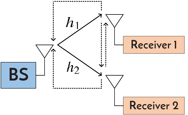
Fig. 1: Downlink NOMA networks. The solid and dashed lines represent the signal and feedback links, respectively.

Consider the downlink transmission in Fig. 1, where a BS is to transmit a superposition of two symbols to two receivers over the same resource block. Both BS and receivers are equipped with only a single antenna. According to the multiuser superposition transmission scheme [2], the transmitted signal is formed as

x=P1​s1+P2​s2,\displaystyle x=\sqrt{P_{1}}s_{1}+\sqrt{P_{2}}s_{2},

where sis_{i} is the information bearing symbol for Receiver ii with 𝙴⁡[si]=0\mathtt{E}\left[s_{i}\right]=0 and 𝙴⁡[|si|2]=1\mathtt{E}\left[\left|s_{i}\right|^{2}\right]=1 for each channel state (the expectation is over all transmitted symbols); PiP_{i} is the average transmit power associated with sis_{i}. Let P=P1+P2P=P_{1}+P_{2} be the total transmit power, and α=P1P\alpha=\frac{P_{1}}{P} be the power allocation coefficient, then, P1=α​PP_{1}=\alpha P and P2=(1−α)​PP_{2}=(1-\alpha)P with 0≤α≤10\leq\alpha\leq 1.

Denote by hi∼ℂ​ℕ​(0,λi)h_{i}\sim\mathbbmss{CN}(0,\lambda_{i}) the channel coefficient from the BS to Receiver ii. Without loss of generality, assume λ1≥λ2\lambda_{1}\geq\lambda_{2}. The received signals at Receivers 1 and 2 are respectively given by

y1=h1​P1​s1+h1​P2​s2+n1,y2=h2​P1​s1+h2​P2​s2+n2,\displaystyle y_{1}=h_{1}\sqrt{P_{1}}s_{1}+h_{1}\sqrt{P_{2}}s_{2}+n_{1},\quad y_{2}=h_{2}\sqrt{P_{1}}s_{1}+h_{2}\sqrt{P_{2}}s_{2}+n_{2},

where ni∼ℂ​ℕ​(0,1)n_{i}\sim\mathbbmss{CN}(0,1) represents the background noise. Let Hi=|hi|2H_{i}=\left|h_{i}\right|^{2}, then, the p.d.f. of HiH_{i} is fHi​(x)=e−λixλif_{H_{i}}(x)=\frac{e^{-\frac{\lambda_{i}}{x}}}{\lambda_{i}} for x>0x>0.11 1 The results in this paper can be trivially generalized to other distributions of H1H_{1} and H2H_{2}. We assume a quasi-static channel model, in which the channels vary independently from one block to another, while remaining constant within each block. Either receiver is assumed to perfectly estimate its local CSI (i.e., HiH_{i}), and send the associated quantized local CSI to the other receiver and the BS in a broadcast manner via error-free and delay-free feedback links [16, 17].

With SIC, the stronger receiver with better channel condition (i.e., larger HiH_{i}) first decodes the message for the weaker receiver, and then decodes its own after removing the message of the weaker one from its received signal; the weaker receiver with poorer channel condition directly decodes its own message by treating the message of the stronger one as noise [18, 19]. Specifically, when H1≥H2H_{1}\geq H_{2}, the rate for Receiver 2 (i.e., the weaker one) to decode s2s_{2} by treating s1s_{1} as noise is

r2​(α)=log2⁡(1+P​H2​(1−α)α​H2​P+1),\displaystyle r_{2}(\alpha)=\log_{2}\left(1+\frac{PH_{2}(1-\alpha)}{\alpha H_{2}P+1}\right),

which is not larger than the rate for Receiver 1 to decode s2s_{2}, given as r1→2=log2⁡(1+P​H1​(1−α)α​H1​P+1)r_{1\rightarrow 2}=\log_{2}\left(1+\frac{PH_{1}(1-\alpha)}{\alpha H_{1}P+1}\right). If s2s_{2} is transmitted at the rate of r2​(α)r_{2}(\alpha), Receiver 1 can decode s2s_{2} successfully with an arbitrarily small probability of error [20]. Afterwards, Receiver 1 can remove h1​P2​s2h_{1}\sqrt{P_{2}}s_{2} from y1y_{1}, and achieve a data rate for s1s_{1} as

r1​(α)\displaystyle r_{1}(\alpha) =log2⁡(1+α​P​H1).\displaystyle=\log_{2}\left(1+\alpha PH_{1}\right).

On the other hand, when H1<H2H_{1}<H_{2}, Receiver 2 first decodes s1s_{1}, removes h2​P1​s1h_{2}\sqrt{P_{1}}s_{1} from y2y_{2}, and then decodes s2s_{2}, while Receiver 1 decodes s1s_{1} directly by treating s2s_{2} as noise.

II-B Maximum Minimum Rate

Our goal is to maximize the minimum of r1​(α)r_{1}(\alpha) and r2​(α)r_{2}(\alpha) to ensure fairness between receivers [10, 21]. When perfect CSI is available at the BS and receivers, the optimal power allocation coefficient α⋆\alpha^{\star} can be found by solving the optimization problem rmax=max0≤α≤1⁡min⁡{r1​(α),r2​(α)}r_{\max}=\max\limits_{0\leq\alpha\leq 1}\min\{r_{1}(\alpha),r_{2}(\alpha)\}, the solution of which is given in the following theorem.

Theorem 1.

When H1≥H2H_{1}\geq H_{2}, the solution of max0≤α≤1⁡min⁡{r1​(α),r2​(α)}\max\limits_{0\leq\alpha\leq 1}\min\{r_{1}(\alpha),r_{2}(\alpha)\} is given by

α⋆=2​H2(H1+H2)2+4​H1​H22​P+(H1+H2).\displaystyle\alpha^{\star}=\frac{2H_{2}}{\sqrt{\left(H_{1}+H_{2}\right)^{2}+4H_{1}H_{2}^{2}P}+\left(H_{1}+H_{2}\right)}. (1)
Proof.

Notice that with α\alpha increasing from 00 to 11, r1​(α)r_{1}(\alpha) increases from 0 to log2⁡(1+P​H1)\log_{2}\left(1+PH_{1}\right) and r2​(α)r_{2}(\alpha) decreases from log2⁡(1+P​H2)\log_{2}\left(1+PH_{2}\right) to 00. Since log2⁡(1+P​H1)≥log2⁡(1+P​H2)\log_{2}\left(1+PH_{1}\right)\geq\log_{2}\left(1+PH_{2}\right), the maximum minimum rate is reached when r1​(α⋆)=r2​(α⋆)r_{1}(\alpha^{\star})=r_{2}(\alpha^{\star}), from which α⋆\alpha^{\star} in (1) is derived.  

The expression of α⋆\alpha^{\star} when H1<H2H_{1}<H_{2} can be obtained straightforwardly. It is found from (1) that: (i) Both messages attain the same rate at optimality, i.e., r1​(α⋆)=r2​(α⋆)=rmaxr_{1}\left(\alpha^{\star}\right)=r_{2}\left(\alpha^{\star}\right)=r_{\max}. Moreover, it can be verified that the rate pair (r1​(α⋆),r2​(α⋆))(r_{1}\left(\alpha^{\star}\right),r_{2}\left(\alpha^{\star}\right)) is on the rate region boundaries of both NOMA and Gaussian broadcast channels with two receivers [3]. (ii) When P→0P\rightarrow 0, α⋆→H2H1+H2\alpha^{\star}\rightarrow\frac{H_{2}}{H_{1}+H_{2}}, in which case the power assigned to the stronger receiver is in proportion to the channel quality of the weaker one; when P→∞P\rightarrow\infty, α⋆→0\alpha^{\star}\rightarrow 0, then, BS should allocate almost all the power to the weaker one. (iii) α⋆≥12\alpha^{\star}\geq\frac{1}{2}. Generally, NOMA steers more power towards the weaker receiver to balance their transmissions.

It is also worth pointing out that α⋆\alpha^{\star} in (1) satisfies the requirement for power allocation considered in [6] and [5]: the achieved individual rate should exceed that in the TDMA scheme, i.e., ri​(α⋆)≥12​log2⁡(1+P​Hi)r_{i}(\alpha^{\star})\geq\frac{1}{2}\log_{2}(1+PH_{i}) for i=1,2i=1,2. Therefore, the maximum minimum rate we consider in this paper achieves higher rates in addition to better fairness between receivers.

With perfect CSI, the decoding order is determined based on whether H1≥H2H_{1}\geq H_{2} holds. The maximum minimum rate is

rmax\displaystyle r_{\max} ={log2⁡(1+2​H1​H2​P(H1+H2)2+4​H1​H22​P+(H1+H2)),H1≥H2,log2⁡(1+2​H1​H2​P(H1+H2)2+4​H12​H2​P+(H1+H2)),H1<H2,\displaystyle=\left\{\begin{matrix}\log_{2}\left(1+\frac{2H_{1}H_{2}P}{\sqrt{\left(H_{1}+H_{2}\right)^{2}+4H_{1}H_{2}^{2}P}+\left(H_{1}+H_{2}\right)}\right),&H_{1}\geq H_{2},\\ \log_{2}\left(1+\frac{2H_{1}H_{2}P}{\sqrt{\left(H_{1}+H_{2}\right)^{2}+4H_{1}^{2}H_{2}P}+\left(H_{1}+H_{2}\right)}\right),&H_{1}<H_{2},\\ \end{matrix}\right. (2)

and the outage probability of minimum rate is

𝚘𝚞𝚝min=Pr{rmax<rth},\displaystyle\mathtt{out}_{\min}=\text{Pr}\left\{r_{\max}<r_{\rm th}\right\}, (3)

where rthr_{\rm th} is the data rate at which the BS will transmit s1s_{1} and s2s_{2} for every channel state.

II-C Limited Feedback

In the limited-feedback scenario, for an arbitrary quantizer q:ℛ→ℛq:\mathpzc{R}\rightarrow\mathpzc{R}, Receiver ii maps HiH_{i} to q⁡(Hi)q\left(H_{i}\right), and feeds the index of q⁡(Hi)q\left(H_{i}\right) back to the BS and the other receiver, as shown in Fig.1. The index of q⁡(Hi)q\left(H_{i}\right) is decoded and the value of q⁡(Hi)q\left(H_{i}\right) is recovered. The decoding order will be contingent on whether q⁡(H1)≥q⁡(H2)q\left(H_{1}\right)\geq q\left(H_{2}\right). For instance, when q⁡(H1)≥q⁡(H2)q(H_{1})\geq q(H_{2}), Receiver 1 is considered “stronger”, while Receiver 2 is “weaker”. In this case, the power allocation coefficient is computed based on (1) by treating q⁡(Hi)q\left(H_{i}\right) as HiH_{i}, i.e., αq=2​q​(H2)(q⁡(H1)+q⁡(H2))2+4​q​(H1)​q2​(H2)​P+q⁡(H1)+q⁡(H2)\alpha_{q}=\frac{2q(H_{2})}{\sqrt{\left(q(H_{1})+q(H_{2})\right)^{2}+4q(H_{1})q^{2}(H_{2})P}+q(H_{1})+q(H_{2})}.

For rate adaptation, we shall design appropriate rates r1,qr_{1,q} and r2,qr_{2,q} for the messages s1s_{1} and s2s_{2} based on limited feedback from the two receivers, such that r1,qr_{1,q} and r2,qr_{2,q} can be supported and NOMA can be performed. The corresponding rate loss will be

rloss=rmax−min⁡{r1,q,r2,q},\displaystyle r_{\rm loss}=r_{\max}-\min\left\{r_{1,q},r_{2,q}\right\},

where rmaxr_{\max} is given in (2).

For a constant-rate service, we care more about whether the current channels are strong enough to support target data rate with the power allocation coefficient computed based on limited feedback. The achieved outage probability is 𝚘𝚞𝚝q=Pr{rq<rth}\mathtt{out}_{q}=\text{Pr}\left\{r_{q}<r_{\rm th}\right\}, where

rq\displaystyle r_{q} =min⁡{r1​(αq),r2​(αq)}\displaystyle=\min\left\{r_{1}\left(\alpha_{q}\right),r_{2}\left(\alpha_{q}\right)\right\}
={min⁡{log2⁡(1+P×αq×H1),log2⁡(1+P​H2​(1−αq)P​H2​αq+1)},q⁡(H1)≥q⁡(H2),min⁡{log2⁡(1+P​H1​(1−αq)P​H1​αq+1),log2⁡(1+P×αq×H2)},q⁡(H1)<q⁡(H2),\displaystyle=\left\{\begin{matrix}\min\left\{\log_{2}\left(1+P\times\alpha_{q}\times H_{1}\right),\log_{2}\left(1+\frac{PH_{2}\left(1-\alpha_{q}\right)}{PH_{2}\alpha_{q}+1}\right)\right\},&q(H_{1})\geq q(H_{2}),\\ \min\left\{\log_{2}\left(1+\frac{PH_{1}\left(1-\alpha_{q}\right)}{PH_{1}\alpha_{q}+1}\right),\log_{2}\left(1+P\times\alpha_{q}\times H_{2}\right)\right\},&q(H_{1})<q(H_{2}),\end{matrix}\right.

The outage probability loss is given as

𝚘𝚞𝚝loss,q=𝚘𝚞𝚝min−𝚘𝚞𝚝q.\displaystyle\mathtt{out}_{{\rm loss},q}=\mathtt{out}_{\min}-\mathtt{out}_{q}. (4)

In the subsequent sections, we will propose efficient quantizers and investigate the performance losses brought by limited feedback.

III Limited Feedback for Minimum Rate

In this section, we first describe the proposed quantizer when the minimum rate is the concern, then, we show the relationship between the rate loss and the feedback rates.

III-A Proposed Quantizer

We consider a uniform quantizer qr:ℛ→ℛq_{r}:\mathpzc{R}\rightarrow\mathpzc{R}, given by22 2 In qrq_{r}, “qq” stands for quantizer, and the subscript “rr” represents rate.

qr(x)={⌊xΔ⌋×Δ,x≤T​Δ,T​Δ,x>T​Δ,\displaystyle q_{r}({x})=\left\{\begin{matrix}\left\lfloor\frac{x}{\Delta}\right\rfloor\times\Delta,&x\leq T\Delta,\\ T\Delta,&x>T\Delta,\end{matrix}\right.

where the bin size Δ\Delta and the maximum number of bins T∈𝒩T\in\mathpzc{N} are adjustable parameters. As shown in Fig. 2, qr​(x)q_{r}(x) quantizes xx to the left boundary of the interval where xx is. For any x∈[n​Δ,(n+1)​Δ)x\in[n\Delta,(n+1)\Delta) when 0≤n≤T−10\leq n\leq T-1, we have qr​(x)=n​Δq_{r}({x})=n\Delta and x−Δ≤qr​(x)≤xx-\Delta\leq q_{r}(x)\leq x; for any x∈[T​Δ,∞)x\in[T\Delta,\infty), qr​(x)=T​Δq_{r}({x})=T\Delta and qr​(x)≤xq_{r}(x)\leq x.

Refer to caption
Fig. 2: A uniform quantizer for minimum rate.

III-B Rate Adaptation and Loss

When qr​(⋅)q_{r}\left(\cdot\right) is employed, Receiver 2 is viewed as the “weak” receiver if qr​(H1)≥qr​(H2)q_{r}\left(H_{1}\right)\geq q_{r}\left(H_{2}\right). Then, according to (1), the power allocation coefficient αqr\alpha_{q_{r}} is calculated as

αqr={2​qr​(H2)[qr​(H1)+qr​(H2)]2+4​qr​(H1)​qr2​(H2)​P+[qr​(H1)+qr​(H2)],qr(H1)>0,qr(H2)>0,0,qr​(H1)=0​ or ​qr​(H2)=0,\displaystyle{\alpha}_{q_{r}}=\left\{\begin{matrix}\frac{2q_{r}\left(H_{2}\right)}{\sqrt{\left[q_{r}\left(H_{1}\right)+q_{r}\left(H_{2}\right)\right]^{2}+4q_{r}\left(H_{1}\right)q_{r}^{2}\left(H_{2}\right)P}+\left[q_{r}\left(H_{1}\right)+q_{r}\left(H_{2}\right)\right]},&q_{r}\left(H_{1}\right)>0,q_{r}\left(H_{2}\right)>0,\\ 0,&q_{r}\left(H_{1}\right)=0\text{ or }q_{r}\left(H_{2}\right)=0,\end{matrix}\right.

which satisfies log2⁡(1+P×αqr×qr​(H1))=log2⁡(1+qr​(H2)×(1−αqr)αqr×qr​(H2)+1P)\log_{2}\left(1+P\times{\alpha}_{q_{r}}\times q_{r}\left(H_{1}\right)\right)=\log_{2}\left(1+\frac{q_{r}\left(H_{2}\right)\times\left(1-{\alpha}_{q_{r}}\right)}{{\alpha}_{q_{r}}\times q_{r}\left(H_{2}\right)+\frac{1}{P}}\right) when αqr≠0{\alpha}_{q_{r}}\neq 0. To exploit the channels as much as possible, we let the BS send messages s1s_{1} and s2s_{2} at rates of

r1,qr=log2⁡(1+P×αqr×qr​(H1)),r2,qr=log2⁡(1+P×qr​(H2)​(1−αqr)P×qr​(H2)​αqr+1).\displaystyle{r}_{1,q_{r}}=\log_{2}\left(1+P\times{\alpha}_{q_{r}}\times q_{r}\left(H_{1}\right)\right),{r}_{2,q_{r}}=\log_{2}\left(1+\frac{P\times q_{r}(H_{2})\left(1-\alpha_{q_{r}}\right)}{P\times q_{r}(H_{2})\alpha_{q_{r}}+1}\right). (5)
Lemma 1.

When qr​(H1)≥qr​(H2)q_{r}\left(H_{1}\right)\geq q_{r}\left(H_{2}\right), the rates r1,qr{r}_{1,q_{r}} and r2,qr{r}_{2,q_{r}} in (5) can be achieved.

Proof.

Based on the channel coding theorem [20], if we can show the channel capacities for s1s_{1} and s2s_{2} under the settings of NOMA are no smaller than r1,qr{r}_{1,q_{r}} and r2,qr{r}_{2,q_{r}}, the rates r1,qr{r}_{1,q_{r}} and r2,qr{r}_{2,q_{r}} can be achieved with a probability of error that can be made arbitrarily small.

When qr​(H1)=0​ or ​qr​(H2)=0q_{r}\left(H_{1}\right)=0\text{ or }q_{r}\left(H_{2}\right)=0, it is trivial to verify that r1,qr{r}_{1,q_{r}} and r2,qr{r}_{2,q_{r}} can be supported. When qr​(H1)≥qr​(H2)>0q_{r}\left(H_{1}\right)\geq q_{r}\left(H_{2}\right)>0, the channel capacity for Receiver 2 by treating s1s_{1} as noise is r2=log2⁡(1+H2​(1−αqr)αqr×H2+1P)≥log2⁡(1+qr​(H2)×(1−αqr)αqr×qr​(H2)+1P)=r2,qrr_{2}=\log_{2}\left(1+\frac{H_{2}(1-{\alpha}_{q_{r}})}{{\alpha}_{q_{r}}\times H_{2}+\frac{1}{P}}\right)\geq\log_{2}\left(1+\frac{q_{r}\left(H_{2}\right)\times(1-{\alpha}_{q_{r}})}{{\alpha}_{q_{r}}\times q_{r}\left(H_{2}\right)+\frac{1}{P}}\right)=r_{2,q_{r}}, since log2⁡(1+x⁡(1−α)x​α+1P)\log_{2}\left(1+\frac{x(1-\alpha)}{x\alpha+\frac{1}{P}}\right) is an increasing function of xx and qr​(H2)≤H2q_{r}(H_{2})\leq H_{2}. At the side of Receiver 1, the channel capacity of s2s_{2} with treating s1s_{1} as noise is r1→2=log2⁡(1+H1​(1−αqr)αqr×H1+1P)≥log2⁡(1+qr​(H1)×(1−αqr)αqr×qr​(H1)+1P)≥log2⁡(1+qr​(H2)×(1−αqr)αqr×qr​(H2)+1P)=r2,qrr_{1\rightarrow 2}=\log_{2}\left(1+\frac{H_{1}(1-{\alpha}_{q_{r}})}{{\alpha}_{q_{r}}\times H_{1}+\frac{1}{P}}\right)\geq\log_{2}\left(1+\frac{q_{r}\left(H_{1}\right)\times(1-{\alpha}_{q_{r}})}{{\alpha}_{q_{r}}\times q_{r}\left(H_{1}\right)+\frac{1}{P}}\right)\geq\log_{2}\left(1+\frac{q_{r}\left(H_{2}\right)\times(1-{\alpha}_{q_{r}})}{{\alpha}_{q_{r}}\times q_{r}\left(H_{2}\right)+\frac{1}{P}}\right)=r_{2,q_{r}}, because H1≥qr​(H1)≥qr​(H2)H_{1}\geq q_{r}(H_{1})\geq q_{r}(H_{2}). Hence, s2s_{2} can be decoded at Receiver 1 with an arbitrarily small error and removed from y1y_{1}. After that, the channel capacity of s1s_{1} is r1=log2⁡(1+P×αqr×H1)≥log2⁡(1+P×αqr×qr​(H1))=r1,qrr_{1}=\log_{2}\left(1+P\times{\alpha}_{q_{r}}\times H_{1}\right)\geq\log_{2}\left(1+P\times{\alpha}_{q_{r}}\times q_{r}\left(H_{1}\right)\right)=r_{1,q_{r}}. Therefore, the rates r1,qrr_{1,q_{r}} and r2,qrr_{2,q_{r}} can be achieved for both s1s_{1} and s2s_{2}.  

To sum up, it is the key fact of qr​(x)≥xq_{r}(x)\geq x that ensures the rates r1,qr{r}_{1,q_{r}} and r2,qr{r}_{2,q_{r}} in (5) can be supported. When qr​(H1)≥qr​(H2)q_{r}(H_{1})\geq q_{r}(H_{2}), the rate loss is defined as

rloss\displaystyle r_{{\rm loss}} =rmax−min⁡{r1,qr,r2,qr}.\displaystyle=r_{\max}-\min\{r_{1,q_{r}},r_{2,q_{r}}\}.
Lemma 2.

The average rate loss of the quantizer qr​(⋅)q_{r}(\cdot) is upper-bounded by:

𝙴⁡[rloss]≤log2⁡(1+C0×P×max⁡{e−T​Δλ1,Δ}),\displaystyle\mathtt{E}\left[r_{{\rm loss}}\right]\leq\log_{2}\left(1+C_{0}\times P\times\max\left\{e^{-\frac{T\Delta}{\lambda_{1}}},\Delta\right\}\right), (6)

where C0C_{0} is a positive constant that is independent of P,TP,T and Δ\Delta.

Proof.

See Appendix A.  

We mainly focus on showing how the average rate loss changes with the bin size Δ\Delta. It is beyond the scope of this paper to find the tightest bounds, i.e., the smallest value for C0C_{0}. A value for C0C_{0} which is derived from the proof in Appendix A is C0=max⁡{4+λ1λ2,λ2}C_{0}=\max\left\{4+\frac{\lambda_{1}}{\lambda_{2}},\lambda_{2}\right\}.

It is observed from (6) that when e−T​Δλ1>Δe^{-\frac{T\Delta}{\lambda_{1}}}>\Delta, the maximum number of bins, TT, can degrade the rate. To eliminate this effect, we choose TT such that e−T​Δλ1=Δe^{-\frac{T\Delta}{\lambda_{1}}}=\Delta, which yields T=λ1Δ​log⁡1ΔT=\frac{\lambda_{1}}{\Delta}\log\frac{1}{\Delta}.33 3 Approaching the performance in the full-CSI case generally requires a small value for Δ\Delta. We mainly consider the case where Δ≤1\Delta\leq 1 in this paper. With an appropriate value for TT, we can make the rate loss decrease at least linearly with respect to Δ\Delta.

Corollary 1.

When T=λ1Δ​log⁡1ΔT=\frac{\lambda_{1}}{\Delta}\log\frac{1}{\Delta}, the average rate loss of the quantizer qr​(⋅)q_{r}(\cdot) is upper-bounded by:

𝙴⁡[rloss]≤log2⁡(1+C0×P×Δ)≤C1×P×Δ,\displaystyle\mathtt{E}\left[r_{{\rm loss}}\right]\leq\log_{2}\left(1+C_{0}\times P\times\Delta\right)\leq C_{1}\times P\times\Delta, (7)

where C0C_{0} and C1C_{1} are positive constants that are independent of PP and Δ\Delta.

III-C Feedback Rate

Rather than the naive fixed-length encoding (FLE) for feedback information which requires ⌈log2⁡(T+1)⌉\lceil\log_{2}(T+1)\rceil bits per receiver per channel state, we consider the more efficient variable-length encoding (VLE) [22, 17].44 4 For example, when Δ=0.01\Delta=0.01 and λ1=1\lambda_{1}=1, T=λ1Δ​log⁡1Δ≈460.5T=\frac{\lambda_{1}}{\Delta}\log\frac{1}{\Delta}\approx 460.5. When FLE is adopted, the feedback rate per receiver will be ⌈log2⁡(T+1)⌉\lceil\log_{2}(T+1)\rceil = 9 bits per channel state. As shown by the theoretical analysis and numerical simulations later, VLE will cost far fewer bits. An example of VLE that can be applied here is b0={0}b_{0}=\{0\}, b1={1}b_{1}=\{1\}, b2={00}b_{2}=\{00\}, b3={01}b_{3}=\{01\} and so on, sequentially for all codewords in the set {0,1,00,01,10,11,…}\{0,1,00,01,10,11,\ldots\}, where bnb_{n} is the binary string to be fed back when qr​(x)=n​Δq_{r}(x)=n\Delta. The length of bnb_{n} is ⌊log2⁡(n+2)⌋\lfloor\log_{2}(n+2)\rfloor. The following theorem derives an upper bound on the rate loss with respect to the feedback rate of Receiver ii (denoted by Rr,VLE,iR_{r,{\rm VLE},i}).

Theorem 2.

When variable-length encoding is applied to the quantizer qr​(⋅)q_{r}(\cdot), the rate loss decays at least exponentially with the number of feedback bits:

𝙴⁡[rloss]≤log2⁡(1+C2×P×2−min⁡{Rr,VLE,1,Rr,VLE,2})≤C3×P×2−min⁡{Rr,VLE,1,Rr,VLE,2},\displaystyle\mathtt{E}\left[r_{{\rm loss}}\right]\leq\log_{2}\left(1+C_{2}\times P\times 2^{-\min\left\{R_{r,{\rm VLE},1},R_{r,{\rm VLE},2}\right\}}\right)\leq C_{3}\times P\times 2^{-\min\left\{R_{r,{\rm VLE},1},R_{r,{\rm VLE},2}\right\}}, (8)

where C2C_{2} and C3C_{3} are positive constants independent of PP and Rr,VLE,iR_{r,{\rm VLE},i}.

Proof.

The feedback rate of Receiver ii is derived as

Rr,VLE,i\displaystyle R_{r,{\rm VLE},i} =∑n=0T−1⌊log2⁡(n+2)⌋​∫n​Δ(n+1)​ΔfHi​(Hi)​d​Hi+⌊log2⁡(T+2)⌋​∫T​Δ∞fHi​(Hi)​d​Hi\displaystyle=\sum_{n=0}^{T-1}\lfloor\log_{2}(n+2)\rfloor\int_{n\Delta}^{(n+1)\Delta}f_{H_{i}}(H_{i}){\rm d}H_{i}+\lfloor\log_{2}(T+2)\rfloor\int_{T\Delta}^{\infty}f_{H_{i}}(H_{i}){\rm d}H_{i}
≤∑n=0∞⌊log2⁡(n+2)⌋​∫n​Δ(n+1)​ΔfHi​(Hi)​d​Hi\displaystyle\leq\sum_{n=0}^{\infty}\lfloor\log_{2}(n+2)\rfloor\int_{n\Delta}^{(n+1)\Delta}f_{H_{i}}(H_{i}){\rm d}H_{i}
≤∑n=0∞log2⁡(n+2)⏟≤log2⁡(n+1)+1​∫n​Δ(n+1)​Δe−Hiλiλi​d​Hi\displaystyle\leq\sum_{n=0}^{\infty}\underbrace{\log_{2}(n+2)}_{\leq\log_{2}(n+1)+1}{\int_{n\Delta}^{(n+1)\Delta}\frac{e^{-\frac{H_{i}}{\lambda_{i}}}}{\lambda_{i}}{\rm d}H_{i}}
≤∑n=0∞e−n​Δλi​(1−e−Δλi)×log2⁡(n+1)+∑n=0∞1×∫n​Δ(n+1)​Δe−Hiλiλi​d​Hi⏟=1\displaystyle\leq\sum_{n=0}^{\infty}e^{-\frac{n\Delta}{\lambda_{i}}}\left(1-e^{-\frac{\Delta}{\lambda_{i}}}\right)\times\log_{2}(n+1)+\underbrace{\sum_{n=0}^{\infty}1\times\int_{n\Delta}^{(n+1)\Delta}\frac{e^{-\frac{H_{i}}{\lambda_{i}}}}{\lambda_{i}}{\rm d}H_{i}}_{=1}
=1+(1−e−Δλi)​∑n=0∞e−n​Δλi×log2⁡(n+1)≤1+Δλi​∑n=0∞e−n​Δλi×log2⁡(n+1).\displaystyle=1+{\left(1-e^{-\frac{\Delta}{\lambda_{i}}}\right)}\sum_{n=0}^{\infty}e^{-\frac{n\Delta}{\lambda_{i}}}\times\log_{2}(n+1)\leq 1+\frac{\Delta}{\lambda_{i}}\sum_{n=0}^{\infty}e^{-\frac{n\Delta}{\lambda_{i}}}\times\log_{2}(n+1).

With the help of [17, Eq.(22)]: ∑n=1∞e−β​n​log⁡(n)≤e−ββ​[2+log⁡(1+1β)]\sum_{n=1}^{\infty}e^{-\beta n}\log(n)\leq\frac{e^{-\beta}}{\beta}\left[2+\log\left(1+\frac{1}{\beta}\right)\right], by letting β=e−Δλi\beta=e^{-\frac{\Delta}{\lambda_{i}}}, we have

∑n=0∞e−n​Δλi×log2⁡(n+1)\displaystyle\sum_{n=0}^{\infty}e^{-\frac{n\Delta}{\lambda_{i}}}\times\log_{2}(n+1) =∑n=1∞e−n​Δλi×log2⁡(n+1)\displaystyle=\sum_{n=1}^{\infty}e^{-\frac{n\Delta}{\lambda_{i}}}\times\log_{2}(n+1)
=eΔλilog⁡2​∑n=2∞e−n​Δλi×log⁡(n)≤1Δλi​[2log⁡2+log2⁡(1+1Δλi)].\displaystyle=\frac{e^{\frac{\Delta}{\lambda_{i}}}}{\log 2}\sum_{n=2}^{\infty}e^{-\frac{n\Delta}{\lambda_{i}}}\times\log(n)\leq\frac{1}{\frac{\Delta}{\lambda_{i}}}\left[\frac{2}{\log 2}+\log_{2}\left(1+\frac{1}{\frac{\Delta}{\lambda_{i}}}\right)\right].

Then, Rr,VLE,iR_{r,{\rm VLE},i} is upper-bounded by55 5 Although it is intractable to derive a closed-form expression for Rr,VLE,iR_{r,{\rm VLE},i}, the upper bound in (9) provides a good estimate on how many feedback bits will be consumed.

Rr,VLE,i≤2log⁡2+1+log2⁡(1+1Δλi),\displaystyle R_{r,{\rm VLE},i}\leq\frac{2}{\log 2}+1+\log_{2}\left(1+\frac{1}{\frac{\Delta}{\lambda_{i}}}\right), (9)

or equivalently (when Rr,VLE,iR_{r,{\rm VLE},i} is sufficiently large),

Δ≤λi2Rr,VLE,i−1−2log⁡2−1≤λi2Rr,VLE,i−2−2log⁡2=C4×2−Rr,VLE,i.\displaystyle\Delta\leq\frac{\lambda_{i}}{2^{R_{r,{\rm VLE},i}-1-\frac{2}{\log 2}}-1}\leq\frac{\lambda_{i}}{2^{R_{r,{\rm VLE},i}-2-\frac{2}{\log 2}}}=C_{4}\times 2^{-R_{r,{\rm VLE},i}}. (10)

Substituting (10) into (7) proves the theorem.  

Therefore, we can see that appropriate values for TT and the use of VLE enable the rate loss to decrease at least exponentially with the feedback rate.

IV Limited Feedback for Outage Probability

Outage probability is an important performance metric that evaluates the chance that the channels are not strong enough to support the constant-rate data service [23]. An ideal quantizer for outage probability should have at least the following properties: (i) The outage probability loss should decrease toward zero when the feedback rate increases toward infinity. (ii) The outage probability loss should approach zero whenever P→0P\rightarrow 0 or P→∞P\rightarrow\infty. The intuition of (ii) comes from the fact that when PP is adequately small, the outage probabilities of both the full-CSI case and the quantizer should be close to one; when PP is significantly large, both outage probabilities should be almost zero. Then, the outage probability losses in both scenarios go to zero.

IV-A Proposed Quantizer

As portrayed in Fig. 3, the uniform quantizer proposed for outage probability is given by

qo(x)={⌈xΔ⌉×Δ,x≤T​Δ,(T+1)​Δ,x>T​Δ.\displaystyle q_{o}({x})=\left\{\begin{matrix}\left\lceil\frac{x}{\Delta}\right\rceil\times\Delta,&x\leq T\Delta,\\ (T+1)\Delta,&x>T\Delta.\end{matrix}\right. (11)
Refer to caption
Fig. 3: A uniform quantizer for outage probability.

The only difference between qo​(⋅)q_{o}(\cdot) and qr​(⋅)q_{r}(\cdot) lies in whether the left or right boundary of the interval is used as the reconstruction point. The quantizer proposed for rate adaptation cannot be directly inherited because when the channel is very weak (i.e., Hi<Δ{H}_{i}<\Delta), it will be quantized as zero (i.e., qr​(Hi)=0q_{r}(H_{i})=0), which will result in a zero-value power allocation coefficient, i.e.,αqr=0\alpha_{q_{r}}=0, and a minimum rate of zero, i.e., r1​(αqr)=0r_{1}\left(\alpha_{q_{r}}\right)=0 or r2​(αqr)r_{2}\left(\alpha_{q_{r}}\right). In this case, the transmission will surely encounter an outage. However, even a weak channel reserves the possibility of non-outage, so long as the transmit power PP is large enough. Therefore, an appropriate quantizer for outage probability should not quantize any value to zero. The quantizer in (11) fulfills this requirement.

IV-B Outage Probability Loss

Lemma 3.

The outage probability loss of the quantizer qo​(⋅)q_{o}(\cdot) is upper-bounded by:

𝚘𝚞𝚝loss,qo≤C5×e−C6P×1+PP×max⁡{Δ12,Δ32,e−T​Δλ1},\displaystyle\mathtt{out}_{{\rm loss},q_{o}}\leq C_{5}\times e^{-\frac{C_{6}}{P}}\times\frac{1+\sqrt{P}}{P}\times\max\left\{\Delta^{\frac{1}{2}},\Delta^{\frac{3}{2}},e^{-\frac{T\Delta}{\lambda_{1}}}\right\}, (12)

where C5C_{5} and C6C_{6} are positive constants that are independent of PP and Δ\Delta.

Proof.

See Appendix B.  

Different from the rate loss which increases linearly in terms of PP, because of the term e−C6P×1+PPe^{-\frac{C_{6}}{P}}\times\frac{1+\sqrt{P}}{P}, the upper bound on 𝚘𝚞𝚝loss,qo\mathtt{out}_{{\rm loss},q_{o}} in (12) converges to zero either when P→0P\rightarrow 0 or P→∞P\rightarrow\infty.

To have good performance, we mainly focus on the quantizers with small granularities. When Δ≤1\Delta\leq 1, we have Δ32≤Δ12\Delta^{\frac{3}{2}}\leq\Delta^{\frac{1}{2}}, and the upper bound in (12) is restricted by max⁡{e−T​Δλ1,Δ12}\max\left\{e^{-\frac{T\Delta}{\lambda_{1}}},\Delta^{\frac{1}{2}}\right\}. For fixed Δ\Delta, the optimal choice for TT should satisfy e−T​Δλ1=Δ12e^{-\frac{T\Delta}{\lambda_{1}}}=\Delta^{\frac{1}{2}}, given by T=λ12​Δ​log⁡1ΔT=\frac{\lambda_{1}}{2\Delta}\log\frac{1}{\Delta}.

Corollary 2.

When 0<Δ≤10<\Delta\leq 1 and T=λ12​Δ​log⁡1ΔT=\frac{\lambda_{1}}{2\Delta}\log\frac{1}{\Delta}, the average rate loss of the quantizer qo​(⋅)q_{o}(\cdot) is upper-bounded by:

𝚘𝚞𝚝loss,qo≤C5×e−C6P×1+PP×Δ12,\displaystyle\mathtt{out}_{{\rm loss},q_{o}}\leq C_{5}\times e^{-\frac{C_{6}}{P}}\times\frac{1+\sqrt{P}}{P}\times\Delta^{\frac{1}{2}}, (13)

where C5C_{5} and C6C_{6} are positive constants independent of PP and Δ\Delta.

IV-C Feedback Rate

The same VLQ for rate adaptation can be applied to qo​(⋅)q_{o}(\cdot) for a better utilization of the feedback resource. From (9) and (10), we obtain Ro,VLE,i≤2log⁡2+1+log2⁡(1+1Δλi)R_{o,{\rm VLE},i}\leq\frac{2}{\log 2}+1+\log_{2}\left(1+\frac{1}{\frac{\Delta}{\lambda_{i}}}\right) and Δ≤C4×2−Ro,VLE,i\Delta\leq C_{4}\times 2^{-R_{o,{\rm VLE},i}}. Thus, Δ12≤C4×2−Ro,VLE,i=C7×2−Ro,VLE,i2≤C7×2−min⁡{Ro,VLE,1,Ro,VLE,2}2\Delta^{\frac{1}{2}}\leq\sqrt{C_{4}\times 2^{-R_{o,{\rm VLE},i}}}=C_{7}\times 2^{-\frac{R_{o,{\rm VLE},i}}{2}}\leq C_{7}\times 2^{-\frac{\min\left\{R_{o,{\rm VLE},1},R_{o,{\rm VLE},2}\right\}}{2}}. The following theorem states the relationship between the outage probability loss of qo​(⋅)q_{o}(\cdot) and the feedback rates.

Theorem 3.

When variable-length encoding is applied to the quantizer qo​(⋅)q_{o}(\cdot), the rate loss decays at least exponentially as:

𝚘𝚞𝚝loss,qo≤C8×e−C6P×1+PP×2−min⁡{Ro,VLE,1,Ro,VLE,2}2,\displaystyle\mathtt{out}_{{\rm loss},q_{o}}\leq C_{8}\times e^{-\frac{C_{6}}{P}}\times\frac{1+\sqrt{P}}{P}\times 2^{-\frac{\min\left\{R_{o,{\rm VLE},1},R_{o,{\rm VLE},2}\right\}}{2}}, (14)

where C6C_{6} and C8C_{8} are positive constants independent of PP and Ro,VLE,iR_{o,{\rm VLE},i}.

IV-D Diversity Order

With an outage probability 𝚘𝚞𝚝\mathtt{out}, the achieved diversity order is given as d=limP→∞log⁡𝚘𝚞𝚝log⁡Pd=\lim_{P\rightarrow\infty}\frac{\log\mathtt{out}}{\log P}[23]. The following lemma shows the achievable diversity order of qo​(⋅)q_{o}(\cdot) and a sufficient condition to achieve the maximum diversity order in the full-CSI scenario.

Lemma 4.
  1. (1)

    With qo​(⋅)q_{o}(\cdot) and fixed Δ\Delta, the diversity orders of 12\frac{1}{2} and 1 are achievable for Receivers 1 and 2, respectively.

  2. (2)

    A sufficient condition for both receivers to achieve the maximum diversity order of 1 is Δ∼PP−13\Delta\sim_{P}P^{-\frac{1}{3}}.

Proof.

See Appendix C.  

In the full-CSI case, both receivers can achieve the same diversity order of 11 as in the case when no interference exists. In the limited feedback case, it can be found from the proofs in Appendices B and C that the cause of this insufficient diversity order for Receiver 11 comes from the marginal region when 0<H1,H2≤Δ0<H_{1},H_{2}\leq\Delta. Therefore, an adequately small Δ\Delta that scales at least in proportion to P−13P^{-\frac{1}{3}} in the high-PP region is desired to diminish the probability that HiH_{i} falls into that region so as to obtain the maximum diversity gain.

V Extension to More than Two Receivers

V-A Full-CSI Performance

In this section, we consider NOMA with more than two downlink receivers. Assuming perfect CSI universally available and H1≥H2≥⋯≥HKH_{1}\geq H_{2}\geq\cdots\geq H_{K}, the maximum minimum rate can be obtained by solving the optimization problem:

rmax=\displaystyle r_{\max}= max𝜶=[α1,…,αK]⁡mink=1,…,K​rk​(𝜶), subject to ​0≤αk≤1,∑k=1Kαk=1,\displaystyle\max\limits_{{\boldsymbol{\alpha}}=\left[\alpha_{1},\ldots,\alpha_{K}\right]}\min\limits_{k=1,\ldots,K}r_{k}({\boldsymbol{\alpha}}),\text{ subject to }0\leq\alpha_{k}\leq 1,\sum_{k=1}^{K}\alpha_{k}=1, (15)

where KK is the number of receivers, and rk​(𝜶)=log2⁡(1+αk∑i=1k−1αi+1P​Hk)r_{k}({\boldsymbol{\alpha}})=\log_{2}\left(1+\frac{\alpha_{k}}{\sum_{i=1}^{k-1}\alpha_{i}+\frac{1}{PH_{k}}}\right) is the achieved rate for Receiver kk under superposition coding and SIC. To the best of our knowledge, no closed-form solution for rmaxr_{\max} is available in the literature. We present the following lemma that helps solving the above optimization problem numerically.

Lemma 5.

There exists 𝛂⋆=[α1⋆,α2⋆,…,αK⋆]{\boldsymbol{\alpha}}^{\star}=\left[\alpha_{1}^{\star},\alpha_{2}^{\star},\ldots,\alpha_{K}^{\star}\right], such that all receivers achieve the same rate at optimality, i.e., rmax=r1​(𝛂⋆)=r2​(𝛂⋆)=⋯=rK​(𝛂⋆)r_{\max}=r_{1}\left({\boldsymbol{\alpha}}^{\star}\right)=r_{2}\left({\boldsymbol{\alpha}}^{\star}\right)=\cdots=r_{K}\left({\boldsymbol{\alpha}}^{\star}\right).

The proof of Lemma 5 is given in Appendix D. Since rmax=rk​(𝜶⋆)=log2⁡(1+αk⋆∑i=1k−1αi⋆+1P​Hk)r_{\max}=r_{k}\left({\boldsymbol{\alpha}}^{\star}\right)=\log_{2}\left(1+\frac{\alpha_{k}^{\star}}{\sum_{i=1}^{k-1}\alpha_{i}^{\star}+\frac{1}{PH_{k}}}\right) for k=1,…,Kk=1,\ldots,K, we have αk⋆=(2rmax−1)×(∑i=1k−1αi⋆+1P​Hk)\alpha_{k}^{\star}=\left(2^{r_{\max}}-1\right)\times\left(\sum_{i=1}^{k-1}\alpha_{i}^{\star}+\frac{1}{PH_{k}}\right), which leads to

αk⋆=(2rmax−1)​[1P​Hk+(2rmax−1)​∑i=1k−12(k−1−i)​rmaxP​Hi].\displaystyle\alpha_{k}^{\star}=\left(2^{r_{\max}}-1\right)\left[\frac{1}{PH_{k}}+\left(2^{r_{\max}}-1\right)\sum_{i=1}^{k-1}\frac{2^{\left(k-1-i\right)r_{\max}}}{PH_{i}}\right]. (16)

To find αk⋆\alpha_{k}^{\star}, we need to solve for rmaxr_{\max} first. Summing both sides from k=1,…,Kk=1,\ldots,K and after trivial calculations, we obtain

∑k=1Kαk⋆=1=(2rmax−1)​∑i=1K2(K−i)​rmaxP​Hi⏟=ϖ⁡(rmax).\displaystyle\sum_{k=1}^{K}\alpha_{k}^{\star}=1=\underbrace{\left(2^{r_{\max}}-1\right)\sum_{i=1}^{K}\frac{2^{\left(K-i\right)r_{\max}}}{PH_{i}}}_{=\varpi\left(r_{\max}\right)}. (17)

In other words, rmaxr_{\max} satisfies ϖ⁡(rmax)=1\varpi\left(r_{\max}\right)=1.66 6 Note that [24] has solved a different optimization problem, i.e. maximizing the sum rate subject to a minimum rate constraint, which satisfies ∑k=1Kαk⋆=1\sum_{k=1}^{K}\alpha_{k}^{\star}=1 but results in different αk⋆\alpha_{k}^{\star}s.

Let rub=log2⁡(1+mink=1,…,K⁡P​Hk)=log2⁡(1+P​HK)r_{\rm ub}=\log_{2}\left(1+\min_{k=1,\ldots,K}PH_{k}\right)=\log_{2}(1+PH_{K}). Since ϖ⁡(x)\varpi\left(x\right) is an increasing function of xx as well as ϖ⁡(0)<1\varpi(0)<1 and ϖ⁡(rub)≥1\varpi(r_{\rm ub})\geq 1, we could use the bisection method to find the root of ϖ⁡(x)=1\varpi(x)=1 in the interval (0,rub]\left(0,r_{\rm ub}\right]. The calculation of ϖ⁡(x)\varpi\left(x\right) costs O⁡(K)O(K), thus, the time complexity of finding rmaxr_{\max} within an accuracy of ϵ\epsilon is O⁡(K​log⁡1ϵ)O\left(K\log\frac{1}{\epsilon}\right).

V-B Limited Feedback

Under limited feedback, the previously proposed quantizers qr​(⋅)q_{r}\left(\cdot\right) and qo​(⋅)q_{o}\left(\cdot\right) in Figs. 2 and 3 can still be applied here for rate adaptation and outage probability, respectively. The maximum minimum rate can be calculated using the bisection method by treating qr​(Hk)q_{r}\left(H_{k}\right) or qo​(Hk)q_{o}\left(H_{k}\right) as HkH_{k}, and the corresponding power allocation coefficients can be computed. Although it is non-trivial to derive upper bounds on the losses in rate or outage probability for K>2K>2 theoretically, numerical simulations in Section VI show that the relationships between the performance loss and the feedback rate are similar to the case of K=2K=2.

VI Numerical Simulations and Discussions

In this section, we perform numerical simulations to validate the effectiveness of our proposed quantizers for rate adaptation and outage probability. In all subsequent simulations for K=2K=2 receivers, we assume the channel variances are λ1=1\lambda_{1}=1 and λ2=0.5\lambda_{2}=0.5. Results for other values of λ1\lambda_{1} and λ2\lambda_{2} will exhibit similar observations. For outage probability, sufficiently large number of channel realizations are generated to observe at least 1000010000 outage events.

Refer to caption
Fig. 4: Simulated minimum rates of NOMA.
Refer to caption
Fig. 5: Simulated rate losses versus (a) Δ\Delta and (b) min⁡{Rr,VLE,1,Rr,VLE,2}\min\left\{R_{r,{\rm VLE},1},R_{r,{\rm VLE},2}\right\} for P=10P=10 dB.

In Fig. 4, we simulated the minimum rates of the full-CSI case, qr​(⋅)q_{r}(\cdot) and the TDMA scheme (where each receiver occupies half of the time to transmit). We observe that the proposed quantizer with NOMA outperforms the TDMA scheme when Δ=0.01\Delta=0.01 and 0.050.05. The rate loss between the full-CSI case and qr​(⋅)q_{r}(\cdot) with Δ=0.01\Delta=0.01 is almost negligible. The corresponding values for T=λ1Δ​log⁡1ΔT=\frac{\lambda_{1}}{\Delta}\log\frac{1}{\Delta} and the feedback rates for both receivers (bits/per channel state) are listed in Table I.

TABLE I: Feedback rate for either receiver.
Δ\Delta TT ⌈log2⁡(T+1)⌉\lceil\log_{2}(T+1)\rceil Receiver 1 Receiver 2
0.01 461 9 5.3 4.6
0.05 60 6 3.6 2.7

Compared with FLE which costs ⌈log2⁡(T+1)⌉\lceil\log_{2}(T+1)\rceil bits per receiver per channel state, VLE can save almost half of the feedback bits.

In Fig. 5, we plot the rate losses of qr​(⋅)q_{r}(\cdot) for different values of Δ\Delta and the feedback rates Rr,VLE,1R_{r,{\rm VLE},1} and Rr,VLE,2R_{r,{\rm VLE},2}. It shows that the rate loss of qr​(⋅)q_{r}(\cdot) decreases at least linearly with respect to Δ\Delta and exponentially with min⁡{Rr,VLE,1,Rr,VLE,2}\min\left\{R_{r,{\rm VLE},1},R_{r,{\rm VLE},2}\right\}, which validates the accuracy of our derived upper bounds in (7) and (8). In addition, Fig. 5(a) shows that Δ\Delta needs to be less than 0.150.15 such that qr​(⋅)q_{r}(\cdot) can obtain a higher rate compared with the TDMA scheme.

Refer to caption
Fig. 6: Simulated outage probabilities of NOMA.
Refer to caption
Fig. 7: Simulated feedback rates versus PP.

In Fig. 6, we compare the outage probabilities of the full-CSI case, qo​(⋅)q_{o}(\cdot) under various values of Δ\Delta and the TDMA scheme. It can be seen that: (i) The curve for qo​(⋅)q_{o}(\cdot) with Δ=0.01\Delta=0.01 almost coincides with that of the full-CSI case. (ii) When PP is large, qo​(⋅)q_{o}(\cdot) with Δ=0.2\Delta=0.2 suffers from an insufficient diversity gain in the high-PP region. According to our analysis in Lemma 4, Δ=0.2\Delta=0.2 is large enough not to scale with P−13P^{-\frac{1}{3}}.77 7 The value 0.010.01 for Δ\Delta will also exhibit an insufficient diversity order as long as PP is large enough, although we might not be able to observe this in the region of P≤30P\leq 30 dB in Fig. 6. (iii) Although the maximum diversity order is achieved when Δ=P−13\Delta=P^{-\frac{1}{3}}, much less array gain is obtained in the lower and medium-PP regions (where Δ\Delta is large). Alternatively, Δ=min⁡{0.2,P−13}\Delta=\min\left\{0.2,P^{-\frac{1}{3}}\right\} will reserve both benefits of the maximum diversity order brought by P−13P^{-\frac{1}{3}} and the higher array gain of Δ=0.2\Delta=0.2.88 8 We also observe a similar effect of Δ\Delta on the achieved minimum rates, but we mainly elaborate it on outage probability. The comparison of feedback rates for VLE and FLE (which requires ⌈log2⁡(T+2)⌉=⌈log2⁡(λ12​Δ​log⁡1Δ+2)⌉\left\lceil\log_{2}(T+2)\right\rceil=\left\lceil\log_{2}\left(\frac{\lambda_{1}}{2\Delta}\log\frac{1}{\Delta}+2\right)\right\rceil bits per channel state) under different values of Δ\Delta and PP is shown in Fig. 7, which verifies the superiority of VLE. It can be seen that the feedback rates for Δ=min⁡{0.2,P−13}\Delta=\min\left\{0.2,P^{-\frac{1}{3}}\right\} stay flat in the low and medium-PP regions (since 0.2≤P−130.2\leq P^{-\frac{1}{3}}). When P−13≤0.2P^{-\frac{1}{3}}\leq 0.2 where P≥20.9P\geq 20.9 dB, the feedback rates start to increase as Δ\Delta gets smaller.

Refer to caption
Fig. 8: Simulated outage probability losses versus Δ\sqrt{\Delta} and PP.
Refer to caption
Fig. 9: Simulated outage probability losses versus min⁡{R0,VLE,1,R0,VLE,2}\min\left\{R_{0,{\rm VLE},1},R_{0,{\rm VLE},2}\right\}.

In Fig. 8(a), the outage probability loss decays at least linearly with respect to Δ\Delta; in Fig. 8(b), the outage probability loss approaches zero whenever P→0P\rightarrow 0 or P→∞P\rightarrow\infty; in Fig. 9, the outage probability loss decays at least exponentially with min⁡{R0,VLE,1,R0,VLE,2}2\frac{\min\left\{R_{0,{\rm VLE},1},R_{0,{\rm VLE},2}\right\}}{2}. All these observations validate our theoretical analysis.

Refer to caption
Fig. 10: Simulated rate losses versus (a) Δ\Delta and (b) mink=1,…,K⁡Rr,VLE,k\min_{k=1,\ldots,K}R_{r,{\rm VLE},k} for K=4K=4 and P=10P=10 dB.
Refer to caption
Fig. 11: Simulated outage probability losses versus (a) Δ\sqrt{\Delta} and (b) mink=1,…,K⁡Ro,VLE,k\min_{k=1,\ldots,K}R_{o,{\rm VLE},k} for K=4K=4 and P=10P=10 dB.

In Figs. 10 and 11, we simulated the rate and outage probability losses for more than two receivers. For Receiver kk, the channel variance is set to be λk=1k\lambda_{k}=\frac{1}{k}, the maximum number of bins TT for qr​(⋅)q_{r}(\cdot) and qo​(⋅)q_{o}(\cdot) is T=λkΔ​log⁡1ΔT=\frac{\lambda_{k}}{\Delta}\log\frac{1}{\Delta}, and the accuracy used by the bisection method is ϵ=10−4\epsilon=10^{-4}. We simply treat the result of bisection method based on perfect CSI as the “full-CSI” performance. Compared with Figs. 5, 8 and 9 for K=2K=2, Figs. 10 and 11 exhibit very similar relationships between the losses and Δ\Delta or the feedback rates.

VII Conclusions and Future Work

We have introduced efficient quantizers for rate adaptation and outage probability of minimum rate in NOMA with two receivers. We have proved that the losses in rate and outage probability both decrease at least exponentially with the minimum of the feedback rates. Furthermore, we generalized the proposed quantizers to NOMA with any number of receivers. The limited feedback design for the MIMO-NOMA networks will be an interesting future research direction.

Appendix A: Proof of Lemma 2

To clarify, the notation DiD_{i} for i∈ℕi\in\mathds{N} represents a positive constant independent of P,TP,T and Δ\Delta. The average rate loss of qr​(⋅)q_{r}(\cdot) can be expressed as

𝙴⁡[rloss]=∫ℋ0,≥rloss​∏i=12fHi​(Hi)​d​Hi⏟=𝙴≥​[rloss]+∫ℋ0,<rloss​∏i=12fHi​(Hi)​d​Hi⏟=𝙴<​[rloss],\displaystyle\mathtt{E}\left[r_{{\rm loss}}\right]=\underbrace{\int_{\mathpzc{H}_{0,\geq}}r_{{\rm loss}}\prod_{i=1}^{2}f_{H_{i}}(H_{i}){\rm d}H_{i}}_{=\mathtt{E}_{\geq}\left[r_{{\rm loss}}\right]}+\underbrace{\int_{\mathpzc{H}_{0,<}}r_{{\rm loss}}\prod_{i=1}^{2}f_{H_{i}}(H_{i}){\rm d}H_{i}}_{=\mathtt{E}_{<}\left[r_{{\rm loss}}\right]},

where ℋ0,≥={(ℋ1,ℋ2):𝓆𝓇​(ℋ1)≥𝓆𝓇​(ℋ2)}\mathpzc{H}_{0,\geq}=\left\{(H_{1},H_{2}):q_{r}(H_{1})\geq q_{r}(H_{2})\right\} and ℋ0,<={(ℋ1,ℋ2):𝓆𝓇​(ℋ1)<𝓆𝓇​(ℋ2)}\mathpzc{H}_{0,<}=\left\{(H_{1},H_{2}):q_{r}(H_{1})<q_{r}(H_{2})\right\}. We will only show 𝙴≥​[rloss]≤log2⁡(1+D0×P×max⁡{e−T​Δλ1,Δ})\mathtt{E}_{\geq}\left[r_{{\rm loss}}\right]\leq\log_{2}\left(1+D_{0}\times P\times\max\left\{e^{-\frac{T\Delta}{\lambda_{1}}},\Delta\right\}\right), and skip the proof for 𝙴<​[rloss]\mathtt{E}_{<}\left[r_{{\rm loss}}\right] due to similarity. Note that qr​(H1)≥qr​(H2)q_{r}(H_{1})\geq q_{r}(H_{2}) does not necessarily mean H1≥H2H_{1}\geq H_{2}, since it is possible that qr​(H1)=qr​(H2)q_{r}(H_{1})=q_{r}(H_{2}) and H1<H2H_{1}<H_{2}. When qr​(H1)≥qr​(H2)q_{r}(H_{1})\geq q_{r}(H_{2}), define

𝗌𝗇𝗋max={α⋆​H1=g≥​(H1,H2),if ​H1≥H2,α⋆​H2=g<​(H1,H2),if ​H1<H2,𝗌𝗇𝗋qr=αqr×qr​(H1)=g≥​(qr​(H1),qr​(H2)),𝗌𝗇𝗋loss=𝗌𝗇𝗋max−𝗌𝗇𝗋qr.\displaystyle\begin{array}[]{l}{\sf snr}_{\max}=\left\{\begin{matrix}\alpha^{\star}H_{1}=g_{\geq}(H_{1},H_{2}),&\text{if }H_{1}\geq H_{2},\\ \alpha^{\star}H_{2}=g_{<}(H_{1},H_{2}),&\text{if }H_{1}<H_{2},\end{matrix}\right.\\ {\sf snr}_{q_{r}}=\alpha_{q_{r}}\times q_{r}(H_{1})=g_{\geq}\left(q_{r}(H_{1}),q_{r}(H_{2})\right),\\ {\sf snr}_{\rm loss}={\sf snr}_{\max}-{\sf snr}_{q_{r}}.\end{array}

where g≥​(x,y)=2​x​y(x+y)2+4​x​y2​P+x+yg_{\geq}(x,y)=\frac{2xy}{\sqrt{(x+y)^{2}+4xy^{2}P}+x+y} and g<​(x,y)=2​x​y(x+y)2+4​x2​y​P+x+yg_{<}(x,y)=\frac{2xy}{\sqrt{(x+y)^{2}+4x^{2}yP}+x+y}. Then, we have rloss=log2⁡(1+P×𝗌𝗇𝗋max)−log2⁡(1+P×𝗌𝗇𝗋qr)=log2⁡(1+P​𝗌𝗇𝗋loss1+P×𝗌𝗇𝗋qr)≤log2⁡(1+P×𝗌𝗇𝗋loss)r_{\rm loss}=\log_{2}\left(1+P\times{\sf snr}_{\max}\right)-\log_{2}\left(1+P\times{\sf snr}_{q_{r}}\right)=\log_{2}\left(1+P\frac{{\sf snr}_{\rm loss}}{1+P\times{\sf snr}_{q_{r}}}\right)\leq\log_{2}\left(1+P\times{\sf snr}_{\rm loss}\right). Grounded on this, the main steps of the proof are listed as follows:

  1. (1)

    Partition ℋ0,≥\mathpzc{H}_{0,\geq} into the following mutually disjoint sub-regions ℋ1,…,ℋ4\mathpzc{H}_{1},\ldots,\mathpzc{H}_{4}:

    ℋ1={(ℋ1,ℋ2):𝓆𝓇(ℋ1)≥𝓆𝓇(ℋ2),ℋ1<𝒯Δ,ℋ2<𝒯Δ,ℋ1<Δ or ℋ2<Δ},ℋ2={(ℋ1,ℋ2):𝓆𝓇(ℋ1)≥𝓆𝓇(ℋ2),ℋ1≥ℋ2,Δ≤ℋ1<𝒯Δ,Δ≤ℋ2<𝒯Δ}ℋ3={(ℋ1,ℋ2):𝓆𝓇(ℋ1)=𝓆𝓇(ℋ2),ℋ1<ℋ2,Δ≤ℋ1<𝒯Δ,Δ≤ℋ2<𝒯Δ}ℋ4={(ℋ1,ℋ2):𝓆𝓇(ℋ1)≥𝓆𝓇(ℋ2),ℋ1≥𝒯Δ or ℋ2≥𝒯Δ}.\displaystyle\begin{array}[]{l}\mathpzc{H}_{1}=\left\{(H_{1},H_{2}):q_{r}(H_{1})\geq q_{r}(H_{2}),H_{1}<T\Delta,H_{2}<T\Delta,H_{1}<\Delta\text{ or }H_{2}<\Delta\right\},\\ \mathpzc{H}_{2}=\left\{(H_{1},H_{2}):q_{r}(H_{1})\geq q_{r}(H_{2}),H_{1}\geq H_{2},\Delta\leq H_{1}<T\Delta,\Delta\leq H_{2}<T\Delta\right\}\\ \mathpzc{H}_{3}=\left\{(H_{1},H_{2}):q_{r}(H_{1})=q_{r}(H_{2}),H_{1}<H_{2},\Delta\leq H_{1}<T\Delta,\Delta\leq H_{2}<T\Delta\right\}\\ \mathpzc{H}_{4}=\left\{(H_{1},H_{2}):q_{r}(H_{1})\geq q_{r}(H_{2}),H_{1}\geq T\Delta\text{ or }H_{2}\geq T\Delta\right\}.\end{array}

    Here, ℋ1\mathpzc{H}_{1} and ℋ4\mathpzc{H}_{4} are edge regions where Hi<ΔH_{i}<\Delta or Hi≥T​ΔH_{i}\geq T\Delta; ℋ2\mathpzc{H}_{2} and ℋ3\mathpzc{H}_{3} are the dominant regions where Δ≤Hi<T​Δ\Delta\leq H_{i}<T\Delta. It can be verified that ℋ𝒾∩ℋ𝒿=∅\mathpzc{H}_{i}\cap\mathpzc{H}_{j}=\emptyset for i≠ji\neq j, and ℋ0,≥=⋃𝒾=14ℋ𝒾\mathpzc{H}_{0,\geq}=\bigcup_{i=1}^{4}\mathpzc{H}_{i}.

  2. (2)

    Let ℰi=∫ℋ𝒾𝗌𝗇𝗋loss​∏i=12fHi​(Hi)​d​Hi\mathscr{E}_{i}=\int_{\mathpzc{H}_{i}}{\sf snr}_{{\rm loss}}\prod_{i=1}^{2}f_{H_{i}}(H_{i}){\rm d}H_{i}. Then, 𝙴≥​[𝗌𝗇𝗋loss]=∑i=14ℰi\mathtt{E}_{\geq}\left[{\sf snr}_{\rm loss}\right]=\sum_{i=1}^{4}\mathscr{E}_{i}. Prove ℰi≤Di×max⁡{e−T​Δλ1,Δ}\mathscr{E}_{i}\leq D_{i}\times\max\left\{e^{-\frac{T\Delta}{\lambda_{1}}},\Delta\right\} for i=1,…,4i=1,\ldots,4.

  3. (3)

    After Steps (1) and (2), we obtain 𝙴≥​[𝗌𝗇𝗋loss]≤D0×max⁡{e−T​Δλ1,Δ}\mathtt{E}_{\geq}\left[{\sf snr}_{\rm loss}\right]\leq D_{0}\times\max\left\{e^{-\frac{T\Delta}{\lambda_{1}}},\Delta\right\}. Based on Jensen’s inequality, we have

    𝙴≥​[rloss]\displaystyle\mathtt{E}_{\geq}\left[r_{\rm loss}\right] ≤𝙴≥​[log2⁡(1+P×𝗌𝗇𝗋loss)]≤log2⁡(1+P×𝙴≥​[𝗌𝗇𝗋loss])≤log2⁡(1+D0×P×max⁡{e−T​Δλ1,Δ}).\displaystyle\leq\mathtt{E}_{\geq}\left[\log_{2}\left(1+P\times{\sf snr}_{\rm loss}\right)\right]\leq\log_{2}\left(1+P\times\mathtt{E}_{\geq}\left[{\sf snr}_{\rm loss}\right]\right)\leq\log_{2}\left(1+D_{0}\times P\times\max\left\{e^{-\frac{T\Delta}{\lambda_{1}}},\Delta\right\}\right).

Now, we only need to show the upper bound on ℰi\mathscr{E}_{i} in Step (2).

For ℰ1\mathscr{E}_{1}, since ℋ1⊆{(ℋ1,ℋ2):ℋ2≤Δ}\mathpzc{H}_{1}\subseteq\left\{(H_{1},H_{2}):H_{2}\leq\Delta\right\} and 𝗌𝗇𝗋loss≤𝗌𝗇𝗋max≤H1{\sf snr}_{{\rm loss}}\leq{\sf snr}_{{\max}}\leq H_{1}, we obtain

ℰ1≤∫0∞H1​e−H1λ1λ1​d​H1​∫0Δe−H2λ2λ2​d​H2=λ1​(1−e−Δλ2)≤λ1×Δλ2=D1×Δ,\displaystyle\mathscr{E}_{1}\leq\int_{0}^{\infty}H_{1}\frac{e^{-\frac{H_{1}}{\lambda_{1}}}}{\lambda_{1}}{\rm d}H_{1}\int_{0}^{\Delta}\frac{e^{-\frac{H_{2}}{\lambda_{2}}}}{\lambda_{2}}{\rm d}H_{2}=\lambda_{1}\left(1-e^{-\frac{\Delta}{\lambda_{2}}}\right)\leq\lambda_{1}\times\frac{\Delta}{\lambda_{2}}={D_{1}\times\Delta},

where the last inequality follows since 1−e−x≤x1-e^{-x}\leq x for x≥0x\geq 0.

For ℰ2\mathscr{E}_{2}, since H1≥H2H_{1}\geq H_{2} and qr​(Hi)≤Hi≤qr​(Hi)+Δq_{r}\left({H_{i}}\right)\leq H_{i}\leq q_{r}\left({H_{i}}\right)+\Delta for Hi≤T​ΔH_{i}\leq T\Delta, we upper-bound 𝗌𝗇𝗋loss{\sf snr}_{\rm loss} by

𝗌𝗇𝗋loss\displaystyle{\sf snr}_{\rm loss} =2​H1​H2(H1+H2)2+4​H1​H22​P⏟=Υ+(H1+H2)\displaystyle=\frac{2H_{1}H_{2}}{\underbrace{\sqrt{\left(H_{1}+H_{2}\right)^{2}+4H_{1}H_{2}^{2}P}}_{=\Upsilon}+\left(H_{1}+H_{2}\right)}
−2​qr​(H1)​qr​(H2)[qr​(H1)+qr​(H2)]2+4​qr​(H1)​qr2​(H2)​P+[qr​(H1)+qr​(H2)]⏟≤Υ+H1+H2\displaystyle-\frac{2q_{r}\left(H_{1}\right)q_{r}\left(H_{2}\right)}{\underbrace{\sqrt{\left[q_{r}\left(H_{1}\right)+q_{r}\left(H_{2}\right)\right]^{2}+4q_{r}\left(H_{1}\right)q_{r}^{2}\left(H_{2}\right)P}+\left[q_{r}\left(H_{1}\right)+q_{r}\left(H_{2}\right)\right]}_{\leq{\Upsilon}+H_{1}+H_{2}}}
≤2​H1​H2−qr​(H1)​qr​(H2)Υ+H1+H2≤2​H1​H2−(H1−Δ)​(H2−Δ)Υ+H1+H2=2​Δ​H1+H2−ΔΥ+H1+H2≤2​Δ.\displaystyle\leq 2\frac{H_{1}H_{2}-q_{r}\left(H_{1}\right)q_{r}\left(H_{2}\right)}{\Upsilon+H_{1}+H_{2}}\leq 2\frac{H_{1}H_{2}-\left(H_{1}-\Delta\right)\left(H_{2}-\Delta\right)}{\Upsilon+H_{1}+H_{2}}=2\Delta\frac{H_{1}+H_{2}-\Delta}{\Upsilon+H_{1}+H_{2}}\leq 2\Delta. (24)

Then, an upper bound on ℰ2\mathscr{E}_{2} can be ℰ2≤2​Δ​∫ℋ2∏i=12fHi​(Hi)​d​Hi≤2​Δ=D2×Δ\mathscr{E}_{2}\leq 2\Delta\int_{\mathcal{H}_{2}}\prod_{i=1}^{2}f_{H_{i}}(H_{i}){\rm d}H_{i}\leq 2\Delta=D_{2}\times\Delta.

For ℰ3\mathscr{E}_{3}, we have qr​(H1)=qr​(H2)≤H1<H2q_{r}(H_{1})=q_{r}(H_{2})\leq H_{1}<H_{2} and qr​(Hi)≤Hi≤qr​(Hi)+Δq_{r}\left({H_{i}}\right)\leq H_{i}\leq q_{r}\left({H_{i}}\right)+\Delta hold for (H1,H2)∈ℋ3(H_{1},H_{2})\in\mathpzc{H}_{3}. Similar to (24), we can also obtain 𝗌𝗇𝗋loss≤2​Δ{\sf snr}_{\rm loss}\leq 2\Delta and ℰ3≤D3×Δ\mathscr{E}_{3}\leq D_{3}\times\Delta.

For ℰ4\mathscr{E}_{4}, since ℋ4⊆{(ℋ1,ℋ2):ℋ1>𝒯​Δ}\mathpzc{H}_{4}\subseteq\left\{\left(H_{1},H_{2}\right):H_{1}>T\Delta\right\} and 𝗌𝗇𝗋loss≤𝗌𝗇𝗋max≤H2{\sf snr}_{\rm loss}\leq{\sf snr}_{\max}\leq H_{2}, the upper-bound on ℰ4\mathscr{E}_{4} can be

ℰ4\displaystyle\mathscr{E}_{4} ≤∫T​Δ∞fH1​(H1)​d​H1​∫0∞H2​fH2​(H2)​d​H2=∫T​Δ∞e−H1λ1λ1​d​H1​∫0∞H2​e−H2λ2λ2​d​H2=λ2​e−T​Δλ1=D4×e−T​Δλ1.\displaystyle\leq\int_{T\Delta}^{\infty}f_{H_{1}}(H_{1}){\rm d}H_{1}\int_{0}^{\infty}H_{2}f_{H_{2}}(H_{2}){\rm d}H_{2}=\int_{T\Delta}^{\infty}\frac{e^{-\frac{H_{1}}{\lambda_{1}}}}{\lambda_{1}}{\rm d}H_{1}\int_{0}^{\infty}H_{2}\frac{e^{-\frac{H_{2}}{\lambda_{2}}}}{\lambda_{2}}{\rm d}H_{2}=\lambda_{2}e^{-\frac{T\Delta}{\lambda_{1}}}=D_{4}\times e^{-\frac{T\Delta}{\lambda_{1}}}.

We have accomplished Step (2) and the proof of (6) is complete. ■\blacksquare

Appendix B: Proof of Lemma 3

When the uniform quantizer qo​(⋅)q_{o}(\cdot) is applied, the outage probability loss in (4) is rewritten as

𝚘𝚞𝚝loss,qo\displaystyle\mathtt{out}_{{\rm loss},q_{o}} =∫ℐ0,≥𝟏min⁡{r1​(αqo),r2​(αqo)}<rth​∏i=12fHi​(Hi)​d​Hi⏟=𝚘𝚞𝚝≥,loss,qo+∫ℐ0,<𝟏min⁡{r1​(αqo),r2​(αqo)}<rth​∏i=12fHi​(Hi)​d​Hi⏟=𝚘𝚞𝚝<,loss,qo.\displaystyle=\underbrace{\int_{\mathpzc{I}_{0,\geq}}{\boldsymbol{1}}_{\min\left\{r_{1}\left(\alpha_{q_{o}}\right),r_{2}\left(\alpha_{q_{o}}\right)\right\}<r_{\rm th}}\prod_{i=1}^{2}f_{H_{i}}(H_{i}){\rm d}H_{i}}_{=\mathtt{out}_{\geq,{\rm loss},q_{o}}}+\underbrace{\int_{\mathpzc{I}_{0,<}}{\boldsymbol{1}}_{\min\left\{r_{1}\left(\alpha_{q_{o}}\right),r_{2}\left(\alpha_{q_{o}}\right)\right\}<r_{\rm th}}\prod_{i=1}^{2}f_{H_{i}}(H_{i}){\rm d}H_{i}}_{=\mathtt{out}_{<,{\rm loss},q_{o}}}.

where

ℐ0,≥={(ℋ1,ℋ2):𝓆𝓇(ℋ1)≥𝓆𝓇(ℋ2),𝓇max=log2(1+𝒫×𝗌𝗇𝗋max)≥𝓇th}={(H1,H2):qr(H1)≥qr(H2),𝗌𝗇𝗋max≥βP=2rth−1P},ℐ0,<={(ℋ1,ℋ2):𝓆𝓇(ℋ1)<𝓆𝓇(ℋ2),𝗌𝗇𝗋max<β𝒫}.\displaystyle\begin{array}[]{l}\mathpzc{I}_{0,\geq}=\left\{(H_{1},H_{2}):q_{r}(H_{1})\geq q_{r}(H_{2}),r_{\max}=\log_{2}\left(1+P\times{\sf snr}_{\max}\right)\geq r_{\rm th}\right\}\\ \quad\quad=\left\{(H_{1},H_{2}):q_{r}(H_{1})\geq q_{r}(H_{2}),{\sf snr}_{\max}\geq\frac{\beta}{P}=\frac{2^{r_{\rm th}}-1}{P}\right\},\\ \mathpzc{I}_{0,<}=\left\{(H_{1},H_{2}):q_{r}(H_{1})<q_{r}(H_{2}),{\sf snr}_{\max}<\frac{\beta}{P}\right\}.\end{array}

and 𝗌𝗇𝗋max{\sf snr}_{\max} is defined in (Appendix A: Proof of Lemma 2). We show 𝚘𝚞𝚝≥,loss,qo≤D5×e−D6P×1+PP×max⁡{e−T​Δλ1,Δ12,Δ32}\mathtt{out}_{\geq,{\rm loss},q_{o}}\leq D_{5}\times e^{-\frac{D_{6}}{P}}\times\frac{1+\sqrt{P}}{P}\times\max\left\{e^{-\frac{T\Delta}{\lambda_{1}}},{\Delta}^{\frac{1}{2}},\Delta^{\frac{3}{2}}\right\} and skip the proof for 𝚘𝚞𝚝<,loss,qo\mathtt{out}_{<,{\rm loss},q_{o}} due to similarity. The main steps of the proof are:

  1. (1)

    Partition ℐ0,≥\mathpzc{I}_{0,\geq} into the following mutually disjoint sub-regions:

    ℐ1={(ℋ1,ℋ2):𝓆𝓇(ℋ1)≥𝓆𝓇(ℋ2),𝗌𝗇𝗋max≥β𝒫,ℋ1≤Δ,ℋ2≤Δ},ℐ2={(ℋ1,ℋ2):𝓆𝓇(ℋ1)≥𝓆𝓇(ℋ2),𝗌𝗇𝗋max=ℊ≥(ℋ1,ℋ2)≥β𝒫,Δ<ℋ1≤𝒯Δ,ℋ2≤Δ},ℐ3={(ℋ1,ℋ2):𝓆𝓇(ℋ1)≥𝓆𝓇(ℋ2),ℋ1≥ℋ2,ℊ≥(ℋ1,ℋ2)≥β𝒫,Δ<ℋ1≤𝒯Δ,Δ<ℋ2≤𝒯Δ},ℐ4={(ℋ1,ℋ2):𝓆𝓇(ℋ1)=𝓆𝓇(ℋ2),ℋ1<ℋ2,ℊ<(ℋ1,ℋ2)≥β𝒫,Δ<ℋ1≤𝒯Δ,Δ<ℋ2≤𝒯Δ},ℐ5={(ℋ1,ℋ2):𝓆𝓇(ℋ1)≥𝓆𝓇(ℋ2),𝗌𝗇𝗋max≥β𝒫,ℋ1>𝒯Δ or ℋ2>𝒯Δ}.\displaystyle\begin{array}[]{l}\mathpzc{I}_{1}=\left\{(H_{1},H_{2}):q_{r}(H_{1})\geq q_{r}(H_{2}),{\sf snr}_{\max}\geq\frac{\beta}{P},H_{1}\leq\Delta,H_{2}\leq\Delta\right\},\\ \mathpzc{I}_{2}=\left\{(H_{1},H_{2}):q_{r}(H_{1})\geq q_{r}(H_{2}),{\sf snr}_{\max}=g_{\geq}(H_{1},H_{2})\geq\frac{\beta}{P},\Delta<H_{1}\leq T\Delta,H_{2}\leq\Delta\right\},\\ \mathpzc{I}_{3}=\left\{(H_{1},H_{2}):q_{r}(H_{1})\geq q_{r}(H_{2}),H_{1}\geq H_{2},g_{\geq}(H_{1},H_{2})\geq\frac{\beta}{P},\Delta<H_{1}\leq T\Delta,\Delta<H_{2}\leq T\Delta\right\},\\ \mathpzc{I}_{4}=\left\{(H_{1},H_{2}):q_{r}(H_{1})=q_{r}(H_{2}),H_{1}<H_{2},g_{<}(H_{1},H_{2})\geq\frac{\beta}{P},\Delta<H_{1}\leq T\Delta,\Delta<H_{2}\leq T\Delta\right\},\\ \mathpzc{I}_{5}=\left\{(H_{1},H_{2}):q_{r}(H_{1})\geq q_{r}(H_{2}),{\sf snr}_{\max}\geq\frac{\beta}{P},H_{1}>T\Delta\text{ or }H_{2}>T\Delta\right\}.\end{array}

    Here, ℐ1\mathpzc{I}_{1}, ℐ2\mathpzc{I}_{2} and ℐ5\mathpzc{I}_{5} are the marginal regions where Hi≤ΔH_{i}\leq\Delta or Hi>T​ΔH_{i}>T\Delta; ℐ3\mathpzc{I}_{3} and ℐ4\mathpzc{I}_{4} are the main regions where Δ<Hi≤T​Δ\Delta<H_{i}\leq T\Delta. It can be verified that ℐ𝒾∩ℐ𝒿=∅\mathpzc{I}_{i}\cap\mathpzc{I}_{j}=\emptyset for i≠ji\neq j, and ℐ0,≥=⋃𝒾=15ℐ𝒾\mathpzc{I}_{0,\geq}=\bigcup_{i=1}^{5}\mathpzc{I}_{i}.

  2. (2)

    Let ℱi=∫ℐ𝒾𝟏min⁡{r1​(αqo),r2​(αqo)}<rth​∏i=12fHi​(Hi)​d​Hi\mathscr{F}_{i}=\int_{\mathpzc{I}_{i}}{\boldsymbol{1}}_{\min\left\{r_{1}\left(\alpha_{q_{o}}\right),r_{2}\left(\alpha_{q_{o}}\right)\right\}<r_{\rm th}}\prod_{i=1}^{2}f_{H_{i}}(H_{i}){\rm d}H_{i}. Then, 𝚘𝚞𝚝≥,loss,qo=∑i=15ℱi\mathtt{out}_{\geq,{\rm loss},q_{o}}=\sum_{i=1}^{5}\mathscr{F}_{i}. Prove ℱi≤D2​i+5×e−D2​i+6P×1+PP×max⁡{e−T​Δλ1,Δ12,Δ32}\mathscr{F}_{i}\leq D_{2i+5}\times e^{-\frac{D_{{2i+6}}}{P}}\times\frac{1+\sqrt{P}}{P}\times\max\left\{e^{-\frac{T\Delta}{\lambda_{1}}},{\Delta}^{\frac{1}{2}},\Delta^{\frac{3}{2}}\right\} for i=1,…,5i=1,\ldots,5.

Now, we need to show the upper bound on ℱi\mathscr{F}_{i} in Step (2).

For ℱ1\mathscr{F}_{1}, we have qo​(H1)=qo​(H2)=Δ≥H2q_{o}(H_{1})=q_{o}(H_{2})=\Delta\geq H_{2}, and thus, αqo=1P​Δ+1+1≤1P​H2+1+1\alpha_{q_{o}}=\frac{1}{\sqrt{P\Delta+1}+1}\leq\frac{1}{\sqrt{PH_{2}+1}+1}. For any (H1,H2)∈ℐ1(H_{1},H_{2})\in\mathpzc{I}_{1}, since g≥​(x,y)≤min⁡{x,y}g_{\geq}(x,y)\leq\min\{x,y\} and g<​(x,y)≤min⁡{x,y}g_{<}(x,y)\leq\min\{x,y\}, it must have βP≤𝗌𝗇𝗋max≤min⁡{H1,H2}\frac{\beta}{P}\leq{\sf snr}_{\max}\leq\min\{H_{1},H_{2}\}. Moreover, we obtain 𝟏min⁡{r1​(αqo),r2​(αqo)}<rth≤𝟏r1​(αqo)<rth+𝟏r2​(αqo)<rth{\boldsymbol{1}}_{\min\left\{r_{1}\left(\alpha_{q_{o}}\right),r_{2}\left(\alpha_{q_{o}}\right)\right\}<r_{\rm th}}\leq{\boldsymbol{1}}_{r_{1}\left(\alpha_{q_{o}}\right)<r_{\rm th}}+{\boldsymbol{1}}_{r_{2}\left(\alpha_{q_{o}}\right)<r_{\rm th}}, and

𝟏r1​(αqo)<rth=𝟏H1×αqo<βP=𝟏H1<β​P​Δ+1+1P,𝟏r2​(αqo)<rth=𝟏H2​(1−αqo)P​H2​αqo+1<βP≤𝟏H2​(1−1P​H2+1+1)P​H2×1P​H2+1+1+1<βP=𝟏H2<β2+2​βP.\displaystyle\begin{array}[]{l}{\boldsymbol{1}}_{r_{1}\left(\alpha_{q_{o}}\right)<r_{\rm th}}={\boldsymbol{1}}_{H_{1}\times\alpha_{q_{o}}<\frac{\beta}{P}}={\boldsymbol{1}}_{H_{1}<\beta\frac{\sqrt{P\Delta+1}+1}{P}},\\ {\boldsymbol{1}}_{r_{2}\left(\alpha_{q_{o}}\right)<r_{\rm th}}={\boldsymbol{1}}_{\frac{H_{2}\left(1-\alpha_{q_{o}}\right)}{PH_{2}\alpha_{q_{o}}+1}<\frac{\beta}{P}}\leq{\boldsymbol{1}}_{\frac{H_{2}\left(1-\frac{1}{\sqrt{PH_{2}+1}+1}\right)}{PH_{2}\times\frac{1}{\sqrt{PH_{2}+1}+1}+1}<\frac{\beta}{P}}={\boldsymbol{1}}_{H_{2}<\frac{\beta^{2}+2\beta}{P}}.\end{array}

Thus, an upper bound on ℱ1\mathscr{F}_{1} is

ℱ1\displaystyle\mathscr{F}_{1} ≤∫ℐ1𝟏H1<β​P​Δ+1+1P​∏i=12fHi​(Hi)​d​Hi+∫ℐ1𝟏H2<β2+2​βP​∏i=12fHi​(Hi)​d​Hi\displaystyle\leq\int_{\mathpzc{I}_{1}}{\boldsymbol{1}}_{H_{1}<\beta\frac{\sqrt{P\Delta+1}+1}{P}}\prod_{i=1}^{2}f_{H_{i}}(H_{i}){\rm d}H_{i}+\int_{\mathpzc{I}_{1}}{\boldsymbol{1}}_{H_{2}<\frac{\beta^{2}+2\beta}{P}}\prod_{i=1}^{2}f_{H_{i}}(H_{i}){\rm d}H_{i}
≤∫βPβ​P​Δ+1+1Pe−H1λ1λ1​∫βPΔe−H2λ2λ2​d​H1​d​H2+∫βPΔe−H1λ1λ1​∫βPβ2+2​βPe−H2λ2λ2​d​H1​d​H2\displaystyle\leq\int_{\frac{\beta}{P}}^{\beta\frac{\sqrt{P\Delta+1}+1}{P}}\frac{e^{-\frac{H_{1}}{\lambda_{1}}}}{\lambda_{1}}\int_{\frac{\beta}{P}}^{\Delta}\frac{e^{-\frac{H_{2}}{\lambda_{2}}}}{\lambda_{2}}{\rm d}H_{1}{\rm d}H_{2}+\int_{\frac{\beta}{P}}^{\Delta}\frac{e^{-\frac{H_{1}}{\lambda_{1}}}}{\lambda_{1}}\int_{\frac{\beta}{P}}^{\frac{\beta^{2}+2\beta}{P}}\frac{e^{-\frac{H_{2}}{\lambda_{2}}}}{\lambda_{2}}{\rm d}H_{1}{\rm d}H_{2}
≤e−βPλ1λ1×[β​P​Δ+1+1P−βP]×1λ2×[Δ−βP]+1λ1×[Δ−βP]×e−βPλ2λ2×[β2+2​βP−βP]\displaystyle\leq\frac{e^{-\frac{\frac{\beta}{P}}{\lambda_{1}}}}{\lambda_{1}}\times\left[\beta\frac{\sqrt{P\Delta+1}+1}{P}-\frac{\beta}{P}\right]\times\frac{1}{\lambda_{2}}\times\left[\Delta-\frac{\beta}{P}\right]+\frac{1}{\lambda_{1}}\times\left[\Delta-\frac{\beta}{P}\right]\times\frac{e^{-\frac{\frac{\beta}{P}}{\lambda_{2}}}}{\lambda_{2}}\times\left[\frac{\beta^{2}+2\beta}{P}-\frac{\beta}{P}\right]
≤e−βPλ1λ1×β×P​Δ+1P⏞≤P​Δ+1×1λ2×Δ+1λ1×Δ×e−βPλ2λ2×β2+βP\displaystyle\leq\frac{e^{-\frac{\frac{\beta}{P}}{\lambda_{1}}}}{\lambda_{1}}\times\beta\times\overbrace{\frac{\sqrt{P\Delta+1}}{P}}^{\leq\sqrt{P\Delta}+1}\times\frac{1}{\lambda_{2}}\times\Delta+\frac{1}{\lambda_{1}}\times\Delta\times\frac{e^{-\frac{\frac{\beta}{P}}{\lambda_{2}}}}{\lambda_{2}}\times\frac{\beta^{2}+\beta}{P}
≤D17×e−D18P×P​Δ+1P×Δ+D19×e−D20P×ΔP.\displaystyle\leq D_{17}\times e^{-\frac{D_{{18}}}{P}}\times\frac{\sqrt{P\Delta}+1}{P}\times\Delta+D_{19}\times e^{-\frac{D_{{20}}}{P}}\times\frac{\Delta}{P}. (28)

For ℱ2\mathscr{F}_{2}, let ℱ2,i=∫ℐ2𝟏ri​(αqo)<rth​∏i=12fHi​(Hi)​d​Hi\mathscr{F}_{2,i}=\int_{\mathpzc{I}_{2}}{\boldsymbol{1}}_{r_{i}\left(\alpha_{q_{o}}\right)<r_{\rm th}}\prod_{i=1}^{2}f_{H_{i}}(H_{i}){\rm d}H_{i} for i=1,2i=1,2. Then, ℱ2≤ℱ2,1+ℱ2,2\mathscr{F}_{2}\leq\mathscr{F}_{2,1}+\mathscr{F}_{2,2}. For ℱ2,1\mathscr{F}_{2,1}, since H1>H2H_{1}>H_{2} for (H1,H2)∈ℐ2(H_{1},H_{2})\in\mathpzc{I}_{2} and g≥​(x,y)g_{\geq}(x,y) is increasing on xx and yy, we have

𝟏r1​(αqo)<rth\displaystyle{\boldsymbol{1}}_{r_{1}\left(\alpha_{q_{o}}\right)<r_{\rm th}} =𝟏2​H1×qo​(H2)[qo​(H1)+qo​(H2)]2+4​qo​(H1)​qo2​(H2)​P+[qo​(H1)+qo​(H2)]<βP\displaystyle={\boldsymbol{1}}_{\frac{2H_{1}\times q_{o}\left(H_{2}\right)}{\sqrt{\left[q_{o}\left(H_{1}\right)+q_{o}\left(H_{2}\right)\right]^{2}+4q_{o}\left(H_{1}\right)q_{o}^{2}\left(H_{2}\right)P}+\left[q_{o}\left(H_{1}\right)+q_{o}\left(H_{2}\right)\right]}<\frac{\beta}{P}}
≤𝟏2​(qo​(H1)−Δ)×qo​(H2)[qo​(H1)+qo​(H2)]2+4​qo​(H1)​qo2​(H2)​P+[qo​(H1)+qo​(H2)]<βP=𝟏g≥​(qo​(H1),qo​(H2))<βP×11−Δqo​(H1)\displaystyle\leq{\boldsymbol{1}}_{\frac{2\left(q_{o}(H_{1})-\Delta\right)\times q_{o}\left(H_{2}\right)}{\sqrt{\left[q_{o}\left(H_{1}\right)+q_{o}\left(H_{2}\right)\right]^{2}+4q_{o}\left(H_{1}\right)q_{o}^{2}\left(H_{2}\right)P}+\left[q_{o}\left(H_{1}\right)+q_{o}\left(H_{2}\right)\right]}<\frac{\beta}{P}}={\boldsymbol{1}}_{g_{\geq}\left(q_{o}(H_{1}),q_{o}(H_{2})\right)<\frac{\beta}{P}\times\frac{1}{1-\frac{\Delta}{q_{o}(H_{1})}}} (29)
≤𝟏g≥​(qo​(H1),qo​(H2))<βP×(1+2​Δqo​(H1))≤𝟏g≥​(qo​(H1),qo​(H2))<βP×(1+2​Δqo​(H2))\displaystyle\leq{\boldsymbol{1}}_{g_{\geq}\left(q_{o}(H_{1}),q_{o}(H_{2})\right)<\frac{\beta}{P}\times\left({1+\frac{2\Delta}{q_{o}(H_{1})}}\right)}\leq{\boldsymbol{1}}_{g_{\geq}\left(q_{o}(H_{1}),q_{o}(H_{2})\right)<\frac{\beta}{P}\times\left({1+\frac{2\Delta}{q_{o}(H_{2})}}\right)} (30)
≤𝟏g≥​(qo​(H1),qo​(H2))<βP×(1+2​ΔH2)≤𝟏g≥​(H1,H2)<βP×(1+2​ΔH2),\displaystyle\leq{\boldsymbol{1}}_{g_{\geq}\left(q_{o}(H_{1}),q_{o}(H_{2})\right)<\frac{\beta}{P}\times\left({1+\frac{2\Delta}{H_{2}}}\right)}\leq{\boldsymbol{1}}_{g_{\geq}\left(H_{1},H_{2}\right)<\frac{\beta}{P}\times\left({1+\frac{2\Delta}{H_{2}}}\right)}, (31)

where (29) follows from qo​(H1)≤H1+Δq_{o}(H_{1})\leq H_{1}+\Delta, (30) follows from (1−Δqo​(H1))×(1+2​Δqo​(H1))≥1\left(1-\frac{\Delta}{q_{o}(H_{1})}\right)\times\left(1+\frac{2\Delta}{q_{o}(H_{1})}\right)\geq 1 because qo​(H1)≥2​Δ>qo​(H2)=Δq_{o}(H_{1})\geq 2\Delta>q_{o}(H_{2})=\Delta, and (31) follows from qo​(H2)≥H2q_{o}(H_{2})\geq H_{2} and g≥​(qo​(H1),qo​(H2))≥g≥​(H1,H2)g_{\geq}\left(q_{o}(H_{1}),q_{o}(H_{2})\right)\geq g_{\geq}\left(H_{1},H_{2}\right). Then, we obtain ℱ2,1≤∫ℐ2′=ℐ2∩{(ℋ1,ℋ2):ℊ≥(ℋ1,ℋ2)<β𝒫×(1+2​Δℋ2)}∏i=12fHi(Hi)dHi\mathscr{F}_{2,1}\leq\int_{\mathpzc{I}_{2}^{{}^{\prime}}=\mathpzc{I}_{2}\cap\left\{(H_{1},H_{2}):g_{\geq}\left(H_{1},H_{2}\right)<\frac{\beta}{P}\times\left({1+\frac{2\Delta}{H_{2}}}\right)\right\}}\prod_{i=1}^{2}f_{H_{i}}(H_{i}){\rm d}H_{i}.

We change the integration variables from (H1,H2)(H_{1},H_{2}) to (ϕ,H2)(\phi,H_{2}) where ϕ=g≥​(H1,H2)\phi=g_{\geq}(H_{1},H_{2}). Then, H1=ϕ2​P+ϕH2−ϕ×H2H_{1}=\frac{\phi^{2}P+\phi}{H_{2}-\phi}\times H_{2}, and the Jacobian matrix is |d​H1d​ϕ|=2​ϕ​P​H2+H2−ϕ2​P(H2−ϕ)2×H2≤2​ϕ​P​H2+H2(H2−ϕ)2×H2≤2​ϕ​P​H2+2​H2(H2−ϕ)2×H2=2​(ϕ​P+1)(H2−ϕ)2×H22\left|\frac{{\rm d}H_{1}}{{\rm d}\phi}\right|=\frac{2\phi PH_{2}+H_{2}-\phi^{2}P}{\left(H_{2}-\phi\right)^{2}}\times H_{2}\leq\frac{2\phi PH_{2}+H_{2}}{\left(H_{2}-\phi\right)^{2}}\times H_{2}\leq\frac{2\phi PH_{2}+2H_{2}}{\left(H_{2}-\phi\right)^{2}}\times H_{2}=\frac{2\left(\phi P+1\right)}{\left(H_{2}-\phi\right)^{2}}\times H_{2}^{2}. For any (H1,H2)∈ℐ2′(H_{1},H_{2})\in\mathpzc{I}_{2}^{{}^{\prime}}, we have: (i) βP≤ϕ=g≥​(H1,H2)≤H2\frac{\beta}{P}\leq\phi=g_{\geq}(H_{1},H_{2})\leq H_{2} and ϕ<βP×(1+2​ΔH2)\phi<\frac{\beta}{P}\times\left({1+\frac{2\Delta}{H_{2}}}\right); (ii) since H1≥H2H_{1}\geq H_{2}, H1=ϕ2​P+ϕH2−ϕ×H2≥H2H_{1}=\frac{\phi^{2}P+\phi}{H_{2}-\phi}\times H_{2}\geq H_{2}, then, H2≤ϕ2​P+2​ϕH_{2}\leq\phi^{2}P+2\phi. Therefore, ℱ2,1\mathscr{F}_{2,1} is derived as ℱ2,1≤∫ℐ2′′={(ℋ1,ℋ2):β𝒫≤ℋ2≤ϕ2𝒫+2ϕ,β𝒫≤ϕ≤min{ℋ2,β𝒫(1+2​Δℋ2)}}∏i=12fHi(Hi)dHi\mathscr{F}_{2,1}\leq\int_{\mathpzc{I}_{2}^{{}^{\prime\prime}}=\left\{(H_{1},H_{2}):\frac{\beta}{P}\leq H_{2}\leq\phi^{2}P+2\phi,\frac{\beta}{P}\leq\phi\leq\min\left\{H_{2},\frac{\beta}{P}\left(1+\frac{2\Delta}{H_{2}}\right)\right\}\right\}}\prod_{i=1}^{2}f_{H_{i}}(H_{i}){\rm d}H_{i}.

Refer to caption
Fig. 12: The integration region ℐ2′′\mathpzc{I}_{2}^{{}^{\prime\prime}}.

The integration region ℐ2′′\mathpzc{I}_{2}^{{}^{\prime\prime}} is demonstrated in Fig. 12 as the shaded area surrounded by the points A,E,DA,E,D and CC. It can be strictly proven that ℐ2′′\mathpzc{I}_{2}^{{}^{\prime\prime}} is within the region surrounded the points A,B,DA,B,D and CC. Recall that H1=ϕ2​P+ϕH2−ϕ×H2H_{1}=\frac{\phi^{2}P+\phi}{H_{2}-\phi}\times H_{2} and |d​H1d​ϕ|≤2​(ϕ​P+1)(H2−ϕ)2×H22\left|\frac{{\rm d}H_{1}}{{\rm d}\phi}\right|\leq\frac{2\left(\phi P+1\right)}{\left(H_{2}-\phi\right)^{2}}\times H_{2}^{2}. Then, we have

ℱ2,1\displaystyle\mathscr{F}_{2,1} ≤∫βPβ+β2+8​Δ​β2​P∫ϕϕ2​P+2​ϕe−H2λ2λ2×e−1λ1×ϕ2​P+ϕH2−ϕ×H2λ1×2​(ϕ​P+1)(H2−ϕ)2×H22​𝑑ϕ​d​H2\displaystyle\leq\int_{\frac{\beta}{P}}^{\frac{\beta+\sqrt{\beta^{2}+8\Delta\beta}}{2P}}\int_{\phi}^{\phi^{2}P+2\phi}\frac{e^{-\frac{H_{2}}{\lambda_{2}}}}{\lambda_{2}}\times\frac{e^{-\frac{1}{\lambda_{1}}\times\frac{\phi^{2}P+\phi}{H_{2}-\phi}\times H_{2}}}{\lambda_{1}}\times\frac{2\left(\phi P+1\right)}{\left(H_{2}-\phi\right)^{2}}\times H_{2}^{2}{\rm d}\phi{\rm d}H_{2}
=z=H2−ϕD21​∫βPβ+β2+8​Δ​β2​P∫0ϕ2​P+ϕe−zλ2−ϕλ2⏟≤e−zλ2×e−βPλ2×e−1λ1×ϕ2​P+ϕz×(z+ϕ)⏟≤e−ϕ2​(ϕ​P+1)λ1​z×ϕ​P+1z2×(z+ϕ)2​𝑑ϕ​𝑑z\displaystyle\stackrel{{\scriptstyle z=H_{2}-\phi}}{{=}}D_{21}\int_{\frac{\beta}{P}}^{\frac{\beta+\sqrt{\beta^{2}+8\Delta\beta}}{2P}}\int_{0}^{\phi^{2}P+\phi}\underbrace{e^{-\frac{z}{\lambda_{2}}-\frac{\phi}{\lambda_{2}}}}_{\leq e^{-\frac{z}{\lambda_{2}}}\times e^{-\frac{\frac{\beta}{P}}{\lambda_{2}}}}\times\underbrace{e^{-\frac{1}{\lambda_{1}}\times\frac{\phi^{2}P+\phi}{z}\times(z+\phi)}}_{\leq e^{-\frac{\phi^{2}\left(\phi P+1\right)}{\lambda_{1}z}}}\times\frac{\phi P+1}{z^{2}}\times(z+\phi)^{2}{\rm d}\phi{\rm d}z
≤D21×e−βλ2​P∫βPβ+β2+8​Δ​β2​P∫0ϕ2​P+ϕe−zλ2e−ϕ2​(ϕ​P+1)λ1​z×(ϕP+1)×[1+2​ϕz+ϕ2z2]dϕdz\displaystyle\leq D_{21}\times e^{-\frac{\beta}{\lambda_{2}P}}\int_{\frac{\beta}{P}}^{\frac{\beta+\sqrt{\beta^{2}+8\Delta\beta}}{2P}}\int_{0}^{\phi^{2}P+\phi}e^{-\frac{z}{\lambda_{2}}}e^{-\frac{\phi^{2}\left(\phi P+1\right)}{\lambda_{1}z}}\times\left(\phi P+1\right)\times\left[1+\frac{2\phi}{z}+\frac{\phi^{2}}{z^{2}}\right]{\rm d}\phi{\rm d}z
=D21×e−βλ2​P∫βPβ+β2+8​Δ​β2​P∫0ϕ2​P+ϕe−zλ2e−ϕ2​(ϕ​P+1)λ1​z⏟≤1×(ϕP+1)dϕdz\displaystyle=D_{21}\times e^{-\frac{\beta}{\lambda_{2}P}}\int_{\frac{\beta}{P}}^{\frac{\beta+\sqrt{\beta^{2}+8\Delta\beta}}{2P}}\int_{0}^{\phi^{2}P+\phi}e^{-\frac{z}{\lambda_{2}}}\underbrace{e^{-\frac{\phi^{2}\left(\phi P+1\right)}{\lambda_{1}z}}}_{\leq 1}\times{\left(\phi P+1\right)}{\rm d}\phi{\rm d}z
+2×D21×e−βλ2​P∫βPβ+β2+8​Δ​β2​P∫0ϕ2​P+ϕe−zλ2e−ϕ2​(ϕ​P+1)λ1​z×(ϕP+1)ϕ×z−1dϕdz\displaystyle+2\times D_{21}\times e^{-\frac{\beta}{\lambda_{2}P}}\int_{\frac{\beta}{P}}^{\frac{\beta+\sqrt{\beta^{2}+8\Delta\beta}}{2P}}\int_{0}^{\phi^{2}P+\phi}e^{-\frac{z}{\lambda_{2}}}e^{-\frac{\phi^{2}\left(\phi P+1\right)}{\lambda_{1}z}}\times\left(\phi P+1\right)\phi\times z^{-1}{\rm d}\phi{\rm d}z
+D21×e−βλ2​P∫βPβ+β2+8​Δ​β2​P∫0ϕ2​P+ϕe−zλ2e−ϕ2​(ϕ​P+1)λ1​z×(ϕP+1)ϕ2×z−2dϕdz\displaystyle+D_{21}\times e^{-\frac{\beta}{\lambda_{2}P}}\int_{\frac{\beta}{P}}^{\frac{\beta+\sqrt{\beta^{2}+8\Delta\beta}}{2P}}\int_{0}^{\phi^{2}P+\phi}e^{-\frac{z}{\lambda_{2}}}e^{-\frac{\phi^{2}\left(\phi P+1\right)}{\lambda_{1}z}}\times\left(\phi P+1\right)\phi^{2}\times z^{-2}{\rm d}\phi{\rm d}z
≤D21×e−βλ2​P∫βPβ+β2+8​Δ​β2​P(ϕP+1)dϕ∫0∞e−zλ2dz\displaystyle\leq D_{21}\times e^{-\frac{\beta}{\lambda_{2}P}}\int_{\frac{\beta}{P}}^{\frac{\beta+\sqrt{\beta^{2}+8\Delta\beta}}{2P}}(\phi P+1){\rm d}\phi\int_{0}^{\infty}e^{-\frac{z}{\lambda_{2}}}{\rm d}z
+2×D21×e−βλ2​P∫βPβ+β2+8​Δ​β2​P(ϕP+1)ϕ∫0∞e−zλ2​e−ϕ2​(ϕ​P+1)λ1​z×z−1​dz⏟=2​𝒦0​(2​ϕ2​(ϕ​P+1)λ1​λ2)≤2​λ1​λ2ϕ​ϕ​P+1dϕ\displaystyle+2\times D_{21}\times e^{-\frac{\beta}{\lambda_{2}P}}\int_{\frac{\beta}{P}}^{\frac{\beta+\sqrt{\beta^{2}+8\Delta\beta}}{2P}}\left(\phi P+1\right)\phi\underbrace{\int_{0}^{\infty}e^{-\frac{z}{\lambda_{2}}}e^{-\frac{\phi^{2}\left(\phi P+1\right)}{\lambda_{1}z}}\times z^{-1}{\rm d}z}_{=2{\mathcal{{K}}}_{0}\left(2\sqrt{\frac{\phi^{2}\left(\phi P+1\right)}{\lambda_{1}\lambda_{2}}}\right)\leq\frac{2\sqrt{\lambda_{1}\lambda_{2}}}{\phi\sqrt{\phi P+1}}}{\rm d}\phi (32)
+D21×e−βλ2​P∫βPβ+β2+8​Δ​β2​P(ϕP+1)ϕ2∫0∞e−zλ2​e−ϕ2​(ϕ​P+1)λ1​z×z−2​dz⏟=2​(ϕ2​(ϕ​P+1)​λ2λ1)−12​𝒦1​(2​ϕ2​(ϕ​P+1)λ1​λ2)=λ1ϕ2​(ϕ​P+1)dϕ\displaystyle+D_{21}\times e^{-\frac{\beta}{\lambda_{2}P}}\int_{\frac{\beta}{P}}^{\frac{\beta+\sqrt{\beta^{2}+8\Delta\beta}}{2P}}\left(\phi P+1\right)\phi^{2}\underbrace{\int_{0}^{\infty}e^{-\frac{z}{\lambda_{2}}}e^{-\frac{\phi^{2}\left(\phi P+1\right)}{\lambda_{1}z}}\times z^{-2}{\rm d}z}_{\begin{subarray}{l}=2\left(\frac{\phi^{2}\left(\phi P+1\right)\lambda_{2}}{\lambda_{1}}\right)^{-\frac{1}{2}}{\mathcal{{K}}}_{1}\left(2\sqrt{\frac{\phi^{2}\left(\phi P+1\right)}{\lambda_{1}\lambda_{2}}}\right)=\frac{\lambda_{1}}{\phi^{2}\left(\phi P+1\right)}\end{subarray}}{\rm d}\phi (33)
≤D22×e−βλ2​P×∫βPβ+β2+8​Δ​β2​P(ϕP+1)dϕ+D23×e−βλ2​P∫βPβ+β2+8​Δ​β2​Pϕ​P+1dϕ\displaystyle\leq D_{22}\times e^{-\frac{\beta}{\lambda_{2}P}}\times\int_{\frac{\beta}{P}}^{\frac{\beta+\sqrt{\beta^{2}+8\Delta\beta}}{2P}}(\phi P+1){\rm d}\phi+D_{23}\times e^{-\frac{\beta}{\lambda_{2}P}}\int_{\frac{\beta}{P}}^{\frac{\beta+\sqrt{\beta^{2}+8\Delta\beta}}{2P}}{\sqrt{\phi P+1}}{\rm d}\phi
+D24×e−βλ2​P∫βPβ+β2+8​Δ​β2​Pdϕ,\displaystyle+D_{24}\times e^{-\frac{\beta}{\lambda_{2}P}}\int_{\frac{\beta}{P}}^{\frac{\beta+\sqrt{\beta^{2}+8\Delta\beta}}{2P}}{\rm d}\phi, (34)

where (32) and (33) are derived based on: (i) ∫0∞xv−1​e−βx−γ​x​𝑑x=2​(βγ)v2​𝒦v​(2​β​γ)\int_{0}^{\infty}x^{v-1}e^{-\frac{\beta}{x}-\gamma x}{\rm d}x=2\left(\frac{\beta}{\gamma}\right)^{\frac{v}{2}}{\mathcal{K}}_{v}\left(2\sqrt{\beta\gamma}\right) [25, Eq. (3.471.9)] with 𝒦v​(z){\mathcal{K}}_{v}(z) being the modified bessel function of the second kind; (ii) 𝒦0​(x)≤2x{\mathcal{K}}_{0}(x)\leq\frac{2}{x} and 𝒦−1​(x)=𝒦1​(x)≤1x{\mathcal{K}}_{-1}(x)={\mathcal{K}}_{1}(x)\leq\frac{1}{x} for x>0x>0 [26, Eq. (27)]. After basic calculations, we obtain

ℱ2,1≤D25×e−D26P×Δ+ΔP.\displaystyle\mathscr{F}_{2,1}\leq D_{25}\times e^{-\frac{D_{26}}{P}}\times\frac{\Delta+\sqrt{\Delta}}{P}. (35)

For ℱ2,2\mathscr{F}_{2,2}, because H1>H2H_{1}>H_{2} and qo​(H1)>qo​(H2)=Δ≥≥H2q_{o}(H_{1})>q_{o}(H_{2})=\Delta\geq\geq H_{2}, we have

αqo\displaystyle\alpha_{q_{o}} =2​qo​(H2)[qo​(H1)+qo​(H2)]2+4​qo​(H1)​qo2​(H2)​P+qo​(H1)+qo​(H2)\displaystyle=\frac{2q_{o}(H_{2})}{\sqrt{\left[q_{o}(H_{1})+q_{o}(H_{2})\right]^{2}+4q_{o}(H_{1})q_{o}^{2}(H_{2})P}+q_{o}(H_{1})+q_{o}(H_{2})}
≤2​qo​(H2)[qo​(H2)+qo​(H2)]2+4​qo​(H2)​qo2​(H2)​P+qo​(H2)+qo​(H2)\displaystyle\leq\frac{2q_{o}(H_{2})}{\sqrt{\left[q_{o}(H_{2})+q_{o}(H_{2})\right]^{2}+4q_{o}(H_{2})q_{o}^{2}(H_{2})P}+q_{o}(H_{2})+q_{o}(H_{2})}
=1qo​(H2)​P+1+1=1P​Δ+1+1.\displaystyle=\frac{1}{\sqrt{q_{o}(H_{2})P+1}+1}=\frac{1}{\sqrt{P\Delta+1}+1}. (36)

Since r2​(αqo)r_{2}\left(\alpha_{q_{o}}\right) is decreasing on αqo\alpha_{q_{o}}, we obtain r2​(αqo)≥r2​(1P​Δ+1+1)r_{2}\left(\alpha_{q_{o}}\right)\geq r_{2}\left(\frac{1}{\sqrt{P\Delta+1}+1}\right) and 𝟏r2​(αqo)<rth≤𝟏r2​(1P​Δ+1+1)<rth=𝟏H2​(1−1P​Δ+1+1)P​H2​1P​Δ+1+1+1<βP=𝟏H2​P​Δ+1P​H2+1+P​Δ+1<βP≤𝟏H2​P​Δ+1P​Δ+1+P​Δ+1<βP=𝟏H2≤β⁡(P​Δ+1+1)P{\boldsymbol{1}}_{r_{2}\left(\alpha_{q_{o}}\right)<r_{\rm th}}\leq{\boldsymbol{1}}_{r_{2}\left(\frac{1}{\sqrt{P\Delta+1}+1}\right)<r_{\rm th}}={\boldsymbol{1}}_{\frac{H_{2}\left(1-\frac{1}{\sqrt{P\Delta+1}+1}\right)}{PH_{2}\frac{1}{\sqrt{P\Delta+1}+1}+1}<\frac{\beta}{P}}={\boldsymbol{1}}_{\frac{H_{2}\sqrt{P\Delta+1}}{PH_{2}+1+\sqrt{P\Delta+1}}<\frac{\beta}{P}}\leq{\boldsymbol{1}}_{\frac{H_{2}\sqrt{P\Delta+1}}{P\Delta+1+\sqrt{P\Delta+1}}<\frac{\beta}{P}}={\boldsymbol{1}}_{H_{2}\leq\frac{\beta\left(\sqrt{P\Delta+1}+1\right)}{P}}. Similar to (28), we will have

ℱ2,2≤∫ℐ2𝟏H2<β​P​Δ+1+1P​∏i=12fHi​(Hi)​d​Hi≤D27×e−D28P×P​Δ+1P×Δ.\displaystyle\mathscr{F}_{2,2}\leq\int_{\mathpzc{I}_{2}}{\boldsymbol{1}}_{H_{2}<\beta\frac{\sqrt{P\Delta+1}+1}{P}}\prod_{i=1}^{2}f_{H_{i}}(H_{i}){\rm d}H_{i}\leq D_{27}\times e^{-\frac{D_{{28}}}{P}}\times\frac{\sqrt{P\Delta}+1}{P}\times\Delta. (37)

For ℱ3\mathscr{F}_{3}, since qo​(H1)≥qo​(H2)q_{o}(H_{1})\geq q_{o}(H_{2}) and qo​(Hi)−Δ≤Hi≤qo​(Hi)q_{o}(H_{i})-\Delta\leq H_{i}\leq q_{o}(H_{i}) for i=1,2i=1,2, we obtain

r1​(αqo)\displaystyle r_{1}\left(\alpha_{q_{o}}\right) =log2⁡(1+P​H1×αqo)≥log2⁡(1+P×(qo​(H1)−Δ)×αqo)\displaystyle=\log_{2}\left(1+PH_{1}\times\alpha_{q_{o}}\right)\geq\log_{2}\left(1+P\times(q_{o}(H_{1})-\Delta)\times\alpha_{q_{o}}\right)
=log2⁡(1+P×qo​(H1)×αqo−P×Δ×αqo)\displaystyle=\log_{2}\left(1+P\times q_{o}(H_{1})\times\alpha_{q_{o}}-P\times\Delta\times\alpha_{q_{o}}\right) (38)
=log2⁡(1+P×g≥​(qo​(H1),qo​(H2))−P×g≥​(qo​(H1),qo​(H2))×Δqo​(H1))\displaystyle=\log_{2}\left(1+P\times g_{\geq}(q_{o}(H_{1}),q_{o}(H_{2}))-P\times g_{\geq}(q_{o}(H_{1}),q_{o}(H_{2}))\times\frac{\Delta}{q_{o}(H_{1})}\right) (39)
=log2⁡(1+P×g≥​(qo​(H1),qo​(H2))×(1−Δqo​(H1)))\displaystyle=\log_{2}\left(1+P\times g_{\geq}(q_{o}(H_{1}),q_{o}(H_{2}))\times\left(1-\frac{\Delta}{q_{o}(H_{1})}\right)\right)
≥log2⁡(1+P×g≥​(qo​(H1),qo​(H2))×(1−Δqo​(H2)))\displaystyle\geq\log_{2}\left(1+P\times g_{\geq}(q_{o}(H_{1}),q_{o}(H_{2}))\times\left(1-\frac{\Delta}{q_{o}(H_{2})}\right)\right) (40)
≥log2⁡(1+P×g≥​(H1,H2)×(1−Δqo​(H2))),\displaystyle\geq\log_{2}\left(1+P\times g_{\geq}(H_{1},H_{2})\times\left(1-\frac{\Delta}{q_{o}(H_{2})}\right)\right), (41)
r2​(αqo)\displaystyle r_{2}\left(\alpha_{q_{o}}\right) =log2⁡(1+H2​(1−αqo)H2​αqo+1P)=log2⁡(1+(qo​(H2)−Δ)×(1−αqo)(qo​(H2)−Δ)×αqo+1P)\displaystyle=\log_{2}\left(1+\frac{H_{2}\left(1-\alpha_{q_{o}}\right)}{H_{2}\alpha_{q_{o}}+\frac{1}{P}}\right)=\log_{2}\left(1+\frac{(q_{o}(H_{2})-\Delta)\times\left(1-\alpha_{q_{o}}\right)}{\left(q_{o}(H_{2})-\Delta\right)\times\alpha_{q_{o}}+\frac{1}{P}}\right) (42)
≥log2⁡(1+(qo​(H2)−Δ)×(1−αqo)qo​(H2)×αqo+1P)=log2⁡(1+qo​(H2)×(1−αqo)qo​(H2)×αqo+1P−Δ×(1−αqo)qo​(H2)×αqo+1P)\displaystyle\geq\log_{2}\left(1+\frac{(q_{o}(H_{2})-\Delta)\times\left(1-\alpha_{q_{o}}\right)}{q_{o}(H_{2})\times\alpha_{q_{o}}+\frac{1}{P}}\right)=\log_{2}\left(1+\frac{q_{o}(H_{2})\times\left(1-\alpha_{q_{o}}\right)}{q_{o}(H_{2})\times\alpha_{q_{o}}+\frac{1}{P}}-\frac{\Delta\times\left(1-\alpha_{q_{o}}\right)}{q_{o}(H_{2})\times\alpha_{q_{o}}+\frac{1}{P}}\right) (43)
=log2⁡(1+P×g≥​(qo​(H1),qo​(H2))×(1−Δqo​(H2)))\displaystyle=\log_{2}\left(1+P\times g_{\geq}(q_{o}(H_{1}),q_{o}(H_{2}))\times\left(1-\frac{\Delta}{q_{o}(H_{2})}\right)\right) (44)
≥log2⁡(1+P×g≥​(H1,H2)×(1−Δqo​(H2))),\displaystyle\geq\log_{2}\left(1+P\times g_{\geq}(H_{1},H_{2})\times\left(1-\frac{\Delta}{q_{o}(H_{2})}\right)\right), (45)

Therefore, we have

𝟏min⁡{r1​(αqo),r2​(αqo)}<rth\displaystyle{\boldsymbol{1}}_{\min\left\{r_{1}\left(\alpha_{q_{o}}\right),r_{2}\left(\alpha_{q_{o}}\right)\right\}<{r}_{\rm th}} ≤𝟏log2⁡(1+P×g≥​(H1,H2)×(1−Δqo​(H2)))<rth=𝟏g≥​(H1,H2)<βP⁡(1−Δqo​(H2))\displaystyle\leq{\boldsymbol{1}}_{\log_{2}\left(1+P\times g_{\geq}(H_{1},H_{2})\times\left(1-\frac{\Delta}{q_{o}(H_{2})}\right)\right)<r_{\rm th}}={\boldsymbol{1}}_{g_{\geq}(H_{1},H_{2})<\frac{\beta}{P\left(1-\frac{\Delta}{q_{o}(H_{2})}\right)}}
≤𝟏g≥​(H1,H2)<βP​(1+2​Δqo​(H2))≤𝟏g≥​(H1,H2)<βP​(1+2​ΔH2),\displaystyle\leq{\boldsymbol{1}}_{g_{\geq}(H_{1},H_{2})<\frac{\beta}{P}\left(1+\frac{2\Delta}{q_{o}(H_{2})}\right)}\leq{\boldsymbol{1}}_{g_{\geq}(H_{1},H_{2})<\frac{\beta}{P}\left(1+\frac{2\Delta}{H_{2}}\right)}, (46)

where (46) is because (1−Δqo​(H2))×(1+2​Δqo​(H2))=1+Δqo​(H2)−2​(Δqo​(H2))2≥1\left(1-\frac{\Delta}{q_{o}(H_{2})}\right)\times\left(1+\frac{2\Delta}{q_{o}(H_{2})}\right)=1+\frac{\Delta}{q_{o}(H_{2})}-2\left(\frac{\Delta}{q_{o}(H_{2})}\right)^{2}\geq 1 since qo​(H2)≥2​Δq_{o}(H_{2})\geq 2\Delta for (H1,H2)∈ℐ3(H_{1},H_{2})\in\mathpzc{I}_{3}, and qo​(H2)≥H2q_{o}(H_{2})\geq H_{2}. Similar to (31) and (34), we can obtain an upper bound on ℱ3\mathscr{F}_{3} (the detailed derivation is omitted due to similarity). For ℱ4\mathscr{F}_{4}, its upper bound can be developed in the same way as the upper bound on ℱ3\mathscr{F}_{3}.

For ℱ5\mathscr{F}_{5}, when H1≥H2≥ΔH_{1}\geq H_{2}\geq\Delta, since g≥​(H1,H2)≥2​H1​H2(H1+H1)2+4​H12​H2​P+H1+H1=H2P​H2+1+1g_{\geq}(H_{1},H_{2})\geq\frac{2H_{1}H_{2}}{\sqrt{(H_{1}+H_{1})^{2}+4H_{1}^{2}H_{2}P}+H_{1}+H_{1}}=\frac{H_{2}}{\sqrt{PH_{2}+1}+1}, we obtain from (46) that

𝟏min⁡{r1​(αqo),r2​(αqo)}<rth\displaystyle{\boldsymbol{1}}_{\min\left\{r_{1}\left(\alpha_{q_{o}}\right),r_{2}\left(\alpha_{q_{o}}\right)\right\}<r_{\rm th}} ≤𝟏g≥​(H1,H2)<βP​(1+2​ΔH2)≤𝟏g≥​(H1,H2)<βP​(1+2​ΔΔ)=3​βP≤𝟏H21+H2​P+1<3​βP=𝟏H2<D29P,\displaystyle\leq{\boldsymbol{1}}_{g_{\geq}(H_{1},H_{2})<\frac{\beta}{P}\left(1+\frac{2\Delta}{H_{2}}\right)}\leq{\boldsymbol{1}}_{g_{\geq}(H_{1},H_{2})<\frac{\beta}{P}\left(1+\frac{2\Delta}{\Delta}\right)=\frac{3\beta}{P}}\leq{\boldsymbol{1}}_{\frac{H_{2}}{\sqrt{1+H_{2}P}+1}<\frac{3\beta}{P}}={\boldsymbol{1}}_{H_{2}<\frac{D_{29}}{P}}, (47)

where D29=(3​β+1)2−1D_{29}=\left(3\beta+1\right)^{2}-1. Similarly, when H1<H2H_{1}<H_{2}, we have 𝟏min⁡{r1​(αqo),r2​(αqo)}<rth≤𝟏H1<D29P{\boldsymbol{1}}_{\min\left\{r_{1}\left(\alpha_{q_{o}}\right),r_{2}\left(\alpha_{q_{o}}\right)\right\}<r_{\rm th}}\leq{\boldsymbol{1}}_{H_{1}<\frac{D_{29}}{P}}. Therefore, an upper bound on ℱ5\mathscr{F}_{5} is

ℱ5\displaystyle\mathscr{F}_{5} ≤∫ℐ4∩{(ℋ1,ℋ2):ℋ1≥ℋ2}𝟏H2<D29P×∏i=12fHi(Hi)dHi+∫ℐ4∩{(ℋ1,ℋ2):ℋ1<ℋ2}𝟏H1<D29P×∏i=12fHi(Hi)dHi\displaystyle\leq\int_{\mathpzc{I}_{4}\cap\left\{(H_{1},H_{2}):H_{1}\geq H_{2}\right\}}{\boldsymbol{1}}_{H_{2}<\frac{D_{29}}{P}}\times\prod_{i=1}^{2}f_{H_{i}}(H_{i}){\rm d}H_{i}+\int_{\mathpzc{I}_{4}\cap\left\{(H_{1},H_{2}):H_{1}<H_{2}\right\}}{\boldsymbol{1}}_{H_{1}<\frac{D_{29}}{P}}\times\prod_{i=1}^{2}f_{H_{i}}(H_{i}){\rm d}H_{i}
≤∫T​Δ∞1λ1​e−H1λ1​d​H1⏟=e−T​Δλ1​∫βPD29P1λ2​e−H2λ2⏟≤e−βP​λ2≤e−βP​λ1​d​H2+∫T​Δ∞1λ2​e−H2λ2​d​H2⏟=e−T​Δλ2≤e−T​Δλ1​∫βPD29P1λ1​e−H1λ1⏟≤e−βP​λ1​d​H1\displaystyle\leq\underbrace{\int_{T\Delta}^{\infty}\frac{1}{\lambda_{1}}e^{-\frac{H_{1}}{\lambda_{1}}}{\rm d}H_{1}}_{=e^{-\frac{T\Delta}{\lambda_{1}}}}\int_{\frac{\beta}{P}}^{\frac{D_{29}}{P}}\frac{1}{\lambda_{2}}\underbrace{e^{-\frac{H_{2}}{\lambda_{2}}}}_{\leq e^{-\frac{\beta}{P\lambda_{2}}}\leq e^{-\frac{\beta}{P\lambda_{1}}}}{\rm d}H_{2}+\underbrace{\int_{T\Delta}^{\infty}\frac{1}{\lambda_{2}}e^{-\frac{H_{2}}{\lambda_{2}}}{\rm d}H_{2}}_{=e^{-\frac{T\Delta}{\lambda_{2}}}\leq e^{-\frac{T\Delta}{\lambda_{1}}}}\int_{\frac{\beta}{P}}^{\frac{D_{29}}{P}}\frac{1}{\lambda_{1}}\underbrace{e^{-\frac{H_{1}}{\lambda_{1}}}}_{\leq e^{-\frac{\beta}{P\lambda_{1}}}}{\rm d}H_{1} (48)
≤e−T​Δλ1×1λ2×e−βP​λ1×D29−βP+e−T​Δλ1×1λ1×e−βP​λ1×D29−βP\displaystyle\leq e^{-\frac{T\Delta}{\lambda_{1}}}\times\frac{1}{\lambda_{2}}\times e^{-\frac{\beta}{P\lambda_{1}}}\times\frac{D_{29}-\beta}{P}+e^{-\frac{T\Delta}{\lambda_{1}}}\times\frac{1}{\lambda_{1}}\times e^{-\frac{\beta}{P\lambda_{1}}}\times\frac{D_{29}-\beta}{P}
≤D30×e−D31P×1P×e−T​Δλ1,\displaystyle\leq D_{30}\times e^{-\frac{D_{31}}{P}}\times\frac{1}{P}\times e^{-\frac{T\Delta}{\lambda_{1}}}, (49)

where (48) is based on the assumption that λ1≥λ2\lambda_{1}\geq\lambda_{2}. Summarizing the upper bounds on ℱ1,…,ℱ5\mathcal{F}_{1},\ldots,\mathcal{F}_{5} in (28), (35) and (49) results in

𝚘𝚞𝚝loss,qo\displaystyle\mathtt{out}_{{\rm loss},q_{o}} ≤D32×e−D33P×[Δ+Δ+e−T​Δλ1P+Δ32P]\displaystyle\leq D_{32}\times e^{-\frac{D_{33}}{P}}\times\left[\frac{\sqrt{\Delta}+\Delta+e^{-\frac{T\Delta}{\lambda_{1}}}}{P}+\frac{\Delta^{\frac{3}{2}}}{\sqrt{P}}\right]
≤D34×e−D33P×P+1P×max⁡{Δ12,Δ,Δ32,e−T​Δλ1}\displaystyle\leq D_{34}\times e^{-\frac{D_{33}}{P}}\times\frac{\sqrt{P}+1}{P}\times\max\left\{\Delta^{\frac{1}{2}},\Delta,\Delta^{\frac{3}{2}},e^{-\frac{T\Delta}{\lambda_{1}}}\right\}
=D34×e−D33P×P+1P×max⁡{Δ12,Δ32,e−T​Δλ1},\displaystyle=D_{34}\times e^{-\frac{D_{33}}{P}}\times\frac{\sqrt{P}+1}{P}\times\max\left\{\Delta^{\frac{1}{2}},\Delta^{\frac{3}{2}},e^{-\frac{T\Delta}{\lambda_{1}}}\right\}, (50)

which completes the proof of the upper bound on 𝚘𝚞𝚝loss,qo\mathtt{out}_{{\rm loss},q_{o}} in (12). ■\blacksquare

Appendix C: Proof of Lemma 4

Similar to (47), the full-CSI outage probability in (3) can be derived as

𝚘𝚞𝚝min\displaystyle\mathtt{out}_{\min} =∫𝟏min⁡{r1​(α⋆),r2​(α⋆)}<rth​∏i=12fHi​(Hi)​d​Hi\displaystyle=\int{\boldsymbol{1}}_{\min\left\{r_{1}\left(\alpha^{\star}\right),r_{2}\left(\alpha^{\star}\right)\right\}<r_{\rm th}}\prod_{i=1}^{2}f_{H_{i}}(H_{i}){\rm d}H_{i}
=∫{(H1,H2):H1≥H2}𝟏g≥​(H1,H2)<βP∏i=12fHi(Hi)dHi+∫{(H1,H2):H1<H2}𝟏g<​(H1,H2)<βP∏i=12fHi(Hi)dHi\displaystyle=\int_{\left\{(H_{1},H_{2}):H_{1}\geq H_{2}\right\}}{\boldsymbol{1}}_{g_{\geq}(H_{1},H_{2})<\frac{\beta}{P}}\prod_{i=1}^{2}f_{H_{i}}(H_{i}){\rm d}H_{i}+\int_{\left\{(H_{1},H_{2}):H_{1}<H_{2}\right\}}{\boldsymbol{1}}_{g_{<}(H_{1},H_{2})<\frac{\beta}{P}}\prod_{i=1}^{2}f_{H_{i}}(H_{i}){\rm d}H_{i}
≤∫{(H1,H2):H1≥H2}𝟏H2<D35P∏i=12fHi(Hi)dHi+∫{(H1,H2):H1<H2}𝟏H1<D35P∏i=12fHi(Hi)dHi\displaystyle\leq\int_{\left\{(H_{1},H_{2}):H_{1}\geq H_{2}\right\}}{\boldsymbol{1}}_{H_{2}<\frac{D_{35}}{P}}\prod_{i=1}^{2}f_{H_{i}}(H_{i}){\rm d}H_{i}+\int_{\left\{(H_{1},H_{2}):H_{1}<H_{2}\right\}}{\boldsymbol{1}}_{H_{1}<\frac{D_{35}}{P}}\prod_{i=1}^{2}f_{H_{i}}(H_{i}){\rm d}H_{i}
≤∫0D35Pe−H2λ2λ2​d​H2+∫0D35Pe−H1λ1λ1​d​H1=1−e−D35P​λ2+1−e−D35P​λ1≤D35​(1λ1+1λ2)P,\displaystyle\leq\int_{0}^{\frac{D_{35}}{P}}\frac{e^{-\frac{H_{2}}{\lambda_{2}}}}{\lambda_{2}}{\rm d}H_{2}+\int_{0}^{\frac{D_{35}}{P}}\frac{e^{-\frac{H_{1}}{\lambda_{1}}}}{\lambda_{1}}{\rm d}H_{1}=1-e^{-\frac{D_{35}}{P\lambda_{2}}}+1-e^{-\frac{D_{35}}{P\lambda_{1}}}\leq\frac{D_{35}\left(\frac{1}{\lambda_{1}}+\frac{1}{\lambda_{2}}\right)}{P}, (51)

where D35=(β+1)2−1D_{35}=(\beta+1)^{2}-1. Thus, the diversity order is dmax=limP→∞log⁡𝚘𝚞𝚝minlog⁡P≥1d_{\max}=\lim_{P\rightarrow\infty}\frac{\log\mathtt{out}_{\min}}{\log P}\geq 1. It is straightforward to show that dmax≤1d_{\max}\leq 1, which means dmax=1d_{\max}=1. Since 𝚘𝚞𝚝min=Pr{r1(α⋆)<rth}=Pr{r2(α⋆)<rth}\mathtt{out}_{\min}=\text{Pr}\left\{r_{1}\left(\alpha^{\star}\right)<r_{\rm th}\right\}=\text{Pr}\left\{r_{2}\left(\alpha^{\star}\right)<r_{\rm th}\right\}, the maximum achievable diversity order for both receivers is 11.

When qo​(⋅)q_{o}(\cdot) is employed, the outage probability of Receiver ii is 𝚘𝚞𝚝qo,i=∫𝟏ri​(αqo)<rth​∏i=12fHi​(Hi)​d​Hi\mathtt{out}_{q_{o},i}=\int{\boldsymbol{1}}_{r_{i}\left(\alpha_{q_{o}}\right)<r_{\rm th}}\prod_{i=1}^{2}f_{H_{i}}(H_{i}){\rm d}H_{i} for i=1,2i=1,2. Similar to the derivations of ℱi\mathscr{F}_{i} for i=1,…,5i=1,\ldots,5 in (28), (35) and (49), we will obtain 𝚘𝚞𝚝qo,1≤𝚘𝚞𝚝min+D36×e−D37P×[Δ+e−T​Δλ1P+Δ32P]\mathtt{out}_{q_{o},1}\leq\mathtt{out}_{\min}+D_{36}\times e^{-\frac{D_{37}}{P}}\times\left[\frac{\sqrt{\Delta}+e^{-\frac{T\Delta}{\lambda_{1}}}}{P}+\frac{\Delta^{\frac{3}{2}}}{\sqrt{P}}\right] and 𝚘𝚞𝚝qo,2≤𝚘𝚞𝚝min+D38×e−D39P×D40+Δ+e−T​Δλ1P\mathtt{out}_{q_{o},2}\leq\mathtt{out}_{\min}+D_{38}\times e^{-\frac{D_{39}}{P}}\times\frac{D_{40}+\Delta+e^{-\frac{T\Delta}{\lambda_{1}}}}{P}.99 9 Note that when we derive the diversity order for ℱ2,2\mathscr{F}_{2,2}, we will not use the upper bound in (37). We can further obtain from (36) that αqo≤1P​Δ+1+1≤1P​H2+1+1\alpha_{q_{o}}\leq\frac{1}{\sqrt{P\Delta+1}+1}\leq\frac{1}{\sqrt{PH_{2}+1}+1}, then, 𝟏r2​(αqo)<rth≤𝟏r2​(1P​H2+1+1)<rth=𝟏H2<β2+βP{\boldsymbol{1}}_{r_{2}\left(\alpha_{q_{o}}\right)<r_{\rm th}}\leq{\boldsymbol{1}}_{r_{2}\left(\frac{1}{\sqrt{PH_{2}+1}+1}\right)<r_{\rm th}}={\boldsymbol{1}}_{H_{2}<\frac{\beta^{2}+\beta}{P}}, and it is trivial to obtain that ℱ2,2≤D41×e−D42PP\mathscr{F}_{2,2}\leq D_{41}\times\frac{e^{-\frac{D_{42}}{P}}}{P}. Therefore, for fixed Δ\Delta, the diversity orders of 1/21/2 and 11 are achievable for Receivers 1 and 2, respectively.

For Receiver 1, Δ32P\frac{\Delta^{\frac{3}{2}}}{\sqrt{P}} in the upper bound on 𝚘𝚞𝚝qo,1\mathtt{out}_{q_{o},1} is the bottleneck for diversity gains. If we scale Δ\Delta as Δ32∼P1P\Delta^{\frac{3}{2}}\sim_{P}\frac{1}{\sqrt{P}}, i.e., Δ∼PP−13\Delta\sim_{P}P^{-\frac{1}{3}}, the diversity order of 11 is also achievable for Receiver 1.

■\blacksquare

Appendix D: Proof of Lemma 5

Given KK and β>0\beta>0, define the following two optimization problems:

  1. (P1)

    rmax⋆​(K,β)=max𝜶=[α1,…,αK]⁡mink=1,…,K​rk​(𝜶)r^{\star}_{\max}(K,\beta)=\max\limits_{{\boldsymbol{\alpha}}=\left[\alpha_{1},\ldots,\alpha_{K}\right]}\min\limits_{k=1,\ldots,K}r_{k}({\boldsymbol{\alpha}}), subject to 0≤αk≤β0\leq\alpha_{k}\leq\beta and ∑k=1Kαk=β\sum_{k=1}^{K}\alpha_{k}=\beta.

  2. (P2)

    rmax†​(K,β)=max𝜶=[α1,…,αK]⁡mink=1,…,K​rk​(𝜶){r}^{{\dagger}}_{\max}(K,\beta)=\max\limits_{{\boldsymbol{\alpha}}=\left[\alpha_{1},\ldots,\alpha_{K}\right]}\min\limits_{k=1,\ldots,K}r_{k}({\boldsymbol{\alpha}}), subject to r1​(𝜶)=⋯=rK​(𝜶)r_{1}({\boldsymbol{\alpha}})=\cdots=r_{K}({\boldsymbol{\alpha}}), 0≤αk≤β0\leq\alpha_{k}\leq\beta, and ∑k=1Kαk=β\sum_{k=1}^{K}\alpha_{k}=\beta,

where (P1) is the original optimization problem in (15) when β=1\beta=1. We will show that the maximum minimum rates of (P1) and (P2) are the same, i.e., rmax⋆​(K,β)=rmax†​(K,β)r^{\star}_{\max}(K,\beta)={r}^{{\dagger}}_{\max}(K,\beta), which proves the lemma.

Denote the optimal power allocations for (P1) and (P2) by 𝜶K⋆​(β)=[α1,K⋆​(β),…,αK,K⋆​(β)]{\boldsymbol{\alpha}}^{\star}_{K}(\beta)=\left[{\alpha}^{\star}_{1,K}(\beta),\ldots,{\alpha}^{\star}_{K,K}(\beta)\right] and 𝜶K†​(β)=[α1,K†​(β),…,αK,K†​(β)]{\boldsymbol{\alpha}}^{{\dagger}}_{K}(\beta)=\left[{\alpha}^{{\dagger}}_{1,K}(\beta),\ldots,{\alpha}^{{\dagger}}_{K,K}(\beta)\right], respectively. Since rmax⋆​(K,β)≥rmax†​(K,β)r^{\star}_{\max}(K,\beta)\geq{r}^{{\dagger}}_{\max}(K,\beta), it is sufficient to prove that rmax⋆​(K,β)≤rmax†​(K,β)r^{\star}_{\max}(K,\beta)\leq{r}^{{\dagger}}_{\max}(K,\beta).

The proof for K=2K=2 is provided in the proof of Theorem 2. By induction, assume rmax⋆​(K,β)=rmax†​(K,β)r^{\star}_{\max}(K,\beta)={r}^{{\dagger}}_{\max}(K,\beta) holds for K=K1K=K_{1}. When K=K1+1K=K_{1}+1, there are two possibilities:

  • (i)

    If rK1+1​(𝜶K1+1⋆​(β))≥rK1+1​(𝜶K1+1†​(β))r_{K_{1}+1}\left({\boldsymbol{\alpha}}^{\star}_{K_{1}+1}(\beta)\right)\geq r_{K_{1}+1}\left({\boldsymbol{\alpha}}^{{\dagger}}_{K_{1}+1}(\beta)\right), since rK1+1​(𝜶)=log2⁡(1+αK1+1∑i=1K1αi+1P​HK1+1)=log2⁡(1+αK1+1β−αK1+1+1P​HK1+1)r_{K_{1}+1}\left({\boldsymbol{\alpha}}\right)=\log_{2}\left(1+\frac{\alpha_{K_{1}+1}}{\sum_{i=1}^{K_{1}}\alpha_{i}+\frac{1}{PH_{K_{1}+1}}}\right)=\log_{2}\left(1+\frac{\alpha_{K_{1}+1}}{\beta-\alpha_{K_{1}+1}+\frac{1}{PH_{K_{1}+1}}}\right) for any 𝜶\boldsymbol{\alpha} satisfying ∑i=1K1+1αi=β\sum_{i=1}^{K_{1}+1}\alpha_{i}=\beta, it must have αK1+1,K1+1⋆​(β)≥αK1+1,K1+1†​(β){\alpha}^{\star}_{K_{1}+1,K_{1}+1}(\beta)\geq{\alpha}^{{\dagger}}_{K_{1}+1,K_{1}+1}(\beta), then, β1=∑k=1K1αk,K1+1⋆​(β)=β−αK1+1,K1+1⋆​(β)≤β−αK1+1,K1+1†​(β)=∑k=1K1αk,K1+1†​(β)=β2\beta_{1}=\sum_{k=1}^{K_{1}}{\alpha}^{\star}_{k,K_{1}+1}(\beta)=\beta-{\alpha}^{\star}_{K_{1}+1,K_{1}+1}(\beta)\leq\beta-{\alpha}^{{\dagger}}_{K_{1}+1,K_{1}+1}(\beta)=\sum_{k=1}^{K_{1}}{\alpha}^{{\dagger}}_{k,K_{1}+1}(\beta)=\beta_{2}. Next, we obtain

    rmax⋆​(K1+1,β)\displaystyle r^{\star}_{\max}(K_{1}+1,\beta) =min⁡{{mink=1,…,K1⁡rk​(𝜶K1+1⋆​(β))},rK1+1​(𝜶K1+1⋆​(β))}\displaystyle=\min\left\{\left\{\min_{k=1,\ldots,K_{1}}r_{k}\left({\boldsymbol{\alpha}}^{\star}_{K_{1}+1}(\beta)\right)\right\},r_{K_{1}+1}\left({\boldsymbol{\alpha}}^{\star}_{K_{1}+1}(\beta)\right)\right\}
    ≤min⁡{rmax⋆​(K1,β1),rK1+1​(𝜶K1+1⋆​(β))}\displaystyle\leq\min\left\{r^{\star}_{\max}\left(K_{1},\beta_{1}\right),r_{K_{1}+1}\left({\boldsymbol{\alpha}}^{\star}_{K_{1}+1}(\beta)\right)\right\} (52)
    =min⁡{rmax†​(K1,β1),rK1+1​(𝜶K1+1⋆​(β))}\displaystyle=\min\left\{{r}^{{\dagger}}_{\max}\left(K_{1},\beta_{1}\right),r_{K_{1}+1}\left({\boldsymbol{\alpha}}^{\star}_{K_{1}+1}(\beta)\right)\right\} (53)
    ≤min⁡{rmax†​(K1,β2),rK1+1​(𝜶K1+1⋆​(β))}\displaystyle\leq\min\left\{{r}^{{\dagger}}_{\max}\left(K_{1},\beta_{2}\right),r_{K_{1}+1}\left({\boldsymbol{\alpha}}^{\star}_{K_{1}+1}(\beta)\right)\right\} (54)
    =min⁡{rmax†​(K1+1,β),rK1+1​(𝜶K1+1⋆​(β))}\displaystyle=\min\left\{{r}^{{\dagger}}_{\max}\left(K_{1}+1,\beta\right),r_{K_{1}+1}\left({\boldsymbol{\alpha}}^{\star}_{K_{1}+1}(\beta)\right)\right\} (55)
    =min⁡{rK1+1​(𝜶K1+1†​(β)),rK1+1​(𝜶K1+1⋆​(β))}\displaystyle=\min\left\{r_{K_{1}+1}\left({\boldsymbol{\alpha}}^{{\dagger}}_{K_{1}+1}(\beta)\right),r_{K_{1}+1}\left({\boldsymbol{\alpha}}^{\star}_{K_{1}+1}(\beta)\right)\right\}
    =rK1+1​(𝜶K1+1†​(β))=rmax†​(K1+1,β).\displaystyle=r_{K_{1}+1}\left({\boldsymbol{\alpha}}^{{\dagger}}_{K_{1}+1}(\beta)\right)={r}^{{\dagger}}_{\max}\left(K_{1}+1,\beta\right).

    Thus, rmax⋆​(K1+1,β)≤rmax†​(K1+1,β)r^{\star}_{\max}(K_{1}+1,\beta)\leq{r}^{{\dagger}}_{\max}(K_{1}+1,\beta). The inequality (52) is due to the optimality of rmax⋆​(K1,β1)r^{\star}_{\max}\left(K_{1},\beta_{1}\right); (53) arises from the assumption that rmax⋆​(K,β1)=rmax†​(K,β1)r^{\star}_{\max}(K,\beta_{1})={r}^{{\dagger}}_{\max}(K,\beta_{1}) when K=K1K=K_{1}; (54) is because rmax†​(K,β){r}^{{\dagger}}_{\max}(K,\beta) is non-decreasing on β\beta; (55) holds since rmax†​(K1,β2)=rmax†​(K1+1,β){r}^{{\dagger}}_{\max}\left(K_{1},\beta_{2}\right)={r}^{{\dagger}}_{\max}\left(K_{1}+1,\beta\right).

  • (ii)

    If rK1+1​(𝜶K1+1⋆​(β))<rK1+1​(𝜶K1+1†​(β))r_{K_{1}+1}\left({\boldsymbol{\alpha}}^{\star}_{K_{1}+1}(\beta)\right)<r_{K_{1}+1}\left({\boldsymbol{\alpha}}^{{\dagger}}_{K_{1}+1}(\beta)\right), we have rmax⋆​(K1+1,β)≤rK1+1​(𝜶K1+1⋆​(β))<rK1+1​(𝜶K1+1†​(β))=rmax†​(K1+1,β)r^{\star}_{\max}(K_{1}+1,\beta)\leq r_{K_{1}+1}\left({\boldsymbol{\alpha}}^{\star}_{K_{1}+1}(\beta)\right)<r_{K_{1}+1}\left({\boldsymbol{\alpha}}^{{\dagger}}_{K_{1}+1}(\beta)\right)={r}^{{\dagger}}_{\max}(K_{1}+1,\beta), which completes the proof of Lemma 5. ■\blacksquare

References

  • [1] Y. Saito, A. Benjebbour, Y. Kishiyama, and T. Nakamura, “System-level performance evaluation of downlink non-orthogonal multiple access (NOMA),” in IEEE 24th Annual International Symposium on Personal, Indoor, and Mobile Radio Communications (PIMRC), Sept. 2013, pp. 611–615.
  • [2] 3rd Generation Partnership Project (3GPP), “Study on downlink multiuser superposition transmission for LTE,” Mar. 2015.
  • [3] P. Xu, Z. Ding, X. Dai, and H. V. Poor, “A new evaluation criterion for non-orthogonal multiple access in 5G software defined networks,” IEEE Access, vol. 3, pp. 1633–1639, 2015.
  • [4] Z. Ding, R. Schober, and H. V. Poor, “A general MIMO framework for noma downlink and uplink transmission based on signal alignment,” IEEE Trans. Wireless Commun., vol. 15, no. 6, pp. 4438–4454, June 2016.
  • [5] J. A. Oviedo and H. R. Sadjadpour, “A new NOMA approach for fair power allocation,” in IEEE Conference on Computer Communications Workshops (INFOCOM WKSHPS), Apr. 2016, pp. 843–847.
  • [6] Z. Yang, Z. Ding, P. Fan, and N. Al-Dhahir, “A general power allocation scheme to guarantee quality of service in downlink and uplink NOMA systems,” IEEE Trans. Wireless Commun., vol. 15, no. 11, pp. 7244–7257, Nov. 2016.
  • [7] J. Choi, “Power allocation for max-sum rate and max-min rate proportional fairness in noma,” IEEE Commun. Lett., vol. 20, no. 10, pp. 2055–2058, Oct. 2016.
  • [8] L. Lei, D. Yuan, and P. Varbrand, “On power minimization for non-orthogonal multiple access (NOMA),” IEEE Commun. Lett., vol. 20, no. 12, pp. 2458–2461, Dec. 2016.
  • [9] E. Koyuncu and H. Jafarkhani, “Distributed beamforming in wireless multiuser relay-interference networks with quantized feedback,” IEEE Trans. Inf. Theory, vol. 58, no. 7, pp. 4538–4576, July 2012.
  • [10] X. Liu, E. Koyuncu, and H. Jafarkhani, “Cooperative quantization for two-user interference channels,” IEEE Trans. Commun., vol. 63, no. 7, pp. 2698–2712, 2015.
  • [11] S. Liu and C. Zhang, “Downlink non-orthogonal multiple access system with limited feedback channel,” in International Conference on Wireless Communications Signal Processing (WCSP), Oct. 2015, pp. 1–5.
  • [12] Z. Ding and H. V. Poor, “Design of Massive-MIMO-NOMA with limited feedback,” IEEE Signal Process. Lett., vol. 23, no. 5, pp. 629–633, May 2016.
  • [13] P. Xu, Y. Yuan, Z. Ding, X. Dai, and R. Schober, “On the outage performance of non-orthogonal multiple access with 1-bit feedback,” IEEE Trans. Wireless Commun., vol. 15, no. 10, pp. 6716–6730, Oct. 2016.
  • [14] J. Cui, Z. Ding, and P. Fan, “A novel power allocation scheme under outage constraints in NOMA systems,” IEEE Signal Process. Lett., vol. 23, no. 9, pp. 1226–1230, Sept. 2016.
  • [15] Z. Yang, Z. Ding, P. Fan, and G. K. Karagiannidis, “On the performance of non-orthogonal multiple access systems with partial channel information,” IEEE Trans. Commun., vol. 64, no. 2, pp. 654–667, Feb. 2016.
  • [16] D. J. Love, R. W. Heath, Jr., and T. Strohmer, “Grassmannian beamforming for multiple-input multiple-output wireless systems,” IEEE Trans. Inf. Theory, vol. 49, no. 10, pp. 2735–2747, Oct. 2003.
  • [17] X. Liu, E. Koyuncu, and H. Jafarkhani, “Multicast networks with variable-length limited feedback,” IEEE Trans. Wireless Commun., vol. 14, no. 1, pp. 252–264, Jan. 2015.
  • [18] J. Choi, “On the power allocation for a practical multiuser superposition scheme in NOMA systems,” IEEE Commun. Lett., vol. 20, no. 3, pp. 438–441, Mar. 2016.
  • [19] ——, “Power allocation for max-sum rate and max-min rate proportional fairness in NOMA,” IEEE Commun. Lett., vol. 20, no. 10, pp. 2055–2058, Oct. 2016.
  • [20] T. M. Cover and J. A. Thomas, Elements of Information Theory (Wiley Series in Telecommunications and Signal Processing). Wiley-Interscience, 2006.
  • [21] R. Sun, M. Hong, and Z.-Q. Luo, “Joint downlink base station association and power control for max-min fairness: Computation and complexity,” IEEE J. Select. Areas Commun., vol. 33, no. 6, pp. 1040–1054, June 2015.
  • [22] E. Koyuncu and H. Jafarkhani, “Variable-length limited feedback beamforming in multiple-antenna fading channels,” IEEE Trans. Inf. Theory, vol. 60, no. 11, pp. 7140–7164, Nov. 2014.
  • [23] H. Jafarkhani, Space-Time Coding: Theory and Practice, 1st ed. New York, NY, USA: Cambridge University Press, 2010.
  • [24] Z. Chen, Z. Ding, X. Dai, and R. Zhang, “A mathematical proof of the superiority of NOMA compared to conventional OMA,” https://arxiv.org/pdf/1612.01069.pdf, 2016.
  • [25] I. Gradshteyn and I. Ryzhik, Table of Integrals, Series, and Products, 7th ed., A. Jeffrey and D. Zwillinger, Eds. Academic Press, Mar. 2007.
  • [26] E. Koyuncu, Y. Jing, and H. Jafarkhani, “Distributed beamforming in wireless relay networks with quantized feedback,” IEEE J. Select. Areas Commun., vol. 26, no. 8, pp. 1429–1439, Oct. 2008.