Alternative definition of excitation amplitudes in Multi-Reference state-specific Coupled Cluster
Abstract
A central difficulty of state-specific Multi-Reference Coupled Cluster (MR-CC) formalisms concerns the definition of the amplitudes of the single and double excitation operators appearing in the exponential wave operator. If the reference space is a complete active space (CAS) the number of these amplitudes is larger than the number of singly and doubly excited determinants on which one may project the eigenequation, and one must impose additional conditions. The present work first defines a state-specific reference-independent operator which acting on the CAS component of the wave function maximizes the overlap between and the eigenvector of the CAS-SD CI matrix . This operator may be used to generate approximate coefficients of the Triples and Quadruples, and a dressing of the CAS-SD CI matrix, according to the intermediate Hamiltonian formalism. The process may be iterated to convergence. As a refinement towards a strict Coupled Cluster formalism, one may exploit reference-independent amplitudes provided by to define a reference-dependent operator by fitting the eigenvector of the (dressed) CAS-SD CI matrix. The two variants, which are internally uncontracted, give rather similar results. The new MR-CC version has been tested on the ground state potential energy curves of 6 molecules (up to triple-bond breaking) and a two excited states. The non-parallelism error with respect to the Full-CI curves is of the order of 1 m.
I Introduction
The single-reference Coupled Cluster (CC) formalism[1, 2, 3, 4] is the standard technique in the study of the ground state of closed-shell molecules, i.e. those for which a mean-field treatment provides a reasonable zero-order single-determinant wave-function . This method incorporates the leading contributions to the correlation energy in a given basis set, it is based on the linked-cluster theorem[5] and is size-consistent since it is free from unlinked contributions. The method generates an approximate wave function under the action of a wave operator acting on the single-determinant reference , and assumes an exponential character to the wave operator
| (1) |
The most popular version only introduces single and double excitation operators in , and is known as the Coupled Cluster Singles and Doubles (CCSD) approximation. It incorporates the fourth order correction of the quadruply excited determinants. The lacking fourth order contribution concerns the triply excited determinants, which may be added in a perturbative manner. The CC equations, obtained by projecting the eigenequation on each of the Singles and Doubles lead to coupled quadratic equations. In practice, guess values of the amplitudes of the operators appearing in the operator may be taken as the coefficients of the Singles and Doubles in the intermediate normalization of the SD CI vector. The solution of the CC equations may be obtained by treating the effect of the Triples and Quadruples as an iterative dressing of the SD CI matrix,[6] according to the Intermediate Effective Hamiltonian (IEH) theory.[7, 8] The field of application of this method, which is both intellectually satisfying and numerically efficient, is however limited to the systems and the situations where a single-determinant zero-order description is relevant. This is no longer the case when chemical bonds are broken, creating open shells, as occurs in most of the chemical reactions. The magnetic systems generally present several open shells and the low spin-multiplicity states are intrinsically of multiple-determinant character. Due to near degeneracies, most of the excited states are not only of multi-determinantal but of multi-configurational character. The conception of a multi-reference counterpart of the CCSD formalism is highly desirable, and has been the subject of intense research. The most comprehensive review has been given by R. Bartlett and his colleagues.[9] For formal reasons and in particular to treat correctly the breaking of bonds, the reference space, or model space, is usually taken as a Complete Active Space (CAS), i.e. the Full-CI of a well-defined number of electrons (the active electrons) in a well-defined set of orbitals (the active MOs). The other MOs are called inactive. Let us label the reference determinants. The determinants which interact with the reference space are obtained under purely inactive or semi-active single and double excitations, they generate the CAS-SD CI space, the diagonalization of which provides a size-inconsistent energy and the corresponding eigenvector,
| (2) | |||||
with .
One strategy, which is not very aesthetic since it breaks the symmetry between degenerate reference determinants, but which has given rather satisfactory results, consists in selecting (eventually in an arbitrary manner) a specific single reference and in introducing in the wave operator the multiple excitations which generate the other references (the other determinants of the model space). The other strategies consider all the references on an equal footing, and are really multi-reference. Let us call the number of references, and the number of SD determinants. If the treatment pretended to provide eigenvectors simultaneously, one might define the amplitudes sending from the references to the outer-space determinants, in a unique manner but this state-universal approach is not practicable when the model space is a CAS.
Most of the proposed formalisms are state-specific. In this case one faces the famous multi-parentage problem. This problem is recalled in section 2A. Sufficiency conditions have to be imposed.[10] One solution was proposed by Mukherjee and coworkers, and has been widely tested.[11, 12, 13] Another one had been proposed earlier by one of us (JPM) and coworkers.[14] It consists, for a given outer-space determinant, in scaling the amplitudes of the various excitation operators on the interaction between the outer-space determinant and its parents. A recent work has implemented this second solution of the state-specific MR-CC problem and has tested its accuracy and robustness on a series of molecular benchmarks, comparing its results to the Full-CI (FCI) energies.[15] The present work proposes an alternative process to define the amplitudes of the excitation operators. The state-specific MR-CC formalisms are usually based on the Jeziorski-Monkhorst[16] splitting of the wave operator into a sum of operators acting individually on the various references
| (3) |
We shall leave in a first time this assumption and define in section II.2 a reference-independent operator which acting on the component of the desired state in the model space, , provides a vector as close as possible to the CAS-SD eigenvector. This solution, defining reference-independent amplitudes of the excitations, may be exploited directly to generate approximate values of the coefficients of the triply and quadruply excited determinants, according to the exponential structure of the wave operator. From these coefficients one may dress the CAS-SD CI matrix, redefine amplitudes and iterate the process to convergence. This solution, presented in section 2C, is not an MR-CC technique, one may call it an exponential dressing of the CAS-SD CI matrix. Section 2D redefines reference-dependent excitation amplitudes from the reference-independent amplitudes by a fitting of the previous amplitudes on the coefficients of the Singles and Doubles of the (dressed) CAS-SD CI eigenvector. This represents an alternative solution to multi-parentage problem and opens the way to a strict MR-CC formalism. Section 3 presents a series of numerical tests on the bond breaking of single, double and triple bonds in ground states of molecules as well as a few tests on excited states. The results are compared to our previous proposal and with full Configuration Interaction (FCI) results.
II Formalisms
In this section, all the presented formalisms are state-specific. To simplify the notations we will consider that the state superscript is implicit for the wave functions () and for the excitation operators ().
II.1 The multi-parentage problem in the Jeziorski-Monkhorst approach
Since one wants to produce a MR-CCSD method, one may start from a preliminary CAS-SD CI calculation which will help to fix guess values of the amplitudes of the excitation operators. Let us call the determinants of the CAS, i.e. the so-called reference vectors, and the Singles and Doubles which do not belong to the CAS and interact with them. The resulting approximate wave function of the targeted state is written
| (4) |
Although this function is not size consistent one may note that the coefficients on the CAS determinants are no longer those of the CAS-CI : they incorporate the effect of the dynamical correlation on the composition of the CAS component of the wave function.
In CC formalisms the wave operator is assumed to take an exponential form
| (5) |
and in our previous MR-CC formalism[15] the Jeziorski-Monkhorst structure of the wave operator was adopted, introducing reference-specific wave operators acting specifically on each reference vector (Eq.3). One may exploit the knowledge of the CAS-SD CI eigenvector to determine guess operators defined in such a manner that
| (6) |
The operators are a sum of single and double excitations possible on , multiplied by an amplitude
| (7) |
In the single-reference CC the amplitudes of the excitation operators are obtained by projecting the eigenequation on the singly and doubly excited determinants, the number of unknowns is equal to the number of equations. This is no longer the case in the MR context : projecting the eigenequation on each on the singly or doubly excited vectors is not sufficient to define the amplitudes since for many classes of excitation an outer-space determinant interacts with several references, . The condition
| (8) |
is not sufficient to define the amplitudes, even if one restricts the excitation operators to single and double excitations. Additional constraints have to be introduced to fix the amplitudes, and this is the famous multi-parentage problem. The number of amplitudes is larger than the number of outer-space determinants so that one cannot determine directly guess values of the amplitudes from Eq. 6. Different additional constraints have been proposed. One of them consists in scaling the amplitudes on the Hamiltonian interactions between the references and the outer space determinants,
| (9) |
This constraint is expressed as
| (10) |
where
| (11) |
This solution has been recently implemented[15] and shown to provide excellent agreements with Full-CI results on a series of molecular problems. It only presents minor stability problems in comparison with the present suggestion when the term is small. From now on, we will refer to this method as the -MR-CCSD.
II.2 Introduction of reference-independent amplitudes
The present formalism will leave in the first step the Jeziorski-Monkhorst formulation of the wave operator and will consider the possibility to define a unique state-specific reference-independent operator , written as a sum of single and double excitation operators,
| (12) | |||||
| (13) |
where the indices and run on the virtual and active MOs and the indices and run on the inactive occupied and active MOs, excluding the possible occurrence of 4 active MOs.
This operator has the same form as the one introduced by the internally-contracted MR-CC (ic-MRCC) method by Evangelista and Gauss,[17] and by Hanauer and Köhn,[18] but it differs by both its determination and by the way we use it, as will appear later. The ic-MRCC method determines the amplitudes of the excitation by solving the projected Coupled Cluster equations, where the amplitudes appear as linear and quadratic terms. Hereafter we exploit the knowledge of the CAS-SD CI eigenvector to determine guess values of the reference-independent amplitudes. These excitation amplitudes will be used later on to estimate the coefficients of the Triples and Quadruples, and perform an iterative dressing of the CAS-SD CI matrix introducing the coupling between the Singles and Doubles with the Triples and Quadruples.
We propose a criterion to fix the amplitudes . Given the fact that we have at our disposal the CAS-SD wave function, a natural way to solve this overdetermined problem is to minimize the distance between the CAS-SD vector and the vector obtained by applying the operator on the CAS wave function
| (14) |
being normalized such that .
To perform the minimization, we build the transformation matrix which maps from the outer space of determinants to the space of excited wave functions , and we search for the vector of amplitudes which minimizes by solving the normal equations
| (15) |
Note that in the single-reference case, is a permutation matrix and the CAS-SD wave function is exactly recovered.
The matrix is usually so large that the use of standard singular value decomposition (SVD) routines to obtain the least squares solution is prohibitive.
Let us first consider the most numerous 2-hole-2-particle inactive double excitations . Acting on a determinant the operator creates a determinant which can only be produced by this process. Therefore, the corresponding rows of contain only one non-zero element located in the column with value . The condition fixing the amplitude is given by
| (16) |
which is obtained by minimizing
| (17) |
This condition turns out to be satisfied for
| (18) |
One may notice that this is the weighted average of the ratios between the coefficients of the doubly excited determinants and the coefficient of their unique reference generator,
| (19) |
For all the remaining active excitations, A remains sparse since the maximum number of non-zero elements per column is equal to the number of reference determinants. Hence, we use Richardson’s iterative procedure[19]
| (20) |
which may be implemented very efficiently using sparse matrix products.
There are cases where multiple amplitudes applied to different references lead to same determinant : . If this determinant can be reached by no other process, there is an infinity of solutions for the amplitudes. The solution of Eq.(15) is where is the pseudo-inverse of , so the solution obtained minimizes the norm of the amplitude vector.[20] In this way, the arbitrariness brought by the null space of is minimized in the amplitude vector, and one obtains the most sensible solution.
II.3 Evaluation of the coefficients of Triples and Quadruples and iterative dressing of the CAS-SD CI matrix
The so-determined excitation operator may be used to generate approximate values of the coefficient of the Triples and Quadruples as obtained by the action of . Actually one may assume, in the spirit of the internally-contracted MR-CC methods, that the wave operator generating the correlated wave function from ,
| (21) |
has an exponential structure,
| (22) |
But this form will be simply used to estimate the coefficients of the triply and quadruply excited determinants , leaving the internally-contracted structure of the outer-space. The coefficients of these determinants are estimated as
| (23) |
In practice all the determinants are generated. For each one finds the reference determinants which differ by at most 4 orbital substitutions from (its grand-parents). One then identifies the set of complementary excitations as the products which generate from . The genealogy of contributes to its associated coefficient by the quantity . Knowing , one also knows the Singles and Doubles with which it interacts through the matrix elements , and in the eigenequation relative to
| (24) |
One may replace the last sum by a dressing of the matrix elements between the determinant and the references which are grand-parents of ,
| (25) |
since
| (26) |
The effect of the Triples and Quadruples is incorporated as a change of the columns of the CAS-SD CI matrix concerning the interaction between the references and the Singles and Doubles. This type of dressing was already employed in our previous MR-CC implementation.[15] One will find in the same reference the practical procedure to make the dressed matrix Hermitian without any loss of information. Of course the whole process may be iterated. The diagonalization of the dressed CAS-SD CI matrix provides new values of the coefficients, not only of the Singles and Doubles which no longer suffer from the truncation, but also those of the references : the method is fully non-contracted. From the new wave function new amplitudes are obtained, a new dressing is defined and the process is repeated till convergence, which is usually rapidly obtained (3-4 iterations).
This formalism is not a strict MR-CC method since we exploit the CAS-SD CI function, and since this function slightly differs from the vector resulting from the action of on the vector. Although the distance between these two vectors has been minimized they are not identical, .
Once the operator has been obtained one might imagine a contracted exponential formalism calculating and the interaction between and , but this calculation requires to return to the determinants. This formalism would remain internally contracted and would be less accurate than the procedure we propose. Actually in this version the deviations of the approximate reference-independent amplitudes from optimal ones, those which would generate the exact coefficients of the Singles and Doubles, only affects the evaluation of the coefficients of the Triples and Quadruples, and these deviations represent a minor source of error in the correction restoring the size extensivity. This reliability will be illustrated in the numerical tests.
II.4 State-specific MR-CC variant
In order to return to a MR-CC formalism, one may simply exploit the reference-independent amplitudes as an initial guess to define reference-dependent amplitudes. Currently the determinant belonging to the Singles and Doubles has a coefficient in
| (27) |
which differs from the coefficient in . One can define a parameter , specific of the determinant ,
| (28) |
which multiplying will produce the exact coefficient of in the (dressed) CAS-SD CI eigenvector. So the previous reference-independent amplitudes have now become reference-dependent. The excitation which excites to () receives a reference-dependent amplitude
| (29) |
The same excitation will receive a somewhat different amplitude when it acts on another reference .
As the overlap between and has been maximized the coefficients and are expected to be very close in particular if is large, and the parameter should be close to 1, at least for the determinants which contribute significantly to the wave function. In practice we observe this tendency, but the smallest coefficients are sacrificed during the maximization of the overlap and their can be very far from 1. This introduces some instabilities in the iterations, so we chose to limit the values of in the range. The effect on the stability of the iterations is significant, and the effect on the energy is not noticeable.
This version returns to the Jeziorski-Monkhorst formalism as the wave operator again is a sum of reference-specific operators. The so-obtained amplitudes may be exploited to generate the coefficients of the Triples and Quadruples, and one may follow the same strategy as in our previous formalism, with an iterative column dressing of the interactions between the Singles and Doubles and the references. In a strict Coupled Cluster formalism, one should redefine the amplitudes of the double excitations by subtracting the products of the complementary single excitations they contain. For the sake of simplicity, as we did in our previous work, we did not proceed to this revision, the difference concerning only fifth-order perturbative corrections.
In what follows, we will refer to this method as -MR-CCSD as it involves the (Eq.28).
III Numerical tests
In this section, we compare the here-proposed dressed CAS-SD and MR-CCSD to the MR-CCSD presented in ref [15] on standard benchmark systems.[21, 22, 23, 24, 13, 25, 26, 27, 28, 29, 30, 18, 11, 17] To differentiate those two variants, we will label -MR-CCSD the variant of ref [15] (Eq. 11) and the MR-CCSD of this work will be labeled -MR-CCSD (Eq. 28).
The basis set used is Dunning’s cc-pVDZ,[31] and the molecular orbitals were obtained using the CAS-SCF code present in GAMESS.[32] All the following calculations were made using the Quantum Package,[33] an open-source library developed in our group. Full-CI energies were obtained using the CIPSI algorithm,[34, 35, 36] and the accuracy of the total energies is estimated to be of the order of . In all the calculations (Full-CI, CAS-SD and MR-CC), only the valence electrons are correlated (frozen core approximation).
III.1 Bond breaking
For all the applications we compare the dressed CAS-SD and -MR-CCSD with the -MR-CCSD and the CAS-SD values. Results are also given using the reference-independent dressing of the CAS-SD CI matrix. All the applications are presented as energy differences with respect to the Full-CI energy estimated by a CIPSI calculation with a second-order perturbative correction. Figure 1 shows the difference of energy with respect to the Full-CI along the reaction coordinate. Table 1 summarizes the non-parallelism errors (NPE) and the maximum of the error obtained along the curve. The MR-CC treatment reduces the average and maximum error of the CAS-SD with respect to Full-CI by a factor close to 4. The correction is larger when the system involves an important number of inactive electrons (F2, C2H6) than when this number is small (BeH2, N2). One actually knows that the size-consistency error of the CAS-SD treatment increases with the number of inactive electrons, this error disappears in the MRCC treatment, which essentially misses some fourth-order connected effects of the Triples.
| CAS-SD | -MR-CCSD | Dressed CAS-SD | -MR-CCSD | |||||
| NPE | Max Error | NPE | Max Error | NPE | Max Error | NPE | Max Error | |
| C2H6 | 5.1 | 35.5 | 3.6 | 8.4 | 1.3 | 8.3 | 3.5 | 8.3 |
| F2 | 3.8 | 19.8 | 3.1 | 4.0 | 0.9 | 4.2 | 1.6 | 3.9 |
| C2H4 twist | 1.5 | 27.7 | 0.3 | 6.7 | 0.7 | 7.2 | 0.5 | 6.7 |
| BeH2 | 2.9 | 4.1 | 1.3 | 1.8 | 2.0 | 2.4 | 1.8 | 2.2 |
| H2O | 1.8 | 4.6 | 0.7 | 1.2 | 0.2 | 1.3 | 0.5 | 1.2 |
| C2H4 stretch | 2.8 | 22.1 | 1.6 | 5.3 | 1.7 | 6.2 | 1.6 | 5.2 |
| N2 | 1.8 | 9.0 | 1.0 | 2.2 | 1.7 | 3.9 | 0.7 | 2.8 |
| F2 | 2.5 | 18.6 | 1.3 | 3.3 | 1.3 | 3.5 | 1.2 | 3.3 |
| F2 | 2.5 | 18.6 | 1.2 | 1.8 | 1.3 | 3.5 | 1.1 | 3.3 |
| HF (ground state) | 2.6 | 14.6 | 1.8 | 3.4 | 2.1 | 4.4 | 1.8 | 4.1 |
| HF (excited state) | 3.3 | 20.9 | 8.8 | 8.5 | 10.5 | 10.1 | 7.1 | 8.3 |
| F2 (local) | 3.8 | 19.8 | 1.2 | 3.2 | 1.5 | 3.1 | 1.0 | 4.6 |
| N2 (local) | 1.8 | 9.0 | 3.8 | 5.0 | 1.1 | 3.5 | 1.1 | 2.8 |


Single-bond breaking
We present here the single bond breaking of the bonds of C2H6 and F2 molecules and of the bond of ethylene. The active spaces were chosen with two electrons in two MOs, the minimum wavefunctions to describe properly the dissociation of the molecules. In the case of ethane, the NPE of the CAS-SD is 5.1 m, and is reduced to 3.5 m with the -MR-CCSD. The curve of the dressed CAS-SD has the lowest NPE (1.3 m). The curves obtained by both MR-CCSD methods give equivalent results, with NPEs of 3.5 and 3.6 m.
In the case of F2 the NPE of the dressed CAS-SD is 0.9 m and the NPE of the -MR-CCSD is 1.6 m, both better than the NPE of the -MR-CCSD which has an NPE of 3.1 m. Also, one can remark here some numerical instabilities in the -MR-CCSD where the curve is not perfectly smooth.
In the next example, the bond of ethylene is broken by the rotation of the CH2 fragments. The CAS-SD has an NPE of 1.5 m, and using the dressed CAS-SD reduces the NPE to 0.7 m. The -MR-CCSD gives an NPEs of 0.5 m, and the NPE obtained with the -MR-CCSD is slightly better with an NPE of 0.3 m.
Insertion of Be in H2
We present the results obtained by the insertion of a beryllium atom into the H2 molecule, which is a popular benchmark for MR-CC methods. The reference is still a CAS(2,2) for comparison with the literature, even though this choice of reference is not the most appropriate for a correct description of the reaction. The geometries are given by the relation
| (30) |
where the beryllium atom is at the origin and the hydrogen atoms are at the coordinates . In this particular case, the -MR-CCSD gives a NPE of 1.8 m which is larger than the NPE of 1.3 m obtained by the -MR-CCSD. This is due to only one point of the curve, the maximum which is higher by 0.4 m, all the other points being very close by less than 0.1 m. Here, the dressed CAS-SD and the -MR-CCSD are equivalent.
Two bond breaking
For breaking two bonds we have used CAS(4,4) wave functions as the reference space. The first example is the simultaneous breaking of the two O—H bonds of the water molecule by stretching. Here, the CAS-SD exhibits a NPE of 1.8 m which is significantly improved to 0.2 m with the dressed CAS-SD. The -MR-CCSD, with an NPE of 0.5 m, is slightly more parallel to the Full-CI curve than the -MR-CCSD which has an NPE of 0.7 m.
The second example is the double-bond breaking of ethylene by stretching. One should first clarify that the energy differences in the figure do not match those of the torsion along the bond because in the former example the reference was a CAS(2,2), and here it is a CAS(4,4). Dressing the CAS-SD reduces the NPE from 2.8 m to 1.7 m. One can remark a discontinuity in the curve at large distances. The -MR-CCSD and -MR-CCSD slightly improve the NPE to a value of 1.6 m, and both variants of the MR-CCSD are equivalent with smooth curves.
Triple-bond breaking
N2 is the typical benchmark for breaking a triple bond. Here, we have used a CAS(6,6) reference wave function. At the CAS-SD level, the NPE is 1.7 m, and the dressed CAS-SD doesn’t reduce the NPE. Here, it is necessary to use reference-dependant amplitudes to recover a low NPE : 1.0 m with the -MR-CCSD, and 0.7 m with the -MR-CCSD.
III.2 Excited states
Triplet state of F2

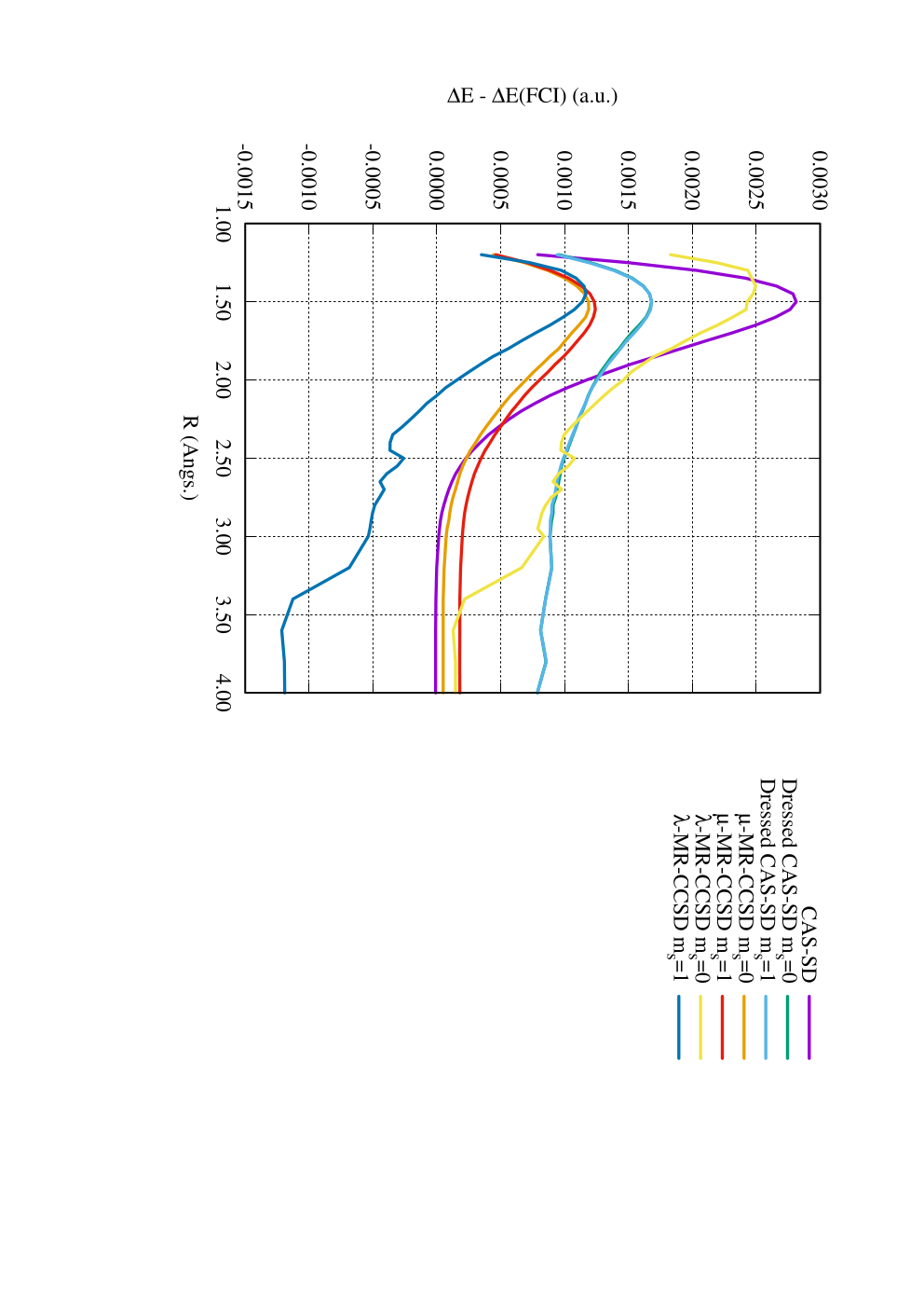
We report here calculations on the triplet state of F2. The reference wave function was prepared in two different ways, both using restricted open-shell Hartree-Fock molecular orbitals. The first reference wave function labeled is a single open-shell determinant, and the second wave function is the triplet , made of two determinants .
To ensure that the CAS-SD is a strict eigenfunction of the operator, we have included in all the determinants with the same space part as the Singles and Doubles with respect to the CAS. These determinants are treated in the same way as Singles and Doubles and are treated variationally in the diagonalizations. Of course, those which are Triples or Quadruples with respect to are excluded from the set of the and have no effect in the dressing.
To reduce the computational cost, the Triples and Quadruples were not augmented with all the determinants with the same space part. The absence of some determinants gives rise to a slight deviation ( a.u.) of from the desired eigenvalue, and it is expected to have some impact on the iterative dressing. It is worth checking the effect of this deviation from the exact spin multiplicity. The first test concerns the comparison of the and components of a triplet state.
In all the cases, the NPE of the CAS-SD (2.6 m) is improved to a value of 1.1–1.5 m. As expected the two variants of the MR-CCSD are strictly equivalent for . Indeed, for both variants the usual single-reference amplitudes are recovered. The amplitudes of the -MR-CCSD lower the curve by 1 m when going from to . The dressed CAS-SD also gives a lower energy, but only by 0.5 m. This is due to the increased number of degrees of freedom in the fit of the amplitudes as no additional constraint is imposed to enforce the -invariance. But when the reference-dependence is introduced via the , it is imposed to recover the CAS-SD wave function which is -invariant, and this step compensates the additional freedom gained in the fitting, and the and MR-CCSD curves differ by less than 0.1 m.
If one considers the error on the singlet-triplet gap with respect to the Full-CI reference, it appears clearly that the -MR-CCSD gives the most accurate results, with errors lying between 0.1 m and 1.3 m along the curve.
Avoided crossing in HF and LiF


We have calculated the potential energy surfaces of the two lowest states of HF, using as reference wave function the CAS(2,2) with state-averaged CAS-SCF molecular orbitals in the aug-cc-pVDZ basis set. Figure 3 shows the NPEs of the ground and excited states. In the ground state, the NPE is 1.8 m for both MR-CCSD variants, but the -MR-CCSD shows some numerical instabilities, as opposed to the -MR-CCSD which gives a very smooth curve.
In the excited state, the situation is different : surprisingly the best NPE is obtained by the CAS-SD, but this may be due to the fact the molecule is particularly favorable to the CAS-SD : both H and H+ have no correlation energy, so the wave functions of the dissociated molecule can be expressed as a product. The two variants of the MR-CCSD agree at short and long distances, but they differ significantly between 2 and 3.0 Å, after the region of the avoided crossing. To understand these differences, we have plotted the two eigenvalues of the two state-specific Hamiltonians, one dressed for the ground state and one dressed for the excited state. It appears that between 2 and 3.0 Å, the lowest eigenvalue of the Hamiltonian dressed for the excited state is very badly described. The reason is that the fitting procedure for the amplitudes is a least-squares fit on the CAS-SD wave function of the state of interest, so the quality of the dressing for the determinants which have small coefficients on the state of interest but large coefficients on the other state will be very low. The -MR-CCSD has amplitudes which depend less on the wave function, so the quality is equivalent on both states, and the choice of these amplitudes is better suited for calculating excited states within the same symmetry.

In figure 5 we have represented the avoided crossing of LiF, also calculated with the aug-cc-pVDZ basis set. The physical situation is similar to HF, but the energy difference between the ground and the excited states is much smaller. A striking result is that the -MR-CCSD, although being state-specific, is able to reproduce very well the whole potential energy surfaces of both states. The position of the avoided crossing is very well reproduced by the three methods : the CAS-SD crosses at 6.3 Å, the Full-CI crosses at 6.8 Åand the dressed CAS-SD and the two MR-CCSD variants cross at 6.9 Å. The -MR-CCSD and -MR-CCSD coincide in the short-range () and in the long range (), but when the two states become very close in energy in the region of the crossing the dressed CAS-SD and the -MR-CCSD are unable to give sensible values. This disappointing result motivates a future work on a multi-state -MR-CCSD.
Sensitivity to the choice Molecular Orbitals


The -MR-CCSD algorithm we propose is in the Jeziorski-Monkhorst framework, so it is not invariant with respect to the choice of molecular orbitals. In this section, we checked its sensitivity to the choice of the MO set by comparing results obtained with pseudo-canonical CAS-SCF orbitals and with localized MOs in the F2 and N2 molecules (figure 6).
In the F2 molecule, using localized MOs is a better choice than the pseudo-canonical MOs. The best NPE is obtained by the -MR-CCSD method with a value of 1.1 m. In the case of N2, the situation is different : the NPE of the -MR-CCSD goes from 0.9 m to 3.7 m, and the NPE of the -MR-CCSD increases from 0.7 m to 1.1 m. On the other hand, the dressed CAS-SD gives a better NPE with local orbitals, going from 1.7 m to 1.1 m.
The fact that the -MR-CCSD is less sensitive to the MO set than the -MR-CCSD can be understood. By changing the MO set, a single excitation rotates into a combination of single and double excitations. In the -MR-CCSD method, the amplitudes are calculated by taking into account the matrix elements of the Hamiltonian, which are of different nature depending on the degree of excitation, so the amplitudes are expected to change significantly. In the -MR-CCSD variant, the amplitudes are adjusted in such a way that they fit the CAS-SD wave function, which is invariant by rotation of the MOs. Therefore, it is expected to be more robust with respect to the MO set.
IV Conclusions
We have proposed a method to determine reference-independent amplitudes by fitting the CAS-SD CI vector. These amplitudes may be used to perform a state-specific iterative dressing of the CAS-SD Hamiltonian in order to take into account the effect of the Triples and Quadruples in the spirit of the Coupled Cluster formalism. Alternatively, these amplitudes may be rescaled to reproduce the exact coefficients of the singles and doubles to introduce a reference-dependent character. In that case, the CAS-SD CI vector is recovered by the application of on the reference wave function, so we reach here the Jeziorski-Monkhorst Coupled Cluster formalism.
The CAS-SD dressed with reference-independent amplitudes gives excellent results for single-bond breaking (F2 and ethane) and the simultaneous breaking of the two O—H bonds of water, with a non-parallelism error lower than the milli-Hartree. When the active space becomes larger, it is necessary to go to the reference-dependent MR-CCSD introducing the factors in Eq. 28. In the case of ethylene and N2, this keeps the NPE to a value close to the milli-Hartree.
We have shown numerically that the here-proposed amplitudes are not very sensitive to the value of for open-shell systems, and to the choice of the molecular orbitals. This is clearly an improvement compared the amplitudes proposed earlier[15]. But we have also shown that the former amplitudes are a better choice when computing excited states of the same symmetry because the here-proposed amplitudes have a much more pronounced state-specific character which may be disadvantageous if the states are too close in energy. This problem can be cured by leaving the state-specific formalism for a multi-state formalism[37], and this will be the object of a future work.
Acknowledgments. This work has been made through generous computational support from CALMIP (Toulouse) under the allocation 2015-0510, and GENCI under the allocation x2015081738.
References
- [1] F. Coester, Nucl. Phys. 7, 421 (1958).
- [2] F. Coester and H. Kümmel, Nucl. Phys. 17, 477 (1960).
- [3] J. Čiźěk, J. Chem. Phys. 45, 4256 (1966).
- [4] R. J. Bartlett, J. Watts, S. Kucharski, and J. Noga, Chem. Phys. Lett. 165, 513 (1990).
- [5] J. Goldstone, Proc. Roy. Soc. A 239, 267 (1957).
- [6] I. Nebot-Gil, J. Sańchez-Mariń, J. P. Malrieu, J. L. Heully, and D. Maynau, J. Chem. Phys. 103, 2576 (1995).
- [7] J. P. Malrieu, P. Durand, and J. P. Daudey, J. Phys. A : Math. Gen. 18, 809 (1985).
- [8] B. Kirtman, J. Chem. Phys. 75, 798 (1981).
- [9] D. I. Lyakh, M. Musiał, V. F. Lotrich, and R. J. Bartlett, Chem. Rev. 112, 182 (2012).
- [10] U. S. Mahapatra, B. Datta, and D. Mukherjee, Mol. Phys. 94, 157 (1998).
- [11] S. Das, D. Mukherjee, and M. Kállay, J. Chem. Phys. 132, 074103 (2010).
- [12] A. Szabados, J. Chem. Phys. 134, 174113 (2011).
- [13] U. S. Mahapatra, B. Datta, and D. Mukherjee, J. Chem. Phys. 110, 6171 (1999).
- [14] J. Meller, J. P. Malrieu, and R. Caballol, J. Chem. Phys. 104, 4068 (1996).
- [15] E. Giner, G. David, A. Scemama, and J. P. Malrieu, J. Chem. Phys. 144, 064101 (2016).
- [16] B. Jeziorski and H. J. Monkhorst, Phys. Rev. A 24, 1668 (1981).
- [17] F. A. Evangelista and J. Gauss, J. Chem. Phys. 134, 114102 (2011).
- [18] M. Hanauer and A. Köhn, J. Chem. Phys. 136, 204107 (2012).
- [19] L. F. Richardson, Phil. Trans. Roy. Soc. A 210, 307 (1911).
- [20] G. Golub and W. Kahan, J. SIAM Ser. B 2, 205 (1965).
- [21] A. Engels-Putzka and M. Hanrath, J. of Mol. Struc.: THEOCHEM 902, 59 (2009).
- [22] G. D. Purvis and R. J. Bartlett, J. Chem. Phys. 76, 1910 (1982).
- [23] G. D. Purvis, R. Shepard, F. B. Brown, and R. J. Bartlett, Int. J. Quantum Chem. 23, 835 (1983).
- [24] W. D. Laidig and R. J. Bartlett, Chem. Phys. Lett. 104, 424 (1984).
- [25] M. Kállay, P. G. Szalay, and P. R. Surján, J. Chem. Phys. 117, 980 (2002).
- [26] M. Hanrath, J. Chem. Phys. 123, 084102 (2005).
- [27] F. A. Evangelista, W. D. Allen, and H. F. Schaefer, J. Chem. Phys. 125, 154113 (2006).
- [28] F. A. Evangelista, E. Prochnow, J. Gauss, and H. F. Schaefer, J. Chem. Phys. 132, 074107 (2010).
- [29] M. Hanauer and A. Köhn, J. Chem. Phys. 134, 204111 (2011).
- [30] Y. A. Aoto and A. Köhn, J. Chem. Phys. 144, 074103 (2016).
- [31] T. H. Dunning, J. Chem. Phys. 90, 1007 (1989).
- [32] M. W. Schmidt, K. K. Baldridge, J. A. Boatz, S. T. Elbert, M. S. Gordon, J. H. Jensen, S. Koseki, N. Matsunaga, K. A. Nguyen, S. Su, T. L. Windus, M. Dupuis, and J. A. Montgomery, J. of Comput. Chem. 14, 1347 (1993).
- [33] A. Scemama, T. Applencourt, Y. Garniron, E. Giner, G. David, and M. Caffarel, “Quantum package v1.0,” (2016), https://github.com/LCPQ/quantum_package.
- [34] B. Huron, P. Rancurel, and J. Malrieu, J. Chem. Phys. 58, 5745 (1973).
- [35] S. Evangelisti, J. Daudey, and J. Malrieu, Chem. Phys. 75, 91 (1983).
- [36] E. Giner, A. Scemama, and M. Caffarel, Can. J. Chem. 91, 879 (2013).
- [37] J.-P. Malrieu, Mol. Phys. 111, 2451 (2013).