跳到论文正文
W Papers独立论文阅读器 arXiv:1701.04643 论文正文 计算阅读时间 · 0%
引用这篇论文根据当前论文元数据生成,正式投稿前建议核对。


License: arXiv.org perpetual non-exclusive license
arXiv:1701.04643v1 [cond-mat.mtrl-sci] 17 Jan 2017

Discretization error cancellation in electronic structure calculation:
a quantitative study

Eric Cancès Note: cances@cermics.enpc.fr Affiliation: CERMICS, Ecole des Ponts and INRIA Paris, 6 & 8 Avenue Blaise Pascal, 77455 Marne-la-Vallée, France    Geneviève Dusson Note: dusson@ljll.math.upmc.fr Affiliation: Sorbonne Universités, UPMC Univ. Paris 06 and CNRS, UMR 7598, Laboratoire Jacques-Louis Lions, F-75005, Paris, France, and Sorbonne Universités, UPMC Univ. Paris 06, Institut du Calcul et de la Simulation, F-75005, Paris, France
August 24, 2026
Abstract

It is often claimed that error cancellation plays an essential role in quantum chemistry and first-principle simulation for condensed matter physics and materials science. Indeed, while the energy of a large, or even medium-size, molecular system cannot be estimated numerically within chemical accuracy (typically 1 kcal/mol or 1 mHa), it is considered that the energy difference between two configurations of the same system can be computed in practice within the desired accuracy.

The purpose of this paper is to provide a quantitative study of discretization error cancellation. The latter is the error component due to the fact that the model used in the calculation (e.g. Kohn-Sham LDA) must be discretized in a finite basis set to be solved by a computer. We first report comprehensive numerical simulations performed with Abinit [1, 2] on two simple chemical systems, the hydrogen molecule on the one hand, and a system consisting of two oxygen atoms and four hydrogen atoms on the other hand. We observe that errors on energy differences are indeed significantly smaller than errors on energies, but that these two quantities asymptotically converge at the same rate when the energy cut-off goes to infinity. We then analyze a simple one-dimensional periodic Schrödinger equation with Dirac potentials, for which analytic solutions are available. This allows us to explain the discretization error cancellation phenomenon on this test case with quantitative mathematical arguments.

I Introduction

Error control is a central issue in molecular simulation. The error between the computed value of a given physical observable (e.g. the dissociation energy of a molecule) and the exact one, has several origins. First, there is always a discrepancy between the physical reality and the reference model, here the NN-body Schrödinger equation, possibly supplemented with Breit terms to account for relativistic effects. However, at least for the atoms of the first three rows of the periodic table, this reference model is in excellent agreement with experimental data, and can be considered as exact in most situations of interest. The overall error is therefore the sum of the following components:

  1. 1.

    the model error, that is the difference between the value of the observable for the reference model, which is too complicated to solve in most cases, and the value obtained with the chosen approximate model (e.g. the Kohn-Sham LDA model), assuming that the latter can be solved exactly;

  2. 2.

    the discretization error, that is the difference between the value of the observable for the approximate model and the value obtained with the chosen discretization of the approximate model. Indeed, the approximate model is typically an infinite dimensional minimization problem, or a system of partial differential equations, which must be discretized to be solvable by a computer, using e.g. a Gaussian atomic basis set, or a planewave basis;

  3. 3.

    the algorithmic error, which is the difference between the value of the observable obtained with the exact solution of the discretized approximate model, and the value computed with the chosen algorithm. The discretized approximate models are indeed never solved exactly; they are solved numerically by iterative algorithms (e.g. SCF algorithms, Newton methods), which, in the best case scenario, only converge in the limit of an infinite number of iterations. In practice, stopping criteria are used to exit the iteration loop when the error at iteration kk, measured in terms of differences between two consecutive iterates or, better, by some norm of some residual, is below a prescribed threshold. If the stopping criterion is very tight, the algorithmic error can become very small, … or not! For instance, if the discretized approximate model is a non convex optimization problem, there is no guarantee that the numerical algorithm will converge to a global minimum. It may converge to a local, non-global minimum, leading to a non-zero algorithmic error even in the limit of an infinitely tight stopping criterion;

  4. 4.

    the implementation error, which may, obviously, be due to bugs, but does not vanish in the absence of bugs, because of round-off errors: in molecular simulation packages, most operations are implemented in double precision, and the resulting round-off errors can accumulate, especially for very large systems;

  5. 5.

    the computing error, due to random hardware failures (miswritten or misread bits). This component of the error is usually negligible in today’s standard computations, but is expected to become critical in future exascale architectures [3].

Quantifying these different sources of errors is an interesting purpose for two reasons. First, guaranteed estimates on these five components of the error would allow one to supplement the computed value of the observable returned by the numerical simulation with guaranteed error bars (certification of the result). Second, they would allow one to choose the parameters of the simulation (approximate model, discretization parameters, algorithm and stopping criteria, data structures, etc.) in an optimal way in order to minimize the computational effort required to reach the target accuracy.

The construction of guaranteed error estimators for electronic structure calculation is a very challenging task. Some progress has however been made in the last few years, regarding notably the discretization and algorithmic errors for Kohn-Sham LDA calculations. A priori discretization error estimates have been constructed in [4] for planewave basis sets, and then in [5] for more general variational discretization methods. A posteriori error estimators of the discretization error have been proposed in [6, 7, 8]. A combined study of both the discretization and algorithmic errors was published in [9] (see also [10]). We also refer to [11, 12, 13, 14, 15, 16, 17, 18, 19, 20] and references therein for other works on error analysis for electronic structure calculation.

In all the previous works on this topic we are aware of, the purpose was to estimate, for a given nuclear configuration RR of the system, the difference between the ground state energy ERE_{R} (or another observable) obtained with the continuous approximate model under consideration (e.g. Kohn-Sham LDA) and its discretized counterpart denoted by ER,NE_{R,N}, where NN is the discretization parameter. The latter is typically the number of basis functions in the basis set for local combination of atomic orbitals (LCAO) methods [21], the inverse fineness of the grid or the mesh for finite difference (FD) and finite element (FE) methods [22, 23, 24, 25], the cut-off parameter in energy or momentum space for planewave (PW) discretization methods [1, 26, 27], or the inverse grid spacing and the coarse and fine region multipliers for wavelet (WL) methods [28]. In variational approximation methods (LCAO, FE, PW, and WL), the discretization error ER,N−ERE_{R,N}-E_{R} is always nonnegative by construction. In systematically improvable methods (FD, FE, PW, and WL), this quantity goes to zero when NN goes to infinity with a well-understood rate of convergence depending on the smoothness of the pseudopotential (see [4] for the PW case). However, in most applications, the discretization parameters are not tight enough for the discretization error to be lower than the target accuracy, which is typically of the order of 1 kcal/mol or 1 mHa (recall that 1 mHa ≃\simeq 0.6275 kcal/mol ≃\simeq 27.2 meV, which corresponds to an equivalent temperature of about 316 K). It is often advocated that this is not an issue since the real quantity of interest is not the value of the energy ERE_{R} for a particular nuclear configuration RR, but the energy difference ER1−ER2E_{R_{1}}-E_{R_{2}} between two different configurations R1R_{1} and R2R_{2}. It is indeed expected that

|(ER1,N−ER2,N)−(ER1−ER2)|≪|ER1,N−ER1|+|ER2,N−ER2|,|(E_{R_{1},N}-E_{R_{2},N})-(E_{R_{1}}-E_{R_{2}})|\ll|E_{R_{1},N}-E_{R_{1}}|+|E_{R_{2},N}-E_{R_{2}}|,

that is, the numerical error on the energy difference between the two configurations is much smaller than the sum of the discretization errors on the energies of each configuration. This expected phenomenon goes by the name of (discretization) error cancellation in the Physics and Chemistry literatures.

Obviously, for variational discretization methods, ERj,N−ERj≥0E_{R_{j},N}-E_{R_{j}}\geq 0 so that both discretization errors have the same sign, leading to

|(ER1,N−ER2,N)−(ER1−ER2)|\displaystyle|(E_{R_{1},N}-E_{R_{2},N})-(E_{R_{1}}-E_{R_{2}})| =|(ER1,N−ER1)−(ER2,N−ER2)|\displaystyle=\left|(E_{R_{1},N}-E_{R_{1}})-(E_{R_{2},N}-E_{R_{2}})\right|
≤max⁡(ER1,N−ER1,ER2,N−ER2),\displaystyle\leq\max\left(E_{R_{1},N}-E_{R_{1}},E_{R_{2},N}-E_{R_{2}}\right),

but this does not explain the magnitude of the error cancellation phenomenon. The commonly admitted qualitative argument usually raised to explain this phenomenon is that the errors ER1,N−ER1E_{R_{1},N}-E_{R_{1}} and ER2,N−ER2E_{R_{2},N}-E_{R_{2}} are of the same nature and almost annihilate one another.

The purpose of this article is to provide a quantitive analysis of discretization error cancellation for PW discretization methods. First, we report in Section II two systematic numerical studies on, respectively, the hydrogen molecule and a simple system consisting of six atoms. For these systems, we are able to perform very accurate calculations with high PW cut-offs, which provide excellent approximations of the ground state energy ERE_{R}. We then compute, for two different configurations R1R_{1} and R2R_{2}, the error cancellation factor

0≤QN:=|(ER1,N−ER2,N)−(ER1−ER2)||ER1,N−ER1|+|ER2,N−ER2|≤1.0\leq Q_{N}:=\frac{|(E_{R_{1},N}-E_{R_{2},N})-(E_{R_{1}}-E_{R_{2}})|}{|E_{R_{1},N}-E_{R_{1}}|+|E_{R_{2},N}-E_{R_{2}}|}\leq 1.

We observe that this ratio is indeed small (typically between 10−310^{-3} and 10−110^{-1} depending on the system and on the configurations R1R_{1} and R2R_{2}), and that it does not vary much with NN. In Section III, we introduce a toy model consisting of seeking the ground state of a one-dimensional linear periodic Schrödinger equation with Dirac potentials:

(−d2d​x2−∑m∈ℤz1​δm−∑m∈ℤz2​δm+R)​uR=ER​uR,∫01uR2​(x)​𝑑x=1,\left(-\frac{d^{2}}{dx^{2}}-\sum_{m\in{\mathbb{Z}}}z_{1}\delta_{m}-\sum_{m\in{\mathbb{Z}}}z_{2}\delta_{m+R}\right)u_{R}=E_{R}u_{R},\qquad\int_{0}^{1}u_{R}^{2}(x)dx=1,

for which we can prove that the error cancellation factor QNQ_{N} converges to a fixed number 0<Q∞<10<Q_{\infty}<1 when NN goes to infinity. Interestingly, it is possible to obtain a simple explicit expression of Q∞Q_{\infty}, which only depends on z1z_{1}, z2z_{2} and on uR1​(0)2u_{R_{1}}(0)^{2}, uR2​(0)2u_{R_{2}}(0)^{2}, uR1​(R1)2u_{R_{1}}(R_{1})^{2}, uR1​(R2)2u_{R_{1}}(R_{2})^{2}, i.e. on the values of the densities ρR1=uR12\rho_{R_{1}}=u_{R_{1}}^{2} and ρR1=uR22\rho_{R_{1}}=u_{R_{2}}^{2} at the singularities of the potential.

II Discretization error cancellation in planewave calculations

We present here some numerical simulations on two systems: the H2H_{2} molecule and a system consisting of two oxygen atoms and four hydrogen atoms. The simulations are done in a cubic supercell of size 10×\times10×\times10 bohrs with the Abinit simulation package [1, 2]. The chosen approximate model is the periodic Kohn-Sham LDA model [29] with the parametrization and the pseudopotential proposed in [30]. For each configuration RR, we compute a reference ground state energy ERE_{R} taking a high energy cutoff Ecut=400E_{\rm cut}=400 Ha. We then compute approximate energies for N=EcutN=E_{\rm cut} varying from 5 to 105 Ha by steps of 5 Ha. The so-obtained energies are denoted by ER,NE_{R,N}.

For two given configurations R1R_{1} and R2R_{2} of the same system, we compute SNS_{N}, the sum of the discretization errors on the energies of the two configurations (note that ER,N−ER≥0E_{R,N}-E_{R}\geq 0 since PW is a variational approximation method), and DND_{N}, the discretization error on the energy difference:

SN=(ER1,N−ER1)+(ER2,N−ER2)andDN=|(ER1,N−ER2,N)−(ER1−ER2)|,S_{N}=(E_{R_{1},N}-E_{R_{1}})+(E_{R_{2},N}-E_{R_{2}})\quad\text{and}\quad D_{N}=\left|(E_{R_{1},N}-E_{R_{2},N})-(E_{R_{1}}-E_{R_{2}})\right|,

as well as the error cancellation factor

QN=DNSN=|(ER1,N−ER2,N)−(ER1−ER2)|(ER1,N−ER1)+(ER2,N−ER2).Q_{N}=\frac{D_{N}}{S_{N}}=\frac{\left|(E_{R_{1},N}-E_{R_{2},N})-(E_{R_{1}}-E_{R_{2}})\right|}{(E_{R_{1},N}-E_{R_{1}})+(E_{R_{2},N}-E_{R_{2}})}.

II.1 Ground state potential energy surface of the H2 molecule

In all our calculations, the H2H_{2} molecule lies on the xx axis and is centered at the origin. The parameter RR is here the interatomic distance in bohrs.

We numerically observe that DND_{N} is smaller than SNS_{N} by a factor of 10 to 100, and that the error cancellation factor QNQ_{N} is smaller when the two interatomic distances are close to each other (R1≃R2R_{1}\simeq R_{2}). Morevoer, QNQ_{N} is almost constant with respect to the cut-off energy NN.

In Figure 1, we present detailed results for two different pairs of configurations. On the top, the configurations are rather close since the interatomic distances are R1=1.464R_{1}=1.464 and R2=1.524R_{2}=1.524 bohr. For this approximate model, the equilibrium distance is about Req≃1.464R_{\rm eq}\simeq 1.464 bohrs (the experimental value is Reqexp≃1.401R_{\rm eq}^{\rm exp}\simeq 1.401 bohrs). The energy difference is better approximated by a factor of about 50 compared to the energies (QN≃0.02Q_{N}\simeq 0.02). Moreover the log-log plots of SNS_{N} and DND_{N} are almost parallel, which suggests that there is no improvement in the order of convergence when considering energy differences instead of energies; only the prefactor is improved. This is confirmed by the plots of the error cancellation factor QNQ_{N}, showing that this ratio does not vary much with NN. On the bottom, the configurations are further apart. The interatomic distances are R1=1.344R_{1}=1.344 and R2=1.704R_{2}=1.704 bohrs. We observe a similar behavior except that the error cancellation phenomenon is less pronounced (QN≃0.1Q_{N}\simeq 0.1).

Figure 1: Convergence plots of the quantities SNS_{N} and DND_{N} (left) and of the error cancellation factor QN=DN/SNQ_{N}=D_{N}/S_{N} (right) for two different pairs of interatomic distances for the H2H_{2} molecule. Top: R1=1.464R_{1}=1.464 and R2=1.524R_{2}=1.524 bohrs. Bottom: R1=1.344R_{1}=1.344 and R2=1.704R_{2}=1.704 bohrs.

We then compare in Table 1 the values of SNS_{N} and DND_{N} for different pairs of configurations and for two values of N=EcutN=E_{\rm cut}: a rather coarse energy cut-off N=30N=30 Ha, and a quite fine one N=100N=100 Ha. One configuration is kept fixed (R1=1.284R_{1}=1.284 bohrs), while the second one varies from R2=1.344R_{2}=1.344 bohrs (close configurations) to R2=1.764R_{2}=1.764 bohrs (distant configurations). We also report, for each pair of configurations, the minimum, maximum, and mean values of QNQ_{N} over the different tested energy cutoffs 5≤N≤1055\leq N\leq 105 Ha. We also observe that QNQ_{N} increases with R2−R1R_{2}-R_{1} on the range R2=[1.344,1.764]R_{2}=[1.344,1.764].

R1R_{1} R2R_{2} SN=30S_{N=30} DN=30D_{N=30} SN=100S_{N=100} DM=100D_{M=100} min⁡(QN)\min(Q_{N}) max⁡(QN)\max(Q_{N}) mean​(QN)\text{mean}(Q_{N})
1.284 1.344 9.410 0.1985 0.09157 0.00112 0.0103 0.0340 0.0212
1.284 1.404 9.268 0.3408 0.08990 0.00279 0.0216 0.0633 0.0413
1.284 1.464 9.160 0.4491 0.08772 0.00497 0.0375 0.0895 0.0610
1.284 1.524 9.065 0.5436 0.08552 0.00717 0.0544 0.1107 0.0802
1.284 1.584 8.969 0.6394 0.08380 0.00889 0.0713 0.1285 0.0985
1.284 1.644 8.863 0.7456 0.08274 0.00995 0.0841 0.1455 0.1151
1.284 1.704 8.744 0.8646 0.08213 0.01056 0.0983 0.1642 0.1302
1.284 1.764 8.615 0.9937 0.08154 0.01115 0.1072 0.1802 0.1440
Table 1: Comparison of SNS_{N}, DND_{N} and QNQ_{N} for different atomic configurations of the H2 molecule. Distances are in bohrs, energies in mHa.

II.2 Energy of a simple chemical reaction

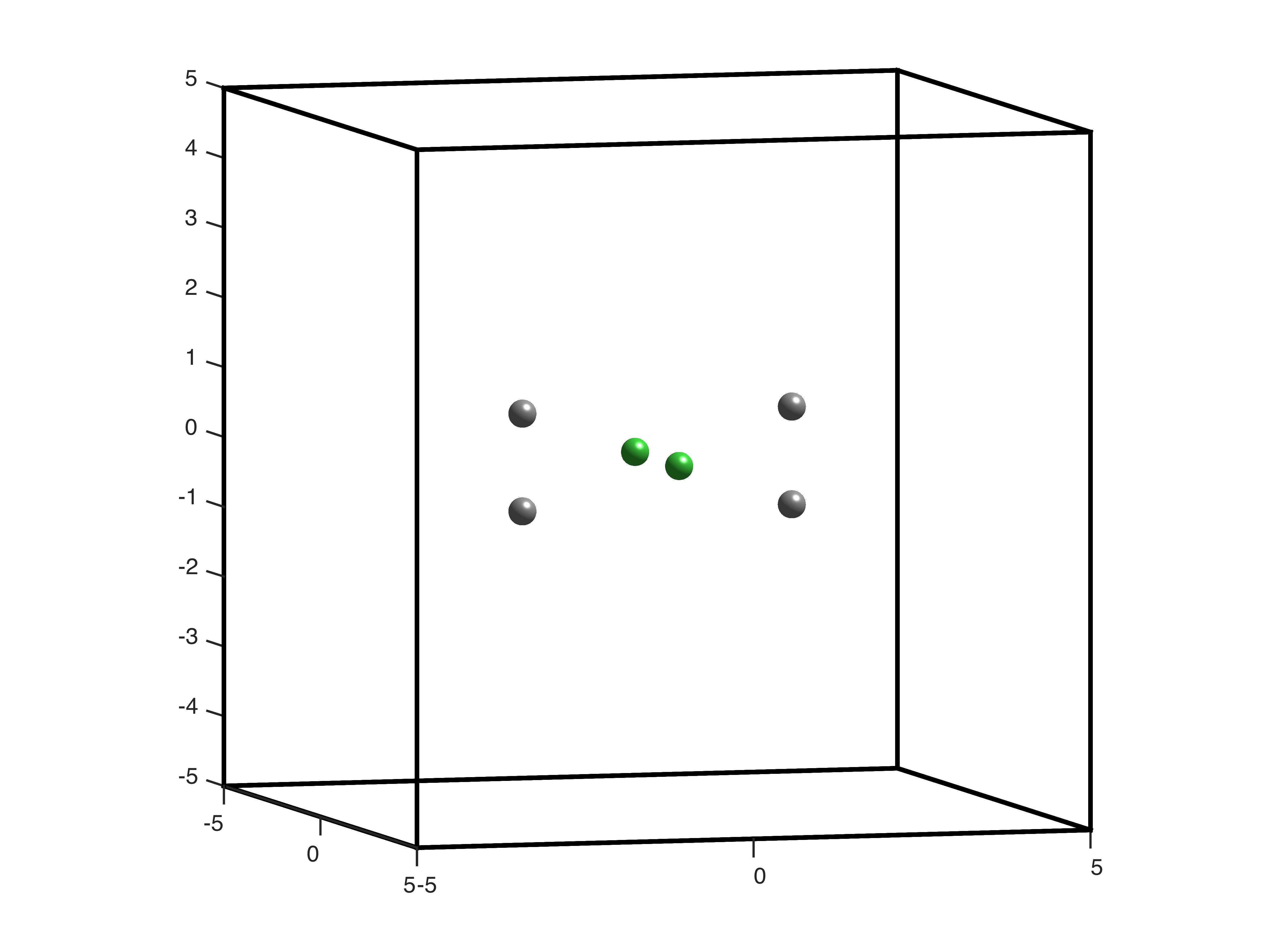
In this section, we consider the energy difference between two very different configurations of a system consisting of two oxygen atoms and four hydrogen atoms. The first configuration, denoted by R1R_{1}, corresponds to the chemical system 2 H2O (two water molecules) and the second one, denoted by R2R_{2}, to the chemical system 2 H2 + O2, all these molecules being in their equilibrium geometry (see Figure 2). The energy difference between the two configurations thus provides a rough estimate of the energy of the chemical reaction
2 H2 + O2⟶2 H2O.\mbox{2 H${}_{2}$ + O${}_{2}$}\;\longrightarrow\;\mbox{2 H${}_{2}$O}.
Refer to caption Refer to caption
Figure 2: Graphical representation of the two atomic configurations whose energies are compared. Oxygen atoms are in green, hydrogen atoms in black.

We can observe on Figure 3 and Table 2 a similar behavior as for H2, but with a better error cancellation factor (QN≃0.005Q_{N}\simeq 0.005).

Figure 3: Convergence plots of the quantities SNS_{N} and DND_{N} (left) and of the error cancellation factor QN=DN/SNQ_{N}=D_{N}/S_{N} (right) for the two different configurations displayed on Figure 2.
SN=30S_{N=30} DN=30D_{N=30} SN=100S_{N=100} DN=100D_{N=100} min⁡(QN)\min(Q_{N}) max⁡(QN)\max(Q_{N}) mean​(QN)\text{mean}(Q_{N})
1403 5.726 15.12 0.0485 0.0005036 0.008986 0.004640
Table 2: Comparison of SNS_{N}, DND_{N} (in mHa) and QNQ_{N} for the two different configurations displayed on Figure 2.

III Mathematical analysis of a toy model

We now present a simple one-dimensional periodic linear Schrödinger model for which the discretization error cancellation phenomenon observed in the previous section can be explained with full mathematical rigor.

We denote by

Lper2:={u∈Lloc2​(ℝ)|u​is​ 1−periodic}L^{2}_{\rm per}:=\left\{u\in L^{2}_{\rm loc}({\mathbb{R}})\;\middle|\;u\;\text{is}\;1-\text{periodic}\right\}

the vector space of the 1-periodic locally square integrable real-valued functions on ℝ{\mathbb{R}}, and by

Hper1:={u∈Lper2|u′∈Lper2}H^{1}_{\rm per}:=\left\{u\in L^{2}_{\rm per}\;\middle|\;u^{\prime}\in L^{2}_{\rm per}\right\}

the associated order-1 Sobolev space. For two given parameters z1,z2>0z_{1},z_{2}>0, we consider the family of problems, indexed by R∈(0,1)R\in(0,1), consisting in finding the ground state (uR,ER)∈Hper1×ℝ(u_{R},E_{R})\in H^{1}_{\rm per}\times\mathbb{R} of

{(−d2d​x2−∑m∈ℤz1​δm−∑m∈ℤz2​δm+R)​uR=ER​uR,∫01uR2(x)dx=1,uR≥0,\left\{\begin{array}[]{l}\displaystyle\left(-\frac{d^{2}}{dx^{2}}-\sum_{m\in{\mathbb{Z}}}z_{1}\delta_{m}-\sum_{m\in{\mathbb{Z}}}z_{2}\delta_{m+R}\right)u_{R}=E_{R}u_{R},\\ \displaystyle\int_{0}^{1}u_{R}^{2}(x)dx=1,\quad u_{R}\geq 0,\\ \end{array}\right. (1)

where δa\delta_{a} denotes the Dirac mass at point a∈ℝa\in{\mathbb{R}}. A variational formulation of the problem is: find the ground state (uR,ER)∈Hper1×ℝ(u_{R},E_{R})\in H^{1}_{\rm per}\times\mathbb{R} of

{∀v∈H1per,∫01u′R(x)v′(x)dx−z1uR(0)v(0)−z2uR(R)v(R)=ER∫01uR(x)v(x)dx,∫01uR2(x)dx=1,uR≥0.\left\{\begin{array}[]{l}\displaystyle\forall v\in H^{1}_{\rm per},\;\int_{0}^{1}u^{\prime}_{R}(x)v^{\prime}(x)dx-z_{1}u_{R}(0)v(0)-z_{2}u_{R}(R)v(R)=E_{R}\int_{0}^{1}u_{R}(x)v(x)dx,\\ \displaystyle\int_{0}^{1}u_{R}^{2}(x)dx=1,\quad u_{R}\geq 0.\\ \end{array}\right. (2)
Remark 1.

The ground state eigenvalue ERE_{R} is negative. Indeed, using the variational characterization of the ground state energy, we get

ER=minv∈Hper1∖{0}⁡∫01v′​(x)2​𝑑x−z1​v​(0)2−z2​v​(R)2∫01v2​(x)​𝑑x<0,\displaystyle E_{R}=\min_{\displaystyle v\in H^{1}_{\rm per}\setminus\left\{0\right\}}\frac{\displaystyle\int_{0}^{1}v^{\prime}(x)^{2}dx-z_{1}v(0)^{2}-z_{2}v(R)^{2}}{\displaystyle\int_{0}^{1}v^{2}(x)dx}<0,

since the Rayleigh quotient is equal to −z1−z2<0-z_{1}-z_{2}<0 for the constant test function v=1v=1.

Denoting by kR=−ERk_{R}=\sqrt{-E_{R}}, we have

{uR​(x)=A​ekR​x+B​e−kR​x,∀x∈[0,R],uR​(x)=C​ekR​x+D​e−kR​x,∀x∈[R−1,0),\left\{\begin{array}[]{ll}u_{R}(x)=Ae^{k_{R}x}+Be^{-k_{R}x},&\quad\forall x\in[0,R],\\ u_{R}(x)=Ce^{k_{R}x}+De^{-k_{R}x},&\quad\forall x\in[R-1,0),\end{array}\right. (3)

where AA, BB, CC, and DD are real-valued constants. Since the function uRu_{R} is 1-periodic and continuous on ℝ{\mathbb{R}} and its derivative satisfies the jump conditions uR′​(m+0)−uR′​(m−0)=−z1​uR​(m)u_{R}^{\prime}(m+0)-u_{R}^{\prime}(m-0)=-z_{1}u_{R}(m) and uR′​(m+R+0)−uR′​(m+R−0)=−z2​uR​(m+R)u_{R}^{\prime}(m+R+0)-u_{R}^{\prime}(m+R-0)=-z_{2}u_{R}(m+R) for all m∈ℤm\in{\mathbb{Z}}, the coefficients AA, BB, CC, DD solve the linear system

(11−1−1ekR​Re−kR​R−ekR​(R−1)−e−kR​(R−1)kR+z1−kR+z1−kRkR(kR−z2)​ekR​R−(kR+z2)​e−kR​R−kR​ekR​(R−1)kR​e−kR​(R−1))⏟M⁡(kR)​(ABCD)=(0000).\underbrace{\left(\begin{array}[]{cccc}1&1&-1&-1\\ e^{k_{R}R}&e^{-k_{R}R}&-e^{k_{R}(R-1)}&-e^{-k_{R}(R-1)}\\ k_{R}+z_{1}&-k_{R}+z_{1}&-k_{R}&k_{R}\\ (k_{R}-z_{2})e^{k_{R}R}&-(k_{R}+z_{2})e^{-k_{R}R}&-k_{R}e^{k_{R}(R-1)}&k_{R}e^{-k_{R}(R-1)}\end{array}\right)}_{M(k_{R})}\left(\begin{array}[]{c}A\\ B\\ C\\ D\end{array}\right)=\left(\begin{array}[]{c}0\\ 0\\ 0\\ 0\end{array}\right).

The wave vector kRk_{R} is the lowest positive root of the function k↦det⁡(M⁡(k))k\mapsto{\rm det}(M(k)). The coefficients (A,B,C,D)(A,B,C,D) are then uniquely determined by the normalization condition ‖uR‖Lper2=1\|u_{R}\|_{L^{2}_{\rm per}}=1 and the positivity of uRu_{R}. Exact solutions for two different values of the triplet of parameters (z1,z2,R)(z_{1},z_{2},R) are plotted in Figure 4.

Figure 4: Plot of the exact solutions of (1) for two sets of parameters.

An approximate solution of the problem is obtained using the PW discretization method. Denoting by

XN:=Span{vN(x)=∑k∈ℤ,|k|≤Nv^ke2​π​i​k​x|v^k∈ℂ,v^−k=v^k¯}⊂Hper1,X_{N}:=\text{Span}\left\{v_{N}(x)=\sum_{k\in{\mathbb{Z}},\;|k|\leq N}\widehat{v}_{k}e^{2\pi ikx}\;\bigg|\;\widehat{v}_{k}\in{\mathbb{C}},\;\widehat{v}_{-k}=\overline{\widehat{v}_{k}}\right\}\subset H^{1}_{\rm per},

the variational approximation of problem (2) in XNX_{N} consists in computing the ground state (uR,N,ER,N)∈XN×ℝ(u_{R,N},E_{R,N})\in X_{N}\times{\mathbb{R}} of

{∀vN∈XN,∫01uR,N′vN′−z1uR,N(0)vN(0)−z2uR,N(R)vN(R)=ER,N∫01uR,NvN,∫01uR,N2=1,∫01uR,N≥0.\left\{\begin{array}[]{l}\displaystyle\forall v_{N}\in X_{N},\quad\int_{0}^{1}u_{R,N}^{\prime}v_{N}^{\prime}-z_{1}u_{R,N}(0)v_{N}(0)-z_{2}u_{R,N}(R)v_{N}(R)\ =E_{R,N}\int_{0}^{1}u_{R,N}v_{N},\\ \displaystyle\int_{0}^{1}u_{R,N}^{2}=1,\quad\int_{0}^{1}u_{R,N}\geq 0.\\ \end{array}\right. (4)

The conditions v^−k=v^k¯\widehat{v}_{-k}=\overline{\widehat{v}_{k}} in the definition of XNX_{N} is equivalent to imposing that the elements of XNX_{N} are real-valued functions. For convenience, the discretization parameter NN here corresponds to the cut-off in momentum space. As above, we consider the error cancellation factor

QN=|(ER1,N−ER2,N)−(ER1−ER2)|(ER1,N−ER1)+(ER2,N−ER2)\displaystyle Q_{N}=\frac{|(E_{R_{1},N}-E_{R_{2},N})-(E_{R_{1}}-E_{R_{2}})|}{(E_{R_{1},N}-E_{R_{1}})+(E_{R_{2},N}-E_{R_{2}})} (5)

associated with the pair of configurations (R1,R2)(R_{1},R_{2}).

Note that imposing the condition ∫01uR,N≥0\int_{0}^{1}u_{R,N}\geq 0, we ensure that the discrete eigenfunction uR,Nu_{R,N} will approximate the positive eigenfunction uRu_{R} to the continuous problem (1) and not −uR-u_{R}.

Theorem 1 (Asymptotic expressions of the energy error and of the error cancellation factor).

For all z1,z2>0z_{1},z_{2}>0 and R∈(0,1)R\in(0,1), we have for all ϵ>0\epsilon>0,

ER,N−ER=αRN−αR2​N2+βR,N(1)N+γRN​ηR,N+o⁡(1N3−ϵ),E_{R,N}-E_{R}=\frac{\alpha_{R}}{N}-\frac{\alpha_{R}}{2N^{2}}+\frac{\beta^{(1)}_{R,N}}{N}+\frac{\gamma_{R}}{N}\eta_{R,N}+o\left(\frac{1}{N^{3-\epsilon}}\right), (6)

where

αR:=z12​uR​(0)2+z22​uR​(R)22​π2,γR:=z1​z2​uR​(0)​uR​(R)π2,ηR,N:=N​∑k=N+1+∞cos⁡(2​π​k​R)k2,\alpha_{R}:=\frac{z_{1}^{2}u_{R}(0)^{2}+z_{2}^{2}u_{R}(R)^{2}}{2\pi^{2}},\quad\gamma_{R}:=\frac{z_{1}z_{2}u_{R}(0)u_{R}(R)}{\pi^{2}},\quad\eta_{R,N}:=N\sum_{k=N+1}^{+\infty}\frac{\cos(2\pi kR)}{k^{2}},
βR,N(1):=z12​uR​(0)​(uR,N​(0)−uR​(0))+z22​uR​(R)​(uR,N​(R)−uR​(R))2​π2.\beta^{(1)}_{R,N}:=\frac{z_{1}^{2}u_{R}(0)(u_{R,N}(0)-u_{R}(0))+z_{2}^{2}u_{R}(R)(u_{R,N}(R)-u_{R}(R))}{2\pi^{2}}.

In addition

|ηR,N|≤min⁡(1,2+π38|sin⁡(π​R)|​N),|\eta_{R,N}|\leq\min\left(1,\frac{2+\frac{\pi^{3}}{8}}{|\sin(\pi R)|N}\right),

and for all ϵ>0\epsilon>0, there exists Cϵ∈ℝ+C_{\epsilon}\in{\mathbb{R}}_{+} such that

|βR,N(1)|≤CϵN1−ϵ.|\beta^{(1)}_{R,N}|\leq\frac{C_{\epsilon}}{N^{1-\epsilon}}.

As a consequence, we have for all z1,z2>0z_{1},z_{2}>0 and all R1,R2∈(0,1)R_{1},R_{2}\in(0,1),

limN→+∞QN=|αR1−αR2|αR1+αR2=|z12​(uR1​(0)2−uR2​(0)2)+z22​(uR1​(R1)2−uR2​(R2)2)|z12​(uR1​(0)2+uR2​(0)2)+z22​(uR1​(R1)2+uR2​(R2)2).\lim\limits_{N\to+\infty}Q_{N}=\frac{|\alpha_{R_{1}}-\alpha_{R_{2}}|}{\alpha_{R_{1}}+\alpha_{R_{2}}}=\frac{\left|z_{1}^{2}\left(u_{R_{1}}(0)^{2}-u_{R_{2}}(0)^{2}\right)+z_{2}^{2}\left(u_{R_{1}}(R_{1})^{2}-u_{R_{2}}(R_{2})^{2}\right)\right|}{z_{1}^{2}(u_{R_{1}}(0)^{2}+u_{R_{2}}(0)^{2})+z_{2}^{2}(u_{R_{1}}(R_{1})^{2}+u_{R_{2}}(R_{2})^{2})}. (7)

The proof of the above theorem is given in Appendix. We deduce from (6) that the discretization error ER,N−ERE_{R,N}-E_{R} on the energy of the configuration RR is the sum of

  1. 1.

    a leading term αR​N−1\alpha_{R}N^{-1} of order 1 (in N−1N^{-1});

  2. 2.

    three terms −1/2αRN−2-1/2\alpha_{R}N^{-2}, βR,N(1)​N−1\beta^{(1)}_{R,N}N^{-1}, and γR​N−1​ηR,N\gamma_{R}N^{-1}\eta_{R,N} which are roughly of order 2;

  3. 3.

    higher order terms which are roughly of order 33 and above.

The leading term αR​N−1\alpha_{R}N^{-1} has a very simple expression and the prefactor αR\alpha_{R} does not vary much with respect to RR (see Figure 5). This explains the phenomenon of discretization error cancellation. Regarding the second order corrections on ER,N−ERE_{R,N}-E_{R}, we have observed numerically (see Figure 6) that

  • •

    the terms −12​αR​N−2-\frac{1}{2}\alpha_{R}N^{-2} and γR​N−1​ηR,N\gamma_{R}N^{-1}\eta_{R,N} are of about the same order of magnitude in absolute values, that the former is always negative (since αR>0\alpha_{R}>0), but that the latter can be either positive or negative, so that the sum of these two contributions can be either significant or negligible;

  • •

    the term βR,N(1)​N−1\beta^{(1)}_{R,N}N^{-1} is smaller in absolute value than the other two terms, and seems to be always negative. Our numerical calculations indeed show that uR,N​(0)<uR​(0)u_{R,N}(0)<u_{R}(0) and uR,N​(R)<uR​(R)u_{R,N}(R)<u_{R}(R), which is not very surprising since the function uRu_{R} has cusps at points x=0x=0 and x=Rx=R (see Figure 4). These inequalities have not been rigorously established though.

Figure 5: Plots of the function R↦αRR\mapsto\alpha_{R} for three sets of parameters (z1,z2)(z_{1},z_{2}).
Figure 6: Convergence plots of the four quantities αRN\frac{\alpha_{R}}{N}, αR2​N2\frac{\alpha_{R}}{2N^{2}}, |βR,N(1)|N\frac{|\beta^{(1)}_{R,N}|}{N}, and γRN​|ηR,N|\frac{\gamma_{R}}{N}|\eta_{R,N}| (left) and plots of |(αRN−αR2​N2+βR,N(1)N+γRN​ηR,N)−(ER,N−ER)|ER,N−ER\frac{|(\frac{\alpha_{R}}{N}-\frac{\alpha_{R}}{2N^{2}}+\frac{\beta^{(1)}_{R,N}}{N}+\frac{\gamma_{R}}{N}\eta_{R,N})-(E_{R,N}-E_{R})|}{E_{R,N}-E_{R}} and |αRN−(ER,N−ER)|ER,N−ER\frac{|\frac{\alpha_{R}}{N}-(E_{R,N}-E_{R})|}{E_{R,N}-E_{R}} (right). Top: z1=z2=1,R=0.3z_{1}=z_{2}=1,R=0.3. Bottom: z1=z2=1,R=0.09z_{1}=z_{2}=1,R=0.09.
Figure 7: Plot of QN−Q∞Q_{N}-Q_{\infty} for three values of RR.

Finally, we observe on Figure 7 that QNQ_{N} converges to the asymptotic value Q∞Q_{\infty} when NN goes to infinity very smoothly for large values of RR, and with oscillations when RR becomes close to zero. Moreover, QN−Q∞Q_{N}-Q_{\infty} is of order N−2N^{-2}.

IV Appendix: proof of Theorem 1

In the sequel, z1z_{1} and z2z_{2} are fixed positive real numbers. We endow the functional spaces Lper2L^{2}_{\rm per} and Hper1H^{1}_{\rm per} with their usual scalar products

⟨u|v⟩Lper2:=∫01u⁡(x)​v​(x)​𝑑xand⟨u|v⟩Hper1:=⟨u|v⟩Lper2+⟨u′|v′⟩Lper2.\langle u|v\rangle_{L^{2}_{\rm per}}:=\int_{0}^{1}u(x)v(x)\,dx\quad\mbox{and}\quad\langle u|v\rangle_{H^{1}_{\rm per}}:=\langle u|v\rangle_{L^{2}_{\rm per}}+\langle u^{\prime}|v^{\prime}\rangle_{L^{2}_{\rm per}}.

More generally, we endow the Sobolev space

Hpers:={v(x)=∑k∈ℤv^ke2​i​π​k​x|v^k∈ℂ,v^−k=v^k¯,∑k∈ℤ(1+(2πk)2)s|v^k|2<∞},H^{s}_{\rm per}:=\left\{v(x)=\sum_{k\in{\mathbb{Z}}}\widehat{v}_{k}e^{2i\pi kx}\;\bigg|\;\widehat{v}_{k}\in{\mathbb{C}},\;\widehat{v}_{-k}=\overline{\widehat{v}_{k}},\;\sum_{k\in{\mathbb{Z}}}(1+(2\pi k)^{2})^{s}|\widehat{v}_{k}|^{2}<\infty\right\},

s∈ℝs\in{\mathbb{R}}, with the scalar product defined by

⟨u|v⟩Hpers:=∑k∈ℤ(1+(2​π​k)2)s​u^k¯​v^k.\langle u|v\rangle_{H^{s}_{\rm per}}:=\sum_{k\in{\mathbb{Z}}}(1+(2\pi k)^{2})^{s}\,\overline{\widehat{u}_{k}}\,\widehat{v}_{k}.

Note that the above two definitions of ⟨u|v⟩Hper1\langle u|v\rangle_{H^{1}_{\rm per}} coincide and that Hper0=Lper2H^{0}_{\rm per}=L^{2}_{\rm per}. We also denote by ΠN\Pi_{N} the orthogonal projection on XNX_{N} for the Lper2L^{2}_{\rm per} (and also HpersH^{s}_{\rm per}) scalar product and by ΠN⟂=1−ΠN\Pi_{N}^{\perp}=1-\Pi_{N}.

We first recall some useful results on the convergence of (uR,N,ER,N)(u_{R,N},E_{R,N}) to (uR,ER)(u_{R},E_{R}).

Lemma 1.

Let R∈(0,1)R\in(0,1). Let (uR,ER)(u_{R},E_{R}) be the ground state of the continuous problem (2), and (uN,R,ER,N)(u_{N,R},E_{R,N}) be a ground state of the discretized problem (4). Then, for all ϵ>0\epsilon>0 and all 0≤s<3/20\leq s<3/2, there exists Cs,ϵ∈ℝ+C_{s,\epsilon}\in{\mathbb{R}}_{+} such that

‖uR,N−uR‖Hpers≤Cs,ϵN3/2−s−ϵ.\|u_{R,N}-u_{R}\|_{H^{s}_{\rm per}}\leq\frac{C_{s,\epsilon}}{N^{3/2-s-\epsilon}}. (8)

In addition, there exist 0<c≤C<∞0<c\leq C<\infty such that

c​‖uR,N−uR‖Hper12≤ER,N−ER≤C​‖uR,N−uR‖Hper12,c\|u_{R,N}-u_{R}\|_{H^{1}_{\rm per}}^{2}\leq E_{R,N}-E_{R}\leq C\|u_{R,N}-u_{R}\|_{H^{1}_{\rm per}}^{2}, (9)

and for all ϵ>0\epsilon>0, there exists Cϵ∈ℝ+C_{\epsilon}\in{\mathbb{R}}_{+} such that

|uR,N​(0)−uR​(0)|+|uR,N​(R)−uR​(R)|≤CϵN1−ϵ.|u_{R,N}(0)-u_{R}(0)|+|u_{R,N}(R)-u_{R}(R)|\leq\frac{C_{\epsilon}}{N^{1-\epsilon}}. (10)
Proof.

We denote by Cper0C^{0}_{\rm per} the space of continuous 11-periodic functions from ℝ{\mathbb{R}} to ℝ{\mathbb{R}} endowed with the norm defined by

∀u∈Cper0,‖u‖Cper0:=maxx∈ℝ⁡|u⁡(x)|.\forall u\in C^{0}_{\rm per},\quad\|u\|_{C^{0}_{\rm per}}:=\max_{x\in{\mathbb{R}}}|u(x)|.

Recall that HpersH^{s}_{\rm per} is continuously embedded in Cper0C^{0}_{\rm per} for all s>1/2s>1/2. In particular, Hper1↪Cper0H^{1}_{\rm per}\hookrightarrow C^{0}_{\rm per} and there exists K∈ℝ+K\in{\mathbb{R}}_{+} such that

∀u∈Hper1,‖u‖Cper0≤K​‖u‖Hper3/4≤K​‖u‖Hper13/4​‖u‖Lper21/4.\forall u\in H^{1}_{\rm per},\quad\|u\|_{C^{0}_{\rm per}}\leq K\|u\|_{H^{3/4}_{\rm per}}\leq K\|u\|_{H^{1}_{\rm per}}^{3/4}\|u\|_{L^{2}_{\rm per}}^{1/4}. (11)

In particular, the bilinear form

∀(u,v)∈Hper1×Hper1,aR​(u,v)=∫01u′​v′−z1​u​(0)​v​(0)−z2​u​(R)​v​(R)\forall(u,v)\in H^{1}_{\rm per}\times H^{1}_{\rm per},\quad a_{R}(u,v)=\int_{0}^{1}u^{\prime}v^{\prime}-z_{1}u(0)v(0)-z_{2}u(R)v(R)

is well-defined, symmetric, and continuous on Hper1×Hper1H^{1}_{\rm per}\times H^{1}_{\rm per}, and we have

∀u∈Hper1,aR​(u,u)\displaystyle\forall u\in H^{1}_{\rm per},\quad a_{R}(u,u) ≥‖u‖Hper12−(z1+z2)​K2​‖u‖Hper13/2​‖u‖Lper21/2−‖u‖Lper22\displaystyle\geq\|u\|_{H^{1}_{\rm per}}^{2}-(z_{1}+z_{2})K^{2}\|u\|_{H^{1}_{\rm per}}^{3/2}\|u\|_{L^{2}_{\rm per}}^{1/2}-\|u\|_{L^{2}_{\rm per}}^{2}
≥12​‖u‖Hper12−(1+2732​(z1+z2)4​K8)​‖u‖Lper22,\displaystyle\geq\frac{1}{2}\|u\|_{H^{1}_{\rm per}}^{2}-\left(1+\frac{27}{32}(z_{1}+z_{2})^{4}K^{8}\right)\|u\|_{L^{2}_{\rm per}}^{2},

using Young’s inequality. The quadratic form Hper1∋u↦aR​(u,u)∈ℝH^{1}_{\rm per}\ni u\mapsto a_{R}(u,u)\in{\mathbb{R}} therefore is bounded below and closed. We denote by HRH_{R} the unique self-adjoint operator on Lper2L^{2}_{\rm per} associated to aR​(⋅,⋅)a_{R}(\cdot,\cdot) (see e.g. [31, Theorem VIII.15]). Formally,

HR=−d2d​x2−z1​∑m∈ℤδm−z2​∑m∈ℤδm+R.H_{R}=-\frac{d^{2}}{dx^{2}}-z_{1}\sum_{m\in{\mathbb{Z}}}\delta_{m}-z_{2}\sum_{m\in{\mathbb{Z}}}\delta_{m+R}.

The domain of HRH_{R} being a subspace of Hper1H^{1}_{\rm per}, which is itself compactly embedded in Lper2L^{2}_{\rm per}, the spectrum of HRH_{R} is purely discrete: it consists of an increasing sequence of eigenvalues of finite multiplicities going to +∞+\infty. It is easily seen that its ground state eigenvalue ERE_{R} is simple. Let us denote by μR>0\mu_{R}>0 the gap between the lowest two eigenvalues of HRH_{R}. A classical calculation shows that

ER,N−ER\displaystyle E_{R,N}-E_{R} =aR​(uR,N−uR,uR,N−uR)−ER​‖uR,N−uR‖Lper22\displaystyle=a_{R}(u_{R,N}-u_{R},u_{R,N}-u_{R})-E_{R}\|u_{R,N}-u_{R}\|^{2}_{L^{2}_{\rm per}}
=⟨uR,N|HR|uR,N⟩−ER.\displaystyle=\langle u_{R,N}|H_{R}|u_{R,N}\rangle-E_{R}.

First, since ER<0E_{R}<0, we have

ER,N−ER≤aR​(uR,N−uR,uR,N−uR)≤MR​‖uR,N−uR‖Hper12,E_{R,N}-E_{R}\leq a_{R}(u_{R,N}-u_{R},u_{R,N}-u_{R})\leq M_{R}\|u_{R,N}-u_{R}\|_{H^{1}_{\rm per}}^{2},

where MRM_{R} is the continuity constant of aRa_{R}, which proves the second inequality in (9). Second, since ‖uR‖Lper2=‖uR,N‖Lper2=1\|u_{R}\|_{L^{2}_{\rm per}}=\|u_{R,N}\|_{L^{2}_{\rm per}}=1, we have on the one hand

ER,N−ER\displaystyle E_{R,N}-E_{R} =⟨uR,N|HR|uR,N⟩−ER≥(ER​|⟨uR,N|uR⟩Lper2|2+(ER+μR)​(1−|⟨uR,N|uR⟩Lper2|2))−ER\displaystyle=\langle u_{R,N}|H_{R}|u_{R,N}\rangle-E_{R}\geq\left(E_{R}|\langle u_{R,N}|u_{R}\rangle_{L^{2}_{\rm per}}|^{2}+(E_{R}+\mu_{R})\left(1-|\langle u_{R,N}|u_{R}\rangle_{L^{2}_{\rm per}}|^{2}\right)\right)-E_{R}
=μR​(1−|⟨uR,N|uR⟩Lper2|2)≥μR​(1−⟨uR,N|uR⟩Lper2)=μR2​‖uR,N−uR‖Lper22,\displaystyle=\mu_{R}\left(1-|\langle u_{R,N}|u_{R}\rangle_{L^{2}_{\rm per}}|^{2}\right)\geq\mu_{R}\left(1-\langle u_{R,N}|u_{R}\rangle_{L^{2}_{\rm per}}\right)=\frac{\mu_{R}}{2}\|u_{R,N}-u_{R}\|^{2}_{L^{2}_{\rm per}},

and, on the other hand,

ER,N−ER≥12​‖uR,N−uR‖Hper12−(1+2732​(z1+z2)4​K8+ER)​‖uR,N−uR‖Lper22.E_{R,N}-E_{R}\geq\frac{1}{2}\|u_{R,N}-u_{R}\|_{H^{1}_{\rm per}}^{2}-\left(1+\frac{27}{32}(z_{1}+z_{2})^{4}K^{8}+E_{R}\right)\|u_{R,N}-u_{R}\|_{L^{2}_{\rm per}}^{2}.

Combining the above two inequalities yields the first inequality in (9). Hence, (9) is proved.

We deduce from the min-max principle that for each vN∈XNv_{N}\in X_{N} such that ‖vN‖Lper2=1\|v_{N}\|_{L^{2}_{\rm per}}=1, we have

ER,N−ER\displaystyle E_{R,N}-E_{R} ≤aR​(vN,vN)−ER=aR​(vN−uR,vN−uR)−ER​‖vN−uR‖Lper22\displaystyle\leq a_{R}(v_{N},v_{N})-E_{R}=a_{R}(v_{N}-u_{R},v_{N}-u_{R})-E_{R}\|v_{N}-u_{R}\|^{2}_{L^{2}_{\rm per}}
≤(MR−ER)​‖vN−uR‖Hper12.\displaystyle\leq\left(M_{R}-E_{R}\right)\|v_{N}-u_{R}\|_{H^{1}_{\rm per}}^{2}.

Since z1∑m∈ℤδm+z2∑m∈ℤδm+R∈H−1/2−ϵperz_{1}\sum_{m\in{\mathbb{Z}}}\delta_{m}+z_{2}\sum_{m\in{\mathbb{Z}}}\delta_{m+R}\in H^{-1/2-\epsilon}_{\rm per} for all ϵ>0\epsilon>0, we have that uR∈Hper3/2−ϵu_{R}\in H^{3/2-\epsilon}_{\rm per}. Applying the above estimate to vN=‖ΠN​uR‖Lper2−1​ΠN​uRv_{N}=\|\Pi_{N}u_{R}\|_{L^{2}_{\rm per}}^{-1}\Pi_{N}u_{R}, we get ER,N−ER≤CϵN1−ϵE_{R,N}-E_{R}\leq\frac{C_{\epsilon}}{N^{1-\epsilon}}. Combining with (9), we obtain (8) for s=1s=1. Together with (11), this implies in addition that (uR,N)N∈ℕ(u_{R,N})_{N\in{\mathbb{N}}} converges to uRu_{R} in Cper0C^{0}_{\rm per}. Since

−uR,N′′=z1​uR,N​(0)​ΠN​(∑k∈ℤδm)+z2​uR,N​(R)​ΠN​(∑k∈ℤδm+R)+ER,N​uR,N,-u_{R,N}^{\prime\prime}=z_{1}u_{R,N}(0)\Pi_{N}\left(\sum_{k\in{\mathbb{Z}}}\delta_{m}\right)+z_{2}u_{R,N}(R)\Pi_{N}\left(\sum_{k\in{\mathbb{Z}}}\delta_{m+R}\right)+E_{R,N}u_{R,N},

and the right hand-side converges to −uR′′-u_{R}^{\prime\prime} in H−1/2−ϵperH^{-1/2-\epsilon}_{\rm per} for all ϵ>0\epsilon>0, the sequence (uR,N)N∈ℕ(u_{R,N})_{N\in{\mathbb{N}}} converges to uRu_{R} in Hper3/2−ϵH^{3/2-\epsilon}_{\rm per} for all ϵ>0\epsilon>0. By interpolation, we then obtain (8) for all 1≤s<3/21\leq s<3/2. We finally obtain (8) for s=0s=0 by a classical Aubin-Nitsche argument, and we conclude by interpolation that the result also holds true for all 0≤s<10\leq s<1.

To prove (10), we infer from the Sobolev embedding Hper1/2+ϵ↪Cper0H^{1/2+\epsilon}_{\rm per}\hookrightarrow C^{0}_{\rm per}, that

|uR,N​(0)−uR​(0)|+|uR,N​(R)−uR​(R)|≤2​‖uR,N−uR‖Cper0≤2​Cϵ′​‖uR,N−uR‖Hper1/2+ϵ,|u_{R,N}(0)-u_{R}(0)|+|u_{R,N}(R)-u_{R}(R)|\leq 2\|u_{R,N}-u_{R}\|_{C^{0}_{\rm per}}\leq 2C^{\prime}_{\epsilon}\|u_{R,N}-u_{R}\|_{H^{1/2+\epsilon}_{\rm per}},

and we conclude using (8) with s=1/2+ϵs=1/2+\epsilon. ∎

The following lemma provides an expression of the leading term of the energy difference ER,N−ERE_{R,N}-E_{R}.

Lemma 2.

Let z1,z2>0z_{1},z_{2}>0. Let R∈(0,1)R\in(0,1). Let (uR,ER)(u_{R},E_{R}) be the ground state of the continuous problem (2), and (uR,N,ER,N)(u_{R,N},E_{R,N}) be a ground state of the discretized problem (4). Then, for all ϵ>0\epsilon>0,

ER,N−ER=z1​uR,N​(0)​(ΠN⟂​uR)​(0)+z2​uR,N​(R)​(ΠN⟂​uR)​(R)+o⁡(1N3−ϵ),E_{R,N}-E_{R}=z_{1}u_{R,N}(0)(\Pi_{N}^{\perp}u_{R})(0)+z_{2}u_{R,N}(R)(\Pi_{N}^{\perp}u_{R})(R)+o\left(\frac{1}{N^{3-\epsilon}}\right), (12)

when NN goes to +∞+\infty.

Proof.

The variational formulation (2) with v=uR,Nv=u_{R,N} gives

ER​∫01uR,N​uR=∫01uR,N′​uR′−z1​uR,N​(0)​uR​(0)−z2​uR,N​(R)​uR​(R).E_{R}\int_{0}^{1}u_{R,N}u_{R}=\int_{0}^{1}u_{R,N}^{\prime}u_{R}^{\prime}-z_{1}u_{R,N}(0)u_{R}(0)-z_{2}u_{R,N}(R)u_{R}(R).

The variational formulation (4) with vN=ΠN​uRv_{N}=\Pi_{N}u_{R} gives

ER,N​∫01uR,N​(ΠN​uR)=∫01uR,N′​(ΠN​uR)′−z1​uR,N​(0)​(ΠN​uR)​(0)−z2​uR,N​(R)​(ΠN​uR)​(R).E_{R,N}\int_{0}^{1}u_{R,N}(\Pi_{N}u_{R})=\int_{0}^{1}u_{R,N}^{\prime}(\Pi_{N}u_{R})^{\prime}-z_{1}u_{R,N}(0)(\Pi_{N}u_{R})(0)-z_{2}u_{R,N}(R)(\Pi_{N}u_{R})(R).

Subtracting these two equalities, and noting first that ∫01uR,N​(ΠN​uR)=∫01uR,N​uR\displaystyle\int_{0}^{1}u_{R,N}(\Pi_{N}u_{R})=\int_{0}^{1}u_{R,N}u_{R}, and second that ∫01uR,N′​(ΠN​uR)′=∫01uR,N′​uR′\displaystyle\int_{0}^{1}u_{R,N}^{\prime}(\Pi_{N}u_{R})^{\prime}=\int_{0}^{1}u_{R,N}^{\prime}u_{R}^{\prime}, since uR,N∈XNu_{R,N}\in X_{N} and the orthogonal projection ΠN\Pi_{N} and the derivation commute, we get

(ER,N−ER)​∫01uR,N​uR=z1​uR,N​(0)​(ΠN⟂​uR)​(0)+z2​uR,N​(R)​(ΠN⟂​uR)​(R).(E_{R,N}-E_{R})\int_{0}^{1}u_{R,N}u_{R}=z_{1}u_{R,N}(0)(\Pi_{N}^{\perp}u_{R})(0)+z_{2}u_{R,N}(R)(\Pi_{N}^{\perp}u_{R})(R).

Moreover, since ∫01uR2=∫01uR,N2=1\displaystyle\int_{0}^{1}u_{R}^{2}=\int_{0}^{1}u_{R,N}^{2}=1, we have

∫01uR,N​uR=1−12​∫uR2−12​∫01uR,N2+∫01uR,N​uR=1−12​‖uR,N−uR‖Lper22.\int_{0}^{1}u_{R,N}u_{R}=1-\frac{1}{2}\int u_{R}^{2}-\frac{1}{2}\int_{0}^{1}{u_{R,N}}^{2}+\int_{0}^{1}u_{R,N}u_{R}=1-\frac{1}{2}\|u_{R,N}-u_{R}\|_{L^{2}_{\rm per}}^{2}.

Hence,

(ER,N−ER)​(1−12​‖uR,N−uR‖Lper22)=z1​uR,N​(0)​(ΠN⟂​uR)​(0)+z2​uR,N​(R)​(ΠN⟂​uR)​(R).(E_{R,N}-E_{R})\left(1-\frac{1}{2}\|u_{R,N}-u_{R}\|_{L^{2}_{\rm per}}^{2}\right)=z_{1}u_{R,N}(0)(\Pi_{N}^{\perp}u_{R})(0)+z_{2}u_{R,N}(R)(\Pi_{N}^{\perp}u_{R})(R).

Using estimates (8) for s=0s=0 and (9), we obtain that for all ϵ>0\epsilon>0,

1−12​‖uR,N−uR‖Lper22=1+o⁡(1N3−ϵ),when N→+∞.\displaystyle 1-\frac{1}{2}\|u_{R,N}-u_{R}\|_{L^{2}_{\rm per}}^{2}=1+o\left(\frac{1}{N^{3-\epsilon}}\right),\quad\mbox{when $N\to+\infty$}.

This concludes the proof of Lemma 2. ∎

The following lemma provides an explicit expression of the quantities (ΠN⟂​uR)​(0)(\Pi_{N}^{\perp}u_{R})(0) and (ΠN⟂​uR)​(R)(\Pi_{N}^{\perp}u_{R})(R) appearing in (12).

Lemma 3.

Let z1,z2>0z_{1},z_{2}>0. For all R∈(0,1)R\in(0,1), all N∈ℕN\in{\mathbb{N}}, and all x∈ℝx\in{\mathbb{R}},

(ΠN⟂​uR)​(x)=∑k=N+1+∞2kR2+4​π2​k2​(z1​uR​(0)​cos⁡(2​π​k​x)+z2​uR​(R)​cos⁡(2​π​k​(x−R))).(\Pi_{N}^{\perp}u_{R})(x)=\sum_{k=N+1}^{+\infty}\frac{2}{k_{R}^{2}+4\pi^{2}k^{2}}\left(z_{1}u_{R}(0)\cos(2\pi kx)+z_{2}u_{R}(R)\cos(2\pi k(x-R))\right). (13)
Proof.

In order to estimate (ΠN⟂​uR)​(x)(\Pi_{N}^{\perp}u_{R})(x), we first need to compute the Fourier coefficients of uRu_{R}

∀k∈ℤ,uR^​(k):=∫01uR​(x)​e−2​i​π​k​x​𝑑x.\forall k\in{\mathbb{Z}},\quad\widehat{u_{R}}(k):=\int_{0}^{1}u_{R}(x)e^{-2i\pi kx}\,dx. (14)

Using the periodicity of uRu_{R}, we can rewrite the first equation in (1) as

−uR′′−z1​uR​(0)​(∑m∈ℤδm)−z2​uR​(R)​(∑m∈ℤδm+Z)=ER​uR.-u_{R}^{\prime\prime}-z_{1}u_{R}(0)\left(\sum_{m\in{\mathbb{Z}}}\delta_{m}\right)-z_{2}u_{R}(R)\left(\sum_{m\in{\mathbb{Z}}}\delta_{m+Z}\right)=E_{R}u_{R}.

Taking the Fourier transform, and using the relation ER=−kR2E_{R}=-k_{R}^{2}, we obtain

4​π2​k2​uR^​(k)−z1​uR​(0)−z2​uR​(R)​e−2​i​π​k​R=−kR2​uR^​(k).4\pi^{2}k^{2}\widehat{u_{R}}(k)-z_{1}u_{R}(0)-z_{2}u_{R}(R)e^{-2i\pi kR}=-k_{R}^{2}\widehat{u_{R}}(k).

Hence, for all k∈ℤk\in{\mathbb{Z}},

uR^​(k)=1kR2+4​π2​k2​(z1​uR​(0)+z2​uR​(R)​e−2​i​π​k​R).\widehat{u_{R}}(k)=\frac{1}{k_{R}^{2}+4\pi^{2}k^{2}}\left(z_{1}u_{R}(0)+z_{2}u_{R}(R)e^{-2i\pi kR}\right). (15)

Consequently,

(ΠN⟂​uR)​(x)\displaystyle(\Pi_{N}^{\perp}u_{R})(x) =∑k∈ℤ,|k|>NuR^​(k)​e2​i​π​k​x=∑k∈ℤ,|k|>N1kR2+4​π2​k2​(z1​uR​(0)+z2​uR​(R)​e−2​i​π​k​R)​e2​i​π​k​x\displaystyle=\sum_{k\in{\mathbb{Z}},\;|k|>N}\widehat{u_{R}}(k)e^{2i\pi kx}=\sum_{k\in{\mathbb{Z}},\;|k|>N}\frac{1}{k_{R}^{2}+4\pi^{2}k^{2}}\left(z_{1}u_{R}(0)+z_{2}u_{R}(R)e^{-2i\pi kR}\right)e^{2i\pi kx}
=∑k=N+1+∞2kR2+4​π2​k2​(z1​uR​(0)​cos⁡(2​π​k​x)+z2​uR​(R)​cos⁡(2​π​k​(x−R))),\displaystyle=\sum_{k=N+1}^{+\infty}\frac{2}{k_{R}^{2}+4\pi^{2}k^{2}}\left(z_{1}u_{R}(0)\cos(2\pi kx)+z_{2}u_{R}(R)\cos(2\pi k(x-R))\right),

which completes the proof of Lemma 3. ∎

The last technical lemma we need provides an estimates of the series in (13) for x=0x=0 and x=Rx=R.

Lemma 4.

Let ℝ∋R↦kR∈ℝ{\mathbb{R}}\ni R\mapsto k_{R}\in{\mathbb{R}} be a positive bounded function and M=supR∈ℝkR2M=\sup_{R\in{\mathbb{R}}}k_{R}^{2}. We denote by

fN​(R):=∑k=N+1+∞1kR2+4​π2​k2andgN​(R):=∑k=N+1+∞cos⁡(2​π​k​R)kR2+4​π2​k2.f_{N}(R):=\sum_{k=N+1}^{+\infty}\frac{1}{k_{R}^{2}+4\pi^{2}k^{2}}\quad\mbox{and}\quad g_{N}(R):=\sum_{k=N+1}^{+\infty}\frac{\cos(2\pi kR)}{k_{R}^{2}+4\pi^{2}k^{2}}.

For all R∈ℝ∖ℤR\in{\mathbb{R}}\setminus{\mathbb{Z}} we have

fN​(R)=14​π2​N​aN+ϕN​(R), with ​aN=N​∑k=N+1+∞1k2,|ϕN​(R)|≤M48​π4​N3,f_{N}(R)=\frac{1}{4\pi^{2}N}a_{N}+\phi_{N}(R),\;\mbox{ with }\;a_{N}=N\sum_{k=N+1}^{+\infty}\frac{1}{k^{2}},\;\;|\phi_{N}(R)|\leq\frac{M}{48\pi^{4}N^{3}}, (16)

and

gN​(R)=14​π2​N​ηN,R+ψN​(R), with ​ηN,R=N​∑k=N+1+∞cos⁡(2​π​k​R)k2,|ψN​(R)|≤M48​π4​N3.g_{N}(R)=\frac{1}{4\pi^{2}N}\eta_{N,R}+\psi_{N}(R),\;\mbox{ with }\;\eta_{N,R}=N\sum_{k=N+1}^{+\infty}\frac{\cos(2\pi kR)}{k^{2}},\;\;\left|\psi_{N}(R)\right|\leq\frac{M}{48\pi^{4}N^{3}}. (17)

Besides,

aN=1+12​N+O⁡(1N2)and|ηN,R|≤min⁡(1,2+π38|sin⁡(π​R)|​N).a_{N}=1+\frac{1}{2N}+O\left(\frac{1}{N^{2}}\right)\qquad\mbox{and}\qquad\left|\eta_{N,R}\right|\leq\min\left(1,\frac{2+\frac{\pi^{3}}{8}}{|\sin(\pi R)|N}\right). (18)
Proof.

The function fNf_{N} can be decomposed as

fN​(R)=14​π2​N​aN+ϕN​(R),f_{N}(R)=\frac{1}{4\pi^{2}N}a_{N}+\phi_{N}(R),

where

ϕN(R)=fN(R)−14​π2​NaN=−kR24​π2∑k=N+1+∞1k2​(kR2+4​π2​k2).\phi_{N}(R)=f_{N}(R)-\frac{1}{4\pi^{2}N}a_{N}=-\frac{k_{R}^{2}}{4\pi^{2}}\sum_{k=N+1}^{+\infty}\frac{1}{k^{2}(k_{R}^{2}+4\pi^{2}k^{2})}.

We have on the one hand

aN=1+N​∑k=N+1+∞(1k2−∫k−1kd​tt2)=1+N​∑k=N+1+∞1k2​∫01(1−(1−sk)−2)​𝑑s=1+12​N+O⁡(1N2),a_{N}=1+N\sum_{k=N+1}^{+\infty}\left(\frac{1}{k^{2}}-\int_{k-1}^{k}\frac{dt}{t^{2}}\right)=1+N\sum_{k=N+1}^{+\infty}\frac{1}{k^{2}}\int_{0}^{1}\left(1-\left(1-\frac{s}{k}\right)^{-2}\right)\,ds=1+\frac{1}{2N}+O\left(\frac{1}{N^{2}}\right),

and on the other hand, by a sum-integral comparison,

|ϕN​(R)|≤M4​π2​∑k=N+1+∞14​π2​k4≤M48​π4​N3.|\phi_{N}(R)|\leq\frac{M}{4\pi^{2}}\sum_{k=N+1}^{+\infty}\frac{1}{4\pi^{2}k^{4}}\leq\frac{M}{48\pi^{4}N^{3}}.

Thus, (16) and the first statement of (18) are proved. For N∈ℕN\in{\mathbb{N}} and R∈ℝR\in{\mathbb{R}}, we set

hN​(R):=∑k=N+1+∞cos⁡(2​π​k​R)4​π2​k2=14​π2​N​ηR,N.h_{N}(R):=\sum_{k=N+1}^{+\infty}\frac{\cos(2\pi kR)}{4\pi^{2}k^{2}}=\frac{1}{4\pi^{2}N}\eta_{R,N}.

We have

|ψN​(R)|=|gN​(R)−hN​(R)|\displaystyle|\psi_{N}(R)|=\left|g_{N}(R)-h_{N}(R)\right| =|−∑k=N+1+∞kR2​cos⁡(2​π​k​R)4​π2​k2​(kR2+4​π2​k2)|≤M∑k=N+1+∞116​π4​k4≤M48​π4​N3.\displaystyle=\left|-\sum_{k=N+1}^{+\infty}\frac{k_{R}^{2}\cos(2\pi kR)}{4\pi^{2}k^{2}(k_{R}^{2}+4\pi^{2}k^{2})}\right|\leq M\sum_{k=N+1}^{+\infty}\frac{1}{16\pi^{4}k^{4}}\leq\frac{M}{48\pi^{4}N^{3}}.

Taking the second derivative of hNh_{N} in the distribution sense and using Poisson summation formula, we obtain

hN′′​(R)\displaystyle h^{\prime\prime}_{N}(R) =d2d​R2​(∑k=N+1+∞e2​i​π​k​R+e−2​i​π​k​R8​π2​k2)=−12​(∑k∈ℤ||k|>Ne2​i​π​k​R)\displaystyle=\frac{d^{2}}{dR^{2}}\left(\sum_{k=N+1}^{+\infty}\frac{e^{2i\pi kR}+e^{-2i\pi kR}}{8\pi^{2}k^{2}}\right)=-\frac{1}{2}\left(\sum_{k\in{\mathbb{Z}}\,|\,|k|>N}e^{2i\pi kR}\right)
=−12(∑k∈ℤe2​i​π​k​R−∑k=−NNe2​i​π​k​R)=−12∑m∈ℤδm(R)+12sin⁡((2​N+1)​π​R)sin⁡(π​R).\displaystyle=-\frac{1}{2}\left(\sum_{k\in{\mathbb{Z}}}e^{2i\pi kR}-\sum_{k=-N}^{N}e^{2i\pi kR}\right)=-\frac{1}{2}\sum_{m\in{\mathbb{Z}}}\delta_{m}(R)+\frac{1}{2}\frac{\sin\left((2N+1)\pi R\right)}{\sin(\pi R)}.

Therefore, hNh_{N} is smooth on ℝ∖ℤ{\mathbb{R}}\setminus{\mathbb{Z}}. Since it is 1-periodic, it suffices to study it on the open interval (0,1)(0,1). Since hN​(12+t)=hN​(12−t)h_{N}\left(\frac{1}{2}+t\right)=h_{N}\left(\frac{1}{2}-t\right) for all |t|<12|t|<\frac{1}{2}, we have hN′​(12)=0h_{N}^{\prime}\left(\frac{1}{2}\right)=0, so that for all R∈(0,1)R\in(0,1), and using Taylor formula with integral remainder, we get

hN​(R)\displaystyle h_{N}(R) =hN​(12)+∫12R(R−t)​hN′′​(t)​𝑑t=hN​(12)+12​∫12R(R−t)​sin⁡((2​N+1)​π​t)sin⁡(π​t)​𝑑t\displaystyle=h_{N}\left(\frac{1}{2}\right)+\int_{\frac{1}{2}}^{R}\left(R-t\right)h_{N}^{\prime\prime}(t)\;dt=h_{N}\left(\frac{1}{2}\right)+\frac{1}{2}\int_{\frac{1}{2}}^{R}\left(R-t\right)\frac{\sin\left((2N+1)\pi t\right)}{\sin(\pi t)}\;dt
=hN​(12)+12​(2​N+1)2​π2​((−1)N−sin⁡((2​N+1)​π​R)sin⁡(π​R))\displaystyle=h_{N}\left(\frac{1}{2}\right)+\frac{1}{2(2N+1)^{2}\pi^{2}}\left((-1)^{N}-\frac{\sin\left((2N+1)\pi R\right)}{\sin(\pi R)}\right)
−12​(2​N+1)2​π2∫12R(2πcos⁡(π​t)sin⁡(π​t)+(R−t)​π2​(1+cos2⁡(π​t))sin2⁡(π​t))sin⁡((2​N+1)​π​t)sin⁡(π​t)dt.\displaystyle\quad-\frac{1}{2(2N+1)^{2}\pi^{2}}\int_{\frac{1}{2}}^{R}\left(2\pi\frac{\cos(\pi t)}{\sin(\pi t)}+\frac{(R-t)\pi^{2}(1+\cos^{2}(\pi t))}{\sin^{2}(\pi t)}\right)\frac{\sin\left((2N+1)\pi t\right)}{\sin(\pi t)}\;dt.

Since

|hN​(12)|=|∑k=N+1+∞(−1)k4​π2​k2|≤14​π2​(N+1)2≤14​π2​N2,\left|h_{N}\left(\frac{1}{2}\right)\right|=\left|\sum_{k=N+1}^{+\infty}\frac{(-1)^{k}}{4\pi^{2}k^{2}}\right|\leq\frac{1}{4\pi^{2}(N+1)^{2}}\leq\frac{1}{4\pi^{2}N^{2}},

and since, for all R∈(0,1/2)R\in(0,1/2),

|12​(2​N+1)2​π2​((−1)N−sin⁡((2​N+1)​π​R)sin⁡(π​R))|≤18​π2​N2​(1+1sin⁡(π​R))≤14​π2​N2​sin⁡(π​R),\left|\frac{1}{2(2N+1)^{2}\pi^{2}}\left((-1)^{N}-\frac{\sin\left((2N+1)\pi R\right)}{\sin(\pi R)}\right)\right|\leq\frac{1}{8\pi^{2}N^{2}}\left(1+\frac{1}{\sin(\pi R)}\right)\leq\frac{1}{4\pi^{2}N^{2}\sin(\pi R)},
|∫12R2​π​cos⁡(π​t)sin⁡(π​t)​sin⁡((2​N+1)​π​t)sin⁡(π​t)​𝑑t|\displaystyle\left|\int_{\frac{1}{2}}^{R}2\pi\frac{\cos(\pi t)}{\sin(\pi t)}\frac{\sin\left((2N+1)\pi t\right)}{\sin(\pi t)}\;dt\right| ≤2​π​∫R12cos⁡(π​t)sin2⁡(π​t)​𝑑t=2​(1sin⁡(π​R)−1),\displaystyle\leq 2\pi\int_{R}^{\frac{1}{2}}\frac{\cos(\pi t)}{\sin^{2}(\pi t)}dt=2\left(\frac{1}{\sin(\pi R)}-1\right),

and, using the inequalities 2​t<sin⁡(π​t)<π​t2t<\sin(\pi t)<\pi t for all 0<t<120<t<\frac{1}{2},

|∫12R(R−t)​π2​(1+cos2⁡(π​t))sin2⁡(π​t)​sin⁡((2​N+1)​π​t)sin⁡(π​t)​𝑑t|\displaystyle\left|\int_{\frac{1}{2}}^{R}\frac{(R-t)\pi^{2}(1+\cos^{2}(\pi t))}{\sin^{2}(\pi t)}\frac{\sin\left((2N+1)\pi t\right)}{\sin(\pi t)}\;dt\right| ≤2​π2​∫R12t−Rsin3⁡(π​t)​𝑑t≤π2​∫R122​tsin3⁡(π​t)​𝑑t\displaystyle\leq 2\pi^{2}\int_{R}^{\frac{1}{2}}\frac{t-R}{\sin^{3}(\pi t)}\;dt\leq\pi^{2}\int_{R}^{\frac{1}{2}}\frac{2t}{\sin^{3}(\pi t)}\;dt
≤π24​∫R121t2​𝑑t≤π24​R≤π34​sin⁡(π​R),\displaystyle\leq\frac{\pi^{2}}{4}\int_{R}^{\frac{1}{2}}\frac{1}{t^{2}}dt\leq\frac{\pi^{2}}{4R}\leq\frac{\pi^{3}}{4\sin(\pi R)},

we finally get

|ηN,R|=|4​π2​N​hN​(R)|\displaystyle|\eta_{N,R}|=\left|4\pi^{2}Nh_{N}(R)\right| ≤1N+1N​sin⁡(π​R)+1N​(1sin⁡(π​R)−1)+π38​sin⁡(π​R)​N\displaystyle\leq\frac{1}{N}+\frac{1}{N\sin(\pi R)}+\frac{1}{N}\left(\frac{1}{\sin(\pi R)}-1\right)+\frac{\pi^{3}}{8\sin(\pi R)N}
=(2+π38)​1sin⁡(π​R)​N.\displaystyle=\left(2+\frac{\pi^{3}}{8}\right)\frac{1}{\sin(\pi R)N}.

which concludes the proof. ∎

We are now ready to prove Theorem 1.

Proof of Theorem 1.

Combining Lemmata 1, 2, 3 and 4, we get that for any R∈(0,1)R\in(0,1),

ER,N−ER\displaystyle E_{R,N}-E_{R} =z1​uR,N​(0)​(ΠN⟂​uR)​(0)+z2​uR,N​(R)​(ΠN⟂​uR)​(R)+o⁡(1N3−ϵ)\displaystyle=z_{1}u_{R,N}(0)(\Pi_{N}^{\perp}u_{R})(0)+z_{2}u_{R,N}(R)(\Pi_{N}^{\perp}u_{R})(R)+o\left(\frac{1}{N^{3-\epsilon}}\right)\quad (Lemma 2)
=z1​uR,N​(0)​(2​z1​uR​(0)​fN​(R)+2​z2​uR​(R)​gN​(R))\displaystyle=z_{1}u_{R,N}(0)\left(2z_{1}u_{R}(0)f_{N}(R)+2z_{2}u_{R}(R)g_{N}(R)\right)
+z2​uR,N​(R)​(2​z2​uR​(R)​fN​(R)+2​z1​uR​(0)​gN​(R))+o⁡(1N3−ϵ)\displaystyle\quad+z_{2}u_{R,N}(R)\left(2z_{2}u_{R}(R)f_{N}(R)+2z_{1}u_{R}(0)g_{N}(R)\right)+o\left(\frac{1}{N^{3-\epsilon}}\right)\quad (Lemma 3)
=(2​z12​uR,N​(0)​uR​(0)+2​z22​uR,N​(R)​uR​(R))​fN​(R)\displaystyle=\left(2z_{1}^{2}u_{R,N}(0)u_{R}(0)+2z_{2}^{2}u_{R,N}(R)u_{R}(R)\right)f_{N}(R)
+2​z1​z2​(uR,N​(0)​uR​(R)+uR,N​(R)​uR​(0))​gN​(R)+o⁡(1N3−ϵ)\displaystyle\quad+2z_{1}z_{2}\left(u_{R,N}(0)u_{R}(R)+u_{R,N}(R)u_{R}(0)\right)g_{N}(R)+o\left(\frac{1}{N^{3-\epsilon}}\right)\quad
=(2​z12​uR,N​(0)​uR​(0)+2​z22​uR,N​(R)​uR​(R))​14​π2​N​aN\displaystyle=\left(2z_{1}^{2}u_{R,N}(0)u_{R}(0)+2z_{2}^{2}u_{R,N}(R)u_{R}(R)\right)\frac{1}{4\pi^{2}N}a_{N}
+2​z1​z2​(uR,N​(0)​uR​(R)+uR,N​(R)​uR​(0))​14​π2​N​ηR,N+o⁡(1N3−ϵ)\displaystyle\quad+2z_{1}z_{2}\left(u_{R,N}(0)u_{R}(R)+u_{R,N}(R)u_{R}(0)\right)\frac{1}{4\pi^{2}N}\eta_{R,N}+o\left(\frac{1}{N^{3-\epsilon}}\right)\quad (Lemma 4)
=αRN​aN+βR,N(1)N​aN+γRN2​ηR,N+o⁡(1N3−ϵ),\displaystyle=\frac{\alpha_{R}}{N}a_{N}+\frac{\beta_{R,N}^{(1)}}{N}a_{N}+\frac{\gamma_{R}}{N^{2}}\eta_{R,N}+o\left(\frac{1}{N^{3-\epsilon}}\right),

where we have used the bounds (10) and (18) to obtain the last equality. The proof of (7) easily follows. ∎

Acknowledgments

The authors are grateful to Yvon Maday for useful discussions. This work was partially undertaken in the framework of CALSIMLAB, supported by the public grant ANR-11-LABX- 0037-01 overseen by the French National Research Agency (ANR) as part of the Investissements d’avenir program (reference: ANR-11-IDEX-0004-02).

References