跳到论文正文
W Papers独立论文阅读器 arXiv:1701.04519 论文正文 计算阅读时间 · 0%
引用这篇论文根据当前论文元数据生成,正式投稿前建议核对。


License: arXiv.org perpetual non-exclusive license
arXiv:1701.04519v1 [cs.NI] 17 Jan 2017

A New Backpressure Algorithm for Joint Rate Control and Routing with Vanishing Utility Optimality Gaps and Finite Queue Lengths

Hao Yu Affiliation: Department of Electrical Engineering    Michael J. Neely Affiliation: University of Southern California
Abstract

The backpressure algorithm has been widely used as a distributed solution to the problem of joint rate control and routing in multi-hop data networks. By controlling a parameter VV in the algorithm, the backpressure algorithm can achieve an arbitrarily small utility optimality gap. However, this in turn brings in a large queue length at each node and hence causes large network delay. This phenomenon is known as the fundamental utility-delay tradeoff. The best known utility-delay tradeoff for general networks is [O⁡(1/V),O⁡(V)][O(1/V),O(V)] and is attained by a backpressure algorithm based on a drift-plus-penalty technique. This may suggest that to achieve an arbitrarily small utility optimality gap, the existing backpressure algorithms necessarily yield an arbitrarily large queue length. However, this paper proposes a new backpressure algorithm that has a vanishing utility optimality gap, so utility converges to exact optimality as the algorithm keeps running, while queue lengths are bounded throughout by a finite constant. The technique uses backpressure and drift concepts with a new method for convex programming.

I Introduction

In multi-hop data networks, the problem of joint rate control and routing is to accept data into the network to maximize certain utilities and to make routing decisions at each node such that all accepted data are delivered to intended destinations without overflowing any queue in intermediate nodes. The original backpressure algorithm proposed in the seminal work [1] by Tassiulas and Ephremides addresses this problem by assuming that incoming data are given and are inside the network stability region and develops a routing strategy to deliver all incoming data without overflowing any queue. In the context of [1], there is essentially no utility maximization consideration in the network. The backpressure algorithm is further extended by a drift-plus-penalty technique to deal with data network with both utility maximization and queue stability considerations [2, 3, 4]. Alternative extensions for both utility maximization and queue stabilization are developed in [5, 6, 7, 8]. The above extended backpressure algorithms have different dynamics and/or may yield different utility-delay tradeoff results. However, all of them rely on “backpressure” quantities, which are the differential backlogs between neighboring nodes.

It has been observed in [9, 5, 7, 10] that the drift-plus-penalty and other alternative algorithms can be interpreted as first order Lagrangian dual type methods for constrained optimization. In addition, these backpressure algorithms follow certain fundamental utility-delay tradeoffs. For instance, the primal-dual type backpressure algorithm in [5] achieves an O⁡(1/V)O(1/V) utility optimality gap with an O⁡(V2)O(V^{2}) queue length, where VV is an algorithm parameter. By controlling parameter VV, a small utility optimality gap is available only at the cost of a large queue length. The drift-plus-penalty backpressure algorithm [4], which has the best utility-delay tradeoff among all existing first order Lagrangian dual type methods for general networks, can only achieve an O⁡(1/V)O(1/V) utility optimality gap with an O⁡(V)O(V) queue length. Under certain restrictive assumptions over the network, a better [O⁡(1/V),O⁡(log⁡(V))][O(1/V),O(\log(V))] tradeoff is achieved via an exponential Lyapunov function in [11], and an [O⁡(1/V),O⁡(log2⁡(V))][O(1/V),O(\log^{2}(V))] tradeoff is achieved via a LIFO-backpressure algorithm in [12]. The existing utility-delay tradeoff results seem to suggest that a large queueing delay is unavoidable if a small utility optimality gap is demanded.

Recently, there have been many attempts in obtaining new variations of backpressure algorithms by applying Newton’s method to the Lagrangian dual function. In the recent work [10], the authors develop a Newton’s method for joint rate control and routing. However, the utility-delay tradeoff in [10] is still [O⁡(1/V),O⁡(V2)][O(1/V),O(V^{2})]; and the algorithm requires a centralized projection step (although Newton directions can be approximated in a distributed manner). Work [13] considers a network flow control problem where the path of each flow is given (and hence there is no routing part in the problem), and proposes a decentralized Newton based algorithm for rate control. Work [14] considers network routing without an end-to-end utility and only shows the stability of the proposed Newton based backpressure algorithm. All of the above Netwon’s method based algorithms rely on distributed approximations for the inverse of Hessians, whose computations still require certain coordinations for the local information updates and propagations and do not scale well with the network size. In contrast, the first order Lagrangian dual type methods do not need global network topology information. Rather, each node only needs the queue length information of its neighbors.

This paper proposes a new first order Lagrangian dual type backpressure algorithm that is as simple as the existing algorithms in [4, 5, 7] but has a better utility-delay tradeoff. The new backpressue algorithm achieves a vanishing utility optimality gap that decays like O⁡(1/t)O(1/t), where tt is the number of iterations. It also guarantees that the queue length at each node is always bounded by a fixed constant of the same order as the optimal Lagrange multiplier of the network optimization problem. This improves on the utility-delay tradeoffs of prior work. In particular, it improves the [O⁡(1/V),O⁡(V2)][O(1/V),O(V^{2})] utility-delay tradeoff in [5] and the [O⁡(1/V),O⁡(V)][O(1/V),O(V)] utility-delay tradeoff of the drift-plus-penalty algorithm in [4], both of which yield an unbounded queue length to have a vanishing utility optimality gap. The new backpressure algorithm differs from existing first order backpressure algorithms in the following aspects:

  1. 1.

    The “backpressure” quantities in this paper are with respect to newly introduced weights. These are different from queues used in other backpressure algorithms, but can still be locally tracked and updated.

  2. 2.

    The rate control and routing decision rule involves a quadratic term that is similar to a term used in proximal algorithms [15].

Note that the benefit of introducing a quadratic term in network optimization has been observed in [16]. Work [16] considers a network utility maximization problem with given routing paths that is a special case of the problem treated in this paper. The algorithm of [16] considers a fixed set of predetermined paths for each session and does not scale well when treating all (typically exponentially many) possible paths of a general network. The algorithm proposed in [16] is not a backpressure type and hence is fundamentally different from ours. For example, the algorithm in [16] needs to update the primal variables (source session rates for each path) at least twice per iteration, while our algorithm only updates the primal variables (source session rates and link session rates) once per iteration. The prior work [16] shows that the utility optimality gap is asymptotically zero without analyzing the decay rate, while this paper shows the utility optimality gap decays like O⁡(1/t)O(1/t).

II System Model and Problem Formulation

Consider a slotted data network with normalized time slots t∈{0,1,2,…}t\in\{0,1,2,\ldots\}. This network is represented by a graph 𝒢=(𝒩,ℒ)\mathcal{G}=(\mathcal{N},\mathcal{L}), where 𝒩\mathcal{N} is the set of nodes and ℒ⊆𝒩×𝒩\mathcal{L}\subseteq\mathcal{N}\times\mathcal{N} is the set of directed links. Let |𝒩|=N|\mathcal{N}|=N and |ℒ|=L|\mathcal{L}|=L. This network is shared by FF end-to-end sessions denoted by a set ℱ\mathcal{F}. For each end-to-end session f∈ℱf\in\mathcal{F}, the source node Src​(f)\text{Src}(f) and destination node Dst​(f)\text{Dst}(f) are given but the routes are not specified. Each session ff has a continuous and concave utility function Uf​(xf)U_{f}(x_{f}) that represents the “satisfaction” received by accepting xfx_{f} amount of data for session ff into the network at each slot. Unlike [5, 10] where Uf​(⋅)U_{f}(\cdot) is assumed to be differentiable and strongly concave, this paper considers general concave utility functions Uf​(⋅)U_{f}(\cdot), including those that are neither differentiable nor strongly concave. Formally, each utility function UfU_{f} is defined over an interval dom​(Uf)\mbox{dom}(U_{f}), called the domain of the function. It is assumed throughout that either dom​(Uf)=[0,∞)\mbox{dom}(U_{f})=[0,\infty) or dom​(Uf)=(0,∞)\mbox{dom}(U_{f})=(0,\infty), the latter being important for proportionally fair utilities [17] Uf​(x)=log⁡(x)U_{f}(x)=\log(x) that have singularities at x=0x=0 .

Denote the capacity of link ll as ClC_{l} and assume it is a fixed and positive constant.11 1 As stated in [10], this is a suitable model for wireline networks and wireless networks with fixed transmission power and orthogonal channels. Define μl(f)\mu_{l}^{(f)} as the amount of session ff’s data routed at link ll that is to be determined by our algorithm. Note that in general, the network may be configured such that some session ff is forbidden to use link ll. For each link ll, define 𝒮l⊆ℱ\mathcal{S}_{l}\subseteq\mathcal{F} as the set of sessions that are allowed to use link ll. The case of unrestricted routing is treated by defining 𝒮l=ℱ\mathcal{S}_{l}=\mathcal{F} for all links ll.

Note that if l=(n,m)l=(n,m) with n,m∈𝒩n,m\in\mathcal{N}, then μl(f)\mu_{l}^{(f)} and ClC_{l} can also be respectively written as μ(n,m)(f)\mu_{(n,m)}^{(f)} and C(n,m)C_{(n,m)}. For each node n∈𝒩n\in\mathcal{N}, denote the sets of its incoming links and outgoing links as ℐ⁡(n)\mathcal{I}(n) and 𝒪⁡(n)\mathcal{O}(n), respectively. Note that xf,∀f∈ℱx_{f},\forall f\in\mathcal{F} and μl(f),∀l∈ℒ,∀f∈ℱ\mu_{l}^{(f)},\forall l\in\mathcal{L},\forall f\in\mathcal{F} are the decision variables of a joint rate control and routing algorithm. If the global network topology information is available, the optimal joint rate control and routing can be formulated as the following multi-commodity network flow problem:

maxxf,μl(f)\displaystyle\max_{x_{f},\mu_{l}^{(f)}} ∑f∈ℱUf​(xf)\displaystyle\sum_{f\in\mathcal{F}}U_{f}(x_{f}) (1)
s.t. xf𝟏{n=Src(f)}+∑l∈ℐ⁡(n)μl(f)≤∑l∈𝒪⁡(n)μl(f),∀f∈ℱ,∀n∈𝒩∖{Dst(f)}\displaystyle x_{f}\mathbf{1}_{\{n=\text{Src}(f)\}}+\sum_{l\in\mathcal{I}(n)}\mu_{l}^{(f)}\leq\sum_{l\in\mathcal{O}(n)}\mu_{l}^{(f)},\forall f\in\mathcal{F},\forall n\in\mathcal{N}\setminus\{\text{Dst}(f)\} (2)
∑f∈ℱμl(f)≤Cl,∀l∈ℒ,\displaystyle\sum_{f\in\mathcal{F}}\mu_{l}^{(f)}\leq C_{l},\forall l\in\mathcal{L}, (3)
μl(f)≥0,∀l∈ℒ,∀f∈𝒮l,\displaystyle\mu_{l}^{(f)}\geq 0,\forall l\in\mathcal{L},\forall f\in\mathcal{S}_{l}, (4)
μl(f)=0,∀l∈ℒ,∀f∈ℱ∖𝒮l,\displaystyle\mu_{l}^{(f)}=0,\forall l\in\mathcal{L},\forall f\in\mathcal{F}\setminus\mathcal{S}_{l}, (5)
xf∈dom​(Uf),∀f∈ℱ\displaystyle x_{f}\in\mbox{dom}(U_{f}),\forall f\in\mathcal{F} (6)

where 𝟏{⋅}\mathbf{1}_{\{\cdot\}} is an indicator function; (2) represents the node flow conservation constraints relaxed by replacing the equality with an inequality, meaning that the total rate of flow ff into node nn is less than or equal to the total rate of flow ff out of the node (since, in principle, we can always send fake data for departure links when the inequality is loose); and (3) represents link capacity constraints. Note that for each flow ff, there is no constraint (2) at its destination node Dst​(f)\text{Dst}(f) since all incoming data are consumed by this node.

The above formulation includes network utility maximization with fixed paths as special cases. In the case when each session only has one single given path, e.g., the network utility maximization problem considered in [18], we could modify the sets 𝒮l\mathcal{S}_{l} used in constraints (4) and (5) to reflect this fact. For example, if link l1l_{1} is only used for sessions f1f_{1} and f2f_{2}, then 𝒮l1={f1,f2}\mathcal{S}_{l_{1}}=\{f_{1},f_{2}\}. Similarly, the case [16] where each flow is restricted to using links from a set of predefined paths can be treated by modifying the sets 𝒮l\mathcal{S}_{l} accordingly. See Appendix A for more discussions.

The solution to problem (1)-(6) corresponds to the optimal joint rate control and routing. However, to solve this convex program at a single computer, we need to know the global network topology and the solution is a centralized one, which is not practical for large data networks. As observed in [9, 5, 7, 10], various versions of backpressure algorithms can be interpreted as distributed solutions to problem (1)-(6) from first order Lagrangian dual type methods.

Assumption 1

(Feasibility) Problem (1)-(6) has at least one optimal solution vector [xf∗;μl(f),∗]f∈ℱ,l∈ℒ[x_{f}^{\ast};\mu_{l}^{(f),\ast}]_{f\in\mathcal{F},l\in\mathcal{L}}.

Assumption 2

(Existence of Lagrange multipliers) Assume the convex program (1)-(6) has Lagrange multipliers attaining the strong duality. Specifically, define convex set 𝒞={[xf;μl(f)]f∈ℱ,l∈ℒ:(3)-(6)​hold}\mathcal{C}=\{[x_{f};\mu_{l}^{(f)}]_{f\in\mathcal{F},l\in\mathcal{L}}:\eqref{eq:opt-link-capacity-cons}\text{-}\eqref{eq:opt-rate-nonnegative}~\text{hold}\}. Assume there exists a Lagrange multiplier vector 𝛌∗=[λn(f),∗]f∈ℱ,n∈𝒩∖{Dst​(f)}≥𝟎\boldsymbol{\lambda}^{\ast}=[\lambda_{n}^{(f),\ast}]_{f\in\mathcal{F},n\in\mathcal{N}\setminus\{\text{Dst}(f)\}}\geq\mathbf{0} such that

q⁡(𝝀∗)=sup{(1):(2)-(6)}\displaystyle q(\boldsymbol{\lambda}^{\ast})=\sup\{\eqref{eq:opt-obj}:\eqref{eq:opt-flow-balance-cons}\text{-}\eqref{eq:opt-rate-nonnegative}\}

where q(𝛌)=sup[xf;μl(f)]∈𝒞{∑f∈ℱUf(xf)−∑f∈ℱ∑n∈𝒩∖{Dst​(f)}λn(f)[xf𝟏{n=Src(f)}+∑l∈ℐ⁡(n)μl(f)−∑l∈𝒪⁡(n)μl(f)]}q(\boldsymbol{\lambda})=\sup_{[x_{f};\mu_{l}^{(f)}]\in\mathcal{C}}\big\{\sum_{f\in\mathcal{F}}U_{f}(x_{f})-\sum_{f\in\mathcal{F}}\sum_{n\in\mathcal{N}\setminus\{\text{Dst}(f)\}}\lambda_{n}^{(f)}\big[x_{f}\mathbf{1}_{\{n=\text{Src}(f)\}}+\sum_{l\in\mathcal{I}(n)}\mu_{l}^{(f)}-\sum_{l\in\mathcal{O}(n)}\mu_{l}^{(f)}\big]\big\} is the Lagrangian dual function of problem (1)-(6) by treating (3)-(6) as a convex set constraint.

Assumptions 1 and 2 hold in most cases of interest. For example, Slater’s condition guarantees Assumption 2. Since the constraints (2)-(6) are linear, Proposition 6.4.2 in [19] ensures that Lagrange multipliers exist whenever constraints (2)-(6) are feasible and when the utility functions UfU_{f} are either defined over open sets (such as Uf​(x)=log⁡(x)U_{f}(x)=\log(x) with dom​(Uf)=(0,∞)\mbox{dom}(U_{f})=(0,\infty)) or can be concavely extended to open sets, meaning that there is an ϵ>0\epsilon>0 and a concave function U~f:(−ϵ,∞)→ℝ\widetilde{U}_{f}:(-\epsilon,\infty)\rightarrow\mathbb{R} such that U~f​(x)=Uf​(x)\widetilde{U}_{f}(x)=U_{f}(x) whenever x≥0x\geq 0.22 2 If dom​(Uf)=[0,∞)\mbox{dom}(U_{f})=[0,\infty), such concave extension is possible if the right-derivative of UfU_{f} at x=0x=0 is finite (such as for Uf​(x)=log⁡(1+x)U_{f}(x)=\log(1+x) or Uf​(x)=min⁡[x,3]U_{f}(x)=\min[x,3]). Such an extension is impossible for the example Uf​(x)=xU_{f}(x)=\sqrt{x} because the slope is infinite at x=0x=0. Nevertheless, Lagrange multipliers often exist even for these utility functions, such as when Slater’s condition holds [19].

Fact 1

(Replacing inequality with equality) If Assumption 1 holds, problem (1)-(6) has an optimal solution vector [xf∗;μl(f),∗]f∈ℱ,l∈ℒ[x_{f}^{\ast};\mu_{l}^{(f),\ast}]_{f\in\mathcal{F},l\in\mathcal{L}} such that all constraints (2) take equalities.

Proof:

Note that each μl(f)\mu_{l}^{(f)} can appear on the left side in at most one constraint (2) and appear on the right side in at most one constraint (2). Let [xf∗;μl(f),∗]f∈ℱ,l∈ℒ[x_{f}^{\ast};\mu_{l}^{(f),\ast}]_{f\in\mathcal{F},l\in\mathcal{L}} be an optimal solution vector such that at least one inequality constraint (2) is loose. Note that we can reduce the value of μl(f),∗\mu_{l}^{(f),\ast} on the right side of a loose (2) until either that constraint holds with equality, or until μl(f),∗\mu_{l}^{(f),\ast} reduces to 00. The objective function value does not change, and no constraints are violated. We can repeat the process until all inequality constraints (2) are tight. ∎

III The New Backpresure Algorithm

III-A Discussion of Various Queueing Models

At each node, an independent queue backlog is maintained for each session. At each slot tt, let xf​[t]x_{f}[t] be the source session rates; and let μl(f)​[t]\mu_{l}^{(f)}[t] be the link session rates. Some prior work enforces the constraint (2) via virtual queues Yn(f)​[t]Y_{n}^{(f)}[t] of the following form:

Yn(f)​[t+1]=\displaystyle Y_{n}^{(f)}[t+1]= max{Yn(f)[t]+xf[t]𝟏{n=Src(f)}+∑l∈ℐ⁡(n)μl(f)[t]−∑l∈𝒪⁡(n)μl(f)[t],0}.\displaystyle\max\Big\{Y_{n}^{(f)}[t]+x_{f}[t]\mathbf{1}_{\{n=\text{Src}(f)\}}+\sum_{l\in\mathcal{I}(n)}\mu_{l}^{(f)}[t]-\sum_{l\in\mathcal{O}(n)}\mu_{l}^{(f)}[t],0\Big\}. (7)

While this virtual equation is a meaningful approximation, it differs from reality in that new injected data are allowed to be transmitted immediately, or equivalently, a single packet is allowed to enter and leave many nodes within the same slot. Further, there is no clear connection between the virtual queues Yn(f)​[t]Y_{n}^{(f)}[t] in (7) and the actual queues in the network. Indeed, it is easy to construct examples that show there can be an arbitrarily large difference between the Yn(f)​[t]Y_{n}^{(f)}[t] value in (7) and the physical queue size in actual networks (see Appendix B).

An actual queueing network has queues Zn(f)​[t]Z_{n}^{(f)}[t] with the following dynamics:

Zn(f)​[t+1]≤\displaystyle Z_{n}^{(f)}[t+1]\leq max{Zn(f)[t]−∑l∈𝒪⁡(n)μl(f)[t],0}+xf[t]𝟏{n=Src(f)}+∑l∈ℐ⁡(n)μl(f)[t].\displaystyle\max\Big\{Z_{n}^{(f)}[t]-\sum_{l\in\mathcal{O}(n)}\mu_{l}^{(f)}[t],0\Big\}+x_{f}[t]\mathbf{1}_{\{n=\text{Src}(f)\}}+\sum_{l\in\mathcal{I}(n)}\mu_{l}^{(f)}[t]. (8)

This is faithful to actual queue dynamics and does not allow data to be retransmitted over multiple hops in one slot. Note that (8) is an inequality because the new arrivals from other nodes may be strictly less than ∑l∈ℐ⁡(n)μl(f)​[t]\sum_{l\in\mathcal{I}(n)}\mu_{l}^{(f)}[t] because those other nodes may not have enough backlog to send. The model (8) allows for any decisions to be made to fill the transmission values μl(f)​[t]\mu_{l}^{(f)}[t] in the case that Zn(f)​[t]≤∑l∈𝒪⁡(n)μl(f)​[t]Z_{n}^{(f)}[t]\leq\sum_{l\in\mathcal{O}(n)}\mu_{l}^{(f)}[t], provided that (8) holds.

This paper develops an algorithm that converges to the optimal utility defined by problem (1)-(6), and that produces worst-case bounded queues on the actual queueing network, that is, with actual queues that evolve as given in (8). To begin, it is convenient to introduce the following virtual queue equation

Qn(f)​[t+1]=\displaystyle Q_{n}^{(f)}[t+1]= Qn(f)[t]−∑l∈𝒪⁡(n)μl(f)[t]+xf[t]𝟏{n=Src(f)}+∑l∈ℐ⁡(n)μl(f)[t],\displaystyle Q_{n}^{(f)}[t]-\sum_{l\in\mathcal{O}(n)}\mu_{l}^{(f)}[t]+x_{f}[t]\mathbf{1}_{\{n=\text{Src}(f)\}}+\sum_{l\in\mathcal{I}(n)}\mu_{l}^{(f)}[t], (9)

where Qn(f)​[t]Q_{n}^{(f)}[t] represents a virtual queue value associated with session ff at node nn. At first glance, this model (9) appears to be only an approximation, perhaps even a worse approximation than (7), because it allows the Qn(f)​[t]Q_{n}^{(f)}[t] values to be negative. Indeed, we use Qn(f)​[t]Q_{n}^{(f)}[t] only as virtual queues to inform the algorithm and do not treat them as actual queues. However, this paper shows that using these virtual queues to choose the 𝝁⁡[t]\boldsymbol{\mu}[t] decisions ensures not only that the desired constraints (2) are satisfied, but that the resulting 𝝁⁡[t]\boldsymbol{\mu}[t] decisions create bounded queues Zn(f)​[t]Z_{n}^{(f)}[t] in the actual network, where the actual queues evolve according to (8). In short, our algorithm can be faithfully implemented with respect to actual queueing networks, and converges to exact optimality on those networks.

The next lemma shows that if an algorithm can guarantee virtual queues Qn(f)​[t]Q_{n}^{(f)}[t] defined in (9) are bounded, then actual physical queues satisfying (8) are also bounded.

Lemma 1

Consider a network flow problem described by problem (1)-(6). For all l∈ℒl\in\mathcal{L} and f∈ℱf\in\mathcal{F}, let μl(f)​[t],xf​[t]\mu_{l}^{(f)}[t],x_{f}[t] be decisions yielded by a dynamic algorithm. Suppose Yn(f)​[t]Y_{n}^{(f)}[t], Zn(f)​[t]Z_{n}^{(f)}[t], Qn(f)​[t]Q_{n}^{(f)}[t] evolve by (7)-(9) with initial conditions Vn(f)​[0]=Zn(f)​[0]=Qn(f)​[0]=0V_{n}^{(f)}[0]=Z_{n}^{(f)}[0]=Q_{n}^{(f)}[0]=0. If there exists a constant B>0B>0 such that |Qn(f)​[t]|≤B,∀t|Q_{n}^{(f)}[t]|\leq B,\forall t, then

  1. 1.

    Zn(f)​[t]≤2​B+∑l∈𝒪⁡(n)ClZ_{n}^{(f)}[t]\leq 2B+\sum_{l\in\mathcal{O}(n)}C_{l} for all t∈{0,1,2,…}t\in\{0,1,2,\ldots\}.

  2. 2.

    Yn(f)​[t]≤2​B+∑l∈𝒪⁡(n)ClY_{n}^{(f)}[t]\leq 2B+\sum_{l\in\mathcal{O}(n)}C_{l} for all t∈{0,1,2,…}t\in\{0,1,2,\ldots\}.

Proof:
  1. 1.

    Fix f∈ℱ,n∈𝒩∖{Dst​(f)}f\in\mathcal{F},n\in\mathcal{N}\setminus\{\text{Dst}(f)\}. Define an auxiliary virtual queue Q^n(f)​[t]\widehat{Q}_{n}^{(f)}[t] that is initialized by Q^n(f)​[0]=B+∑l∈𝒪⁡(n)Cl\widehat{Q}_{n}^{(f)}[0]=B+\sum_{l\in\mathcal{O}(n)}C_{l} and evolves according to (9). It follows that Q^n(f)​[t]=Qn(f)​[t]+B+∑l∈𝒪⁡(n)Cl,∀t\widehat{Q}_{n}^{(f)}[t]=Q_{n}^{(f)}[t]+B+\sum_{l\in\mathcal{O}(n)}C_{l},\forall t. Since Qn(f)​[t]≥−B,∀tQ_{n}^{(f)}[t]\geq-B,\forall t by assumption, we have Q^n(f)​[t]≥∑l∈𝒪⁡(n)Cl≥∑l∈𝒪⁡(n)μl(f)​[t],∀t\widehat{Q}_{n}^{(f)}[t]\geq\sum_{l\in\mathcal{O}(n)}C_{l}\geq\sum_{l\in\mathcal{O}(n)}\mu_{l}^{(f)}[t],\forall t. This implies that Q^n(f)​[t]\widehat{Q}_{n}^{(f)}[t] also satisfies:

    Q^n(f)​[t+1]=\displaystyle\widehat{Q}_{n}^{(f)}[t+1]= max{Q^n(f)[t]−∑l∈𝒪⁡(n)μl(f)[t],0}+xf[t]𝟏{n=Src(f)}+∑l∈ℐ⁡(n)μl(f)[t],∀t\displaystyle\max\Big\{\widehat{Q}_{n}^{(f)}[t]-\sum_{l\in\mathcal{O}(n)}\mu_{l}^{(f)}[t],0\Big\}+x_{f}[t]\mathbf{1}_{\{n=\text{Src}(f)\}}+\sum_{l\in\mathcal{I}(n)}\mu_{l}^{(f)}[t],\forall t (10)

    which is identical to (8) except the inequality is replaced by an equality. Since Zn(f)​[0]=0<Q^n(f)​[0]Z_{n}^{(f)}[0]=0<\widehat{Q}_{n}^{(f)}[0]; and Q^n(f)​[t]\widehat{Q}_{n}^{(f)}[t] satisfies (10), by inductions, Zn(f)​[t]≤Q^n(f)​[t],∀tZ_{n}^{(f)}[t]\leq\widehat{Q}_{n}^{(f)}[t],\forall t.

    Since Q^n(f)​[t]=Qn(f)​[t]+B+∑l∈𝒪⁡(n)Cl,∀t\widehat{Q}_{n}^{(f)}[t]=Q_{n}^{(f)}[t]+B+\sum_{l\in\mathcal{O}(n)}C_{l},\forall t and Qn(f)​[t]≤B,∀tQ_{n}^{(f)}[t]\leq B,\forall t, we have Q^n(f)​[t]≤2​B+∑l∈𝒪⁡(n)Cl,∀t\widehat{Q}_{n}^{(f)}[t]\leq 2B+\sum_{l\in\mathcal{O}(n)}C_{l},\forall t. It follows that Zn(f)​[t]≤2​B+∑l∈𝒪⁡(n)Cl,∀tZ_{n}^{(f)}[t]\leq 2B+\sum_{l\in\mathcal{O}(n)}C_{l},\forall t.

  2. 2.

    The proof of part (2) is similar and is in Appendix C.

∎

III-B The New Backpressure Algorithm

In this subsection, we propose a new backpressure algorithm that yields source session rates xf​[t]x_{f}[t] and link session rates μl(f)​[t]\mu_{l}^{(f)}[t] at each slot such that the physical queues for each session at each node are bounded by a constant and the time average utility satisfies

1t​∑τ=0t−1∑f∈ℱUf​(xf​[t])≥∑f∈ℱUf​(xf∗)−O⁡(1/t),∀t\frac{1}{t}\sum_{\tau=0}^{t-1}\sum_{f\in\mathcal{F}}U_{f}(x_{f}[t])\geq\sum_{f\in\mathcal{F}}U_{f}(x_{f}^{\ast})-O(1/t),\forall t

where xf∗x_{f}^{\ast} are from the optimal solution to (1)-(6). Note that Jensen’s inequality further implies that

∑f∈ℱUf​(1t​∑τ=0t−1xf​[τ])≥∑f∈ℱUf​(xf∗)−O⁡(1/t),∀t\sum_{f\in\mathcal{F}}U_{f}\big(\frac{1}{t}\sum_{\tau=0}^{t-1}x_{f}[\tau]\big)\geq\sum_{f\in\mathcal{F}}U_{f}(x_{f}^{\ast})-O(1/t),\forall t

The new backpressure algorithm is described in Algorithm 1. Similar to existing backpressure algorithms, the updates in Algorithm 1 at each node nn are fully distributed and only depend on weights at itself and its neighbor nodes. Unlike existing backpressure algorithms, the weights used to update decision variables xf​[t]x_{f}[t] and μl(f)​[t]\mu_{l}^{(f)}[t] are not the virtual queues Qn(f)​[t]Q_{n}^{(f)}[t] themselves, rather, they are augmented values Wn(f)​[t]W_{n}^{(f)}[t] equal to the sum of the virtual queues and the amount of net injected data in the previous slot t−1t-1. In addition, the updates involve an additional quadratic term, which is similar to a term used in proximal algorithms [15].

Algorithm 1 The New Backpressure Algorithm

Let αn>0,∀n∈𝒩\alpha_{n}>0,\forall n\in\mathcal{N} be constant parameters. Initialize xf​[−1]=0x_{f}[-1]=0, μl(f)​[−1]=0,∀f∈ℱ,∀l∈ℒ\mu_{l}^{(f)}[-1]=0,\forall f\in\mathcal{F},\forall l\in\mathcal{L} and Qn(f)​[0]=0,∀n∈𝒩,∀f∈ℱQ_{n}^{(f)}[0]=0,\forall n\in\mathcal{N},\forall f\in\mathcal{F}. At each time t∈{0,1,2,…}t\in\{0,1,2,\ldots\}, each node nn does the following:

  • •

    For each f∈ℱf\in\mathcal{F}, if node nn is not the destination node of session ff, i.e., n≠Dst​(f)n\neq\text{Dst}(f), then define weight Wn(f)​[t]W_{n}^{(f)}[t]:

    Wn(f)​[t]=\displaystyle W_{n}^{(f)}[t]= Qn(f)[t]+xf[t−1]𝟏{n=Src(f)}+∑l∈ℐ⁡(n)μl(f)[t−1]−∑l∈𝒪⁡(n)μl(f)[t−1],\displaystyle Q_{n}^{(f)}[t]+x_{f}[t-1]\mathbf{1}_{\{n=\text{Src}(f)\}}+\sum_{l\in\mathcal{I}(n)}\mu_{l}^{(f)}[t-1]-\sum_{l\in\mathcal{O}(n)}\mu_{l}^{(f)}[t-1], (11)

    If node nn is the destination node, i.e., n=Dst​(f)n=\text{Dst}(f), then define Wn(f)​[t]=0W_{n}^{(f)}[t]=0. Notify neighbor nodes (nodes kk that can send session ff to node nn, i.e., ∀k\forall k such that f∈𝒮(k,n)f\in\mathcal{S}_{(k,n)}) about this new Wn(f)​[t]W_{n}^{(f)}[t] value.

  • •

    For each f∈ℱf\in\mathcal{F}, if node nn is the source node of session ff, i.e., n=Src​(f)n=\text{Src}(f), choose xf​[t]x_{f}[t] as the solution to

    maxxf\displaystyle\max_{x_{f}}\quad Uf​(xf)−Wn(f)​[t]​xf−αn​(xf−xf​[t−1])2\displaystyle U_{f}(x_{f})-W_{n}^{(f)}[t]x_{f}-\alpha_{n}\big(x_{f}-x_{f}[t-1]\big)^{2} (12)
    s.t. xf∈dom​(Uf)\displaystyle x_{f}\in\mbox{dom}(U_{f}) (13)
  • •

    For all (n,m)∈𝒪⁡(n)(n,m)\in\mathcal{O}(n), choose {μ(n,m)(f)[t],∀f∈ℱ}\{\mu_{(n,m)}^{(f)}[t],\forall f\in\mathcal{F}\} as the solution to the following convex program:

    maxμ(n,m)(f)\displaystyle\max_{\mu_{(n,m)}^{(f)}}~ ∑f∈ℱ(Wn(f)​[t]−Wm(f)​[t])​μ(n,m)(f)\displaystyle\sum_{f\in\mathcal{F}}\big(W_{n}^{(f)}[t]-W_{m}^{(f)}[t]\big)\mu_{(n,m)}^{(f)}−(αn+αm)∑f∈ℱ(μ(n,m)(f)−μ(n,m)(f)[t−1])2\displaystyle-\big(\alpha_{n}+\alpha_{m}\big)\sum_{f\in\mathcal{F}}\big(\mu_{(n,m)}^{(f)}-\mu_{(n,m)}^{(f)}[t-1]\big)^{2} (14)
    s.t. ∑f∈ℱμ(n,m)(f)≤C(n,m)\displaystyle\sum_{f\in\mathcal{F}}\mu_{(n,m)}^{(f)}\leq C_{(n,m)} (15)
    μ(n,m)(f)≥0,∀f∈𝒮(n,m)\displaystyle\mu_{(n,m)}^{(f)}\geq 0,\forall f\in\mathcal{S}_{(n,m)} (16)
    μ(n,m)(f)=0,∀f∉𝒮(n,m)\displaystyle\mu_{(n,m)}^{(f)}=0,\forall f\not\in\mathcal{S}_{(n,m)} (17)
  • •

    For each f∈ℱf\in\mathcal{F}, if node nn is not the destination of ff, i.e., n≠Dst​(f)n\neq\text{Dst}(f), update virtual queue Qn(f)​[t+1]Q_{n}^{(f)}[t+1] by (9).

III-C Almost Closed-Form Updates in Algorithm 1

This subsection shows the decisions xf​[t]x_{f}[t] and μl(f)​[t]\mu_{l}^{(f)}[t] in Algorithm 1 have either closed-form solutions or “almost” closed-form solutions at each iteration tt.

Lemma 2

Let x^f≡xf​[t]\hat{x}_{f}\equiv x_{f}[t] denote the solution to (12)-(13).

  1. 1.

    Suppose dom​(Uf)=[0,∞)\mbox{dom}(U_{f})=[0,\infty) and Uf​(xf)U_{f}(x_{f}) is differentiable. Let h⁡(xf)=Uf′​(xf)−2​αn​xf+2​αn​xf​[t−1]−Wn(f)​[t]h(x_{f})=U_{f}^{\prime}(x_{f})-2\alpha_{n}x_{f}+2\alpha_{n}x_{f}[t-1]-W_{n}^{(f)}[t]. If h⁡(0)<0h(0)<0, then x^f=0\hat{x}_{f}=0; otherwise x^f\hat{x}_{f} is the root to the equation h⁡(xf)=0h(x_{f})=0 and can be found by a bisection search.

  2. 2.

    Suppose dom​(Uf)=(0,∞)\mbox{dom}(U_{f})=(0,\infty) and Uf​(xf)=wf​log⁡(xf)U_{f}(x_{f})=w_{f}\log(x_{f}) for some weight wf>0w_{f}>0. Then:

    x^f\displaystyle\hat{x}_{f} =2​αn​xf​[t−1]−Wn(f)​[t]4​αn+(Wn(f)​[t]−2​αn​xf​[t−1])2+8​αn​wf4​αn\displaystyle=\frac{2\alpha_{n}x_{f}[t-1]-W_{n}^{(f)}[t]}{4\alpha_{n}}+\frac{\sqrt{(W_{n}^{(f)}[t]-2\alpha_{n}x_{f}[t-1])^{2}+8\alpha_{n}w_{f}}}{4\alpha_{n}}
Proof:

Omitted for brevity. ∎

The problem (14)-(17) can be represented as follows by eliminating μ(n,m)(f),f∉𝒮(n,m)\mu_{(n,m)}^{(f)},f\not\in\mathcal{S}_{(n,m)}, completing the square and replacing maximization with minimization. (Note that K=|𝒮(n,m)|≤|ℱ|K=|\mathcal{S}_{(n,m)}|\leq|\mathcal{F}|.)

min\displaystyle\min\quad 12​∑k=1K(zk−ak)2\displaystyle\frac{1}{2}\sum_{k=1}^{K}(z_{k}-a_{k})^{2} (18)
s.t. ∑k=1Kzk≤b\displaystyle\sum_{k=1}^{K}z_{k}\leq b (19)
zk≥0,∀k∈{1,2,…,K}\displaystyle z_{k}\geq 0,\forall k\in\{1,2,\ldots,K\} (20)
Lemma 3

The solution to problem (18)-(20) is given by zk∗=max⁡{0,ak−θ∗},∀k∈{1,2,…,K}z_{k}^{\ast}=\max\{0,a_{k}-\theta^{\ast}\},\forall k\in\{1,2,\ldots,K\} where θ∗≥0\theta^{\ast}\geq 0 can be found either by a bisection search (See Appendix D) or by Algorithm 2 with complexity O⁡(K​log⁡K)O(K\log K).

Proof:

A similar problem where (19) is replaced with an equality constraint in considered in [20]. The optimal solution to this quadratic program is characterized by its KKT condition and a corresponding algorithm can be developed to obtain its KKT point. A complete proof is presented in Appendix D. ∎

Algorithm 2 Algorithm to solve problem (18)-(20)
  1. 1.

    Check if ∑k=1Kmax⁡{0,ak}≤b\sum_{k=1}^{K}\max\{0,a_{k}\}\leq b holds. If yes, let θ∗=0\theta^{\ast}=0 and zk∗=max⁡{0,ak},∀k∈{1,2,…,K}z_{k}^{\ast}=\max\{0,a_{k}\},\forall k\in\{1,2,\ldots,K\} and terminate the algorithm; else, continue to the next step.

  2. 2.

    Sort all ak,∈{1,2,…,K}a_{k},\in\{1,2,\ldots,K\} in a decreasing order π\pi such that aπ⁡(1)≥aπ⁡(2)≥⋯≥aπ⁡(K)a_{\pi(1)}\geq a_{\pi(2)}\geq\cdots\geq a_{\pi(K)}. Define S0=0S_{0}=0.

  3. 3.

    For k=1k=1 to KK

    • •

      Let Sk=Sk−1+akS_{k}=S_{k-1}+a_{k}. Let θ∗=Sk−bk\theta^{\ast}=\frac{S_{k}-b}{k}.

    • •

      If θ∗≥0\theta^{\ast}\geq 0, aπ⁡(k)−θ∗>0a_{\pi(k)}-\theta^{\ast}>0 and aπ⁡(k+1)−θ∗≤0a_{\pi(k+1)}-\theta^{\ast}\leq 0, then terminate the loop; else, continue to the next iteration in the loop.

  4. 4.

    Let zk∗=max⁡{0,ak−θ∗},∀k∈{1,2,…,K}z_{k}^{\ast}=\max\{0,a_{k}-\theta^{\ast}\},\forall k\in\{1,2,\ldots,K\} and terminate the algorithm.

Note that step (3) in Algorithm 2 has complexity O⁡(K)O(K) and hence the overall complexity of Algorithm 2 is dominated by the sorting step (2) with complexity O⁡(K​log⁡(K))O(K\log(K)).

IV Performance Analysis of Algorithm 1

IV-A Basic Facts from Convex Analysis

Definition 1 (Lipschitz Continuity)

Let 𝒵⊆ℝn\mathcal{Z}\subseteq\mathbb{R}^{n} be a convex set. Function h:𝒵→ℝmh:\mathcal{Z}\rightarrow\mathbb{R}^{m} is said to be Lipschitz continuous on 𝒵\mathcal{Z} with modulus β\beta if there exists β>0\beta>0 such that ‖h⁡(𝐳1)−h⁡(𝐳2)‖≤β​‖𝐳1−𝐳2‖\|h(\mathbf{z}_{1})-h(\mathbf{z}_{2})\|\leq\beta\|\mathbf{z}_{1}-\mathbf{z}_{2}\| for all 𝐳1,𝐳2∈𝒵\mathbf{z}_{1},\mathbf{z}_{2}\in\mathcal{Z}.

Definition 2 (Strongly Concave Functions)

Let 𝒵⊆ℝn\mathcal{Z}\subseteq\mathbb{R}^{n} be a convex set. Function hh is said to be strongly concave on 𝒵\mathcal{Z} with modulus α\alpha if there exists a constant α>0\alpha>0 such that h⁡(𝐳)+12​α​‖𝐳‖2h(\mathbf{z})+\frac{1}{2}\alpha\|\mathbf{z}\|^{2} is concave on 𝒵\mathcal{Z}.

By the definition of strongly concave functions, it is easy to show that if h⁡(𝐳)h(\mathbf{z}) is concave and α>0\alpha>0, then h⁡(𝐳)−α​‖𝐳−𝐳0‖2h(\mathbf{z})-\alpha\|\mathbf{z}-\mathbf{z}_{0}\|^{2} is strongly concave with modulus 2​α2\alpha for any constant 𝐳0\mathbf{z}_{0}.

Lemma 4

Let 𝒵⊆ℝn\mathcal{Z}\subseteq\mathbb{R}^{n} be a convex set. Let function hh be strongly concave on 𝒵\mathcal{Z} with modulus α\alpha and 𝐳o​p​t\mathbf{z}^{opt} be a global maximum of hh on 𝒵\mathcal{Z}. Then, h⁡(𝐳o​p​t)≥h⁡(𝐳)+α2​‖𝐳o​p​t−𝐳‖2h(\mathbf{z}^{opt})\geq h(\mathbf{z})+\frac{\alpha}{2}\|\mathbf{z}^{opt}-\mathbf{z}\|^{2} for all 𝐳∈𝒵\mathbf{z}\in\mathcal{Z}.

IV-B Preliminaries

Define column vector 𝐲=[xf;μl(f)]f∈ℱ,l∈ℒ\mathbf{y}=[x_{f};\mu_{l}^{(f)}]_{f\in\mathcal{F},l\in\mathcal{L}}. For each f∈ℱ,n∈𝒩∖{Dst​(f)}f\in\mathcal{F},n\in\mathcal{N}\setminus\{\text{Dst}(f)\}, define column vector

𝐲n(f)={[xf;μl(f)]l∈ℐ⁡(n)∪𝒪⁡(n)if​n=Src​(f),[μl(f)]l∈ℐ⁡(n)∪𝒪⁡(n)else,\displaystyle\mathbf{y}_{n}^{(f)}=\left\{\begin{array}[]{ll}~[x_{f};\mu_{l}^{(f)}]_{l\in\mathcal{I}(n)\cup\mathcal{O}(n)}&\text{if}~n=\text{Src}(f),\\ \ [\mu_{l}^{(f)}]_{l\in\mathcal{I}(n)\cup\mathcal{O}(n)}&\text{else},\end{array}\right.

which is composed by the control actions appearing in each constraint (2); and introduce a function with respect to 𝐲n(f)\mathbf{y}_{n}^{(f)} as

gn(f)(𝐲n(f))=xf𝟏{n=Src(f)}+∑l∈ℐ⁡(n)μl(f)−∑l∈𝒪⁡(n)μl(f)\displaystyle g_{n}^{(f)}(\mathbf{y}_{n}^{(f)})=x_{f}\mathbf{1}_{\{n=\text{Src}(f)\}}+\sum_{l\in\mathcal{I}(n)}\mu_{l}^{(f)}-\sum_{l\in\mathcal{O}(n)}\mu_{l}^{(f)} (23)

Thus, constraint (2) can be rewritten as

gn(f)​(𝐲n(f))≤0,∀f∈ℱ,∀n∈𝒩∖{Dst​(f)}.g_{n}^{(f)}(\mathbf{y}_{n}^{(f)})\leq 0,\forall f\in\mathcal{F},\forall n\in\mathcal{N}\setminus\{\text{Dst}(f)\}.

Note that each vector 𝐲n(f)\mathbf{y}_{n}^{(f)} is a subvector of 𝐲\mathbf{y} and has length dn+1d_{n}+1 where dnd_{n} is the degree of node nn (the total number of outgoing links and incoming links) if node nn is the source of session ff; and has length dnd_{n} if node nn is not the source of session ff.

Fact 2

Each function gn(f)​(⋅)g_{n}^{(f)}(\cdot) defined in (23) is Lipschitz continuous with respect to vector 𝐲n(f)\mathbf{y}_{n}^{(f)} with modulus

βn≤dn+1.\displaystyle\beta_{n}\leq\sqrt{d_{n}+1}.

where dnd_{n} is the degree of node nn.

Proof:

This fact can be easily shown by noting that each gn(f)​(𝐲n(f))g_{n}^{(f)}(\mathbf{y}_{n}^{(f)}) is a linear function with respect to vector 𝐲n(f)\mathbf{y}_{n}^{(f)} and has at most dn+1d_{n}+1 non-zero coefficients that are equal to ±1\pm 1. ∎

Note that virtual queue update equation (9) can be rewritten as:

Qn(f)​[t+1]=Qn(f)​[t]+gn(f)​(𝐲n(f)​[t]),\displaystyle Q_{n}^{(f)}[t+1]=Q_{n}^{(f)}[t]+g_{n}^{(f)}(\mathbf{y}_{n}^{(f)}[t]), (24)

and weight update equation (11) can be rewritten as:

Wn(f)​[t]=Qn(f)​[t]+gn(f)​(𝐲n(f)​[t−1]).\displaystyle W_{n}^{(f)}[t]=Q_{n}^{(f)}[t]+g_{n}^{(f)}(\mathbf{y}_{n}^{(f)}[t-1]). (25)

Define

L⁡(t)=12​∑f∈ℱ∑n∈𝒩∖Dst​(f)(Qn(f)​[t])2\displaystyle L(t)=\frac{1}{2}\sum_{f\in\mathcal{F}}\sum_{n\in\mathcal{N}\setminus\text{Dst}(f)}\big(Q_{n}^{(f)}[t]\big)^{2} (26)

and call it a Lyapunov function. In the remainder of this paper, double summations are often written compactly as a single summation, e.g.,

∑f∈ℱ∑n∈𝒩∖Dst​(f)(⋅)​=Δ​∑f∈ℱ,n∈𝒩∖Dst​(f)(⋅).\displaystyle\sum_{f\in\mathcal{F}}\sum_{n\in\mathcal{N}\setminus\text{Dst}(f)}\big(\cdot\big)\overset{\Delta}{=}\sum_{\begin{subarray}{c}f\in\mathcal{F},\\ n\in\mathcal{N}\setminus\text{Dst}(f)\end{subarray}}\big(\cdot\big).

Define the Lyapunov drift as

Δ⁡[t]=L⁡(t+1)−L⁡(t).\displaystyle\Delta[t]=L(t+1)-L(t).

The following lemma follows directly from equation (24).

Lemma 5

At each iteration t∈{0,1,…}t\in\{0,1,\ldots\} in Algorithm 1, the Lyapunov drift is given by

Δ⁡[t]=∑f∈ℱ,n∈𝒩∖Dst​(f)(Qn(f)​[t]​gn(f)​(𝐲nf​[t])+12​(gn(f)​(𝐲nf​[t]))2).\displaystyle\Delta[t]=\sum_{\begin{subarray}{c}f\in\mathcal{F},\\ n\in\mathcal{N}\setminus\text{Dst}(f)\end{subarray}}\Big(Q_{n}^{(f)}[t]g_{n}^{(f)}(\mathbf{y}_{n}^{f}[t])+\frac{1}{2}\big(g_{n}^{(f)}(\mathbf{y}_{n}^{f}[t])\big)^{2}\Big). (27)
Proof:

Fix f∈ℱf\in\mathcal{F} and n∈𝒩∖Dst​(f)n\in\mathcal{N}\setminus\text{Dst}(f), we have

12​(Qn(f)​[t+1])2−12​(Qn(f)​[t])2\displaystyle\frac{1}{2}\big(Q_{n}^{(f)}[t+1]\big)^{2}-\frac{1}{2}\big(Q_{n}^{(f)}[t]\big)^{2}
=(a)\displaystyle\overset{(a)}{=} 12​(Qn(f)​[t]+gn(f)​(𝐲n(f)​[t]))2−12​(Qn(f)​[t])2\displaystyle\frac{1}{2}\big(Q_{n}^{(f)}[t]+g_{n}^{(f)}(\mathbf{y}_{n}^{(f)}[t])\big)^{2}-\frac{1}{2}\big(Q_{n}^{(f)}[t]\big)^{2}
=\displaystyle= Qn(f)​[t]​gn(f)​(𝐲nf​[t])+12​(gn(f)​(𝐲nf​[t]))2\displaystyle Q_{n}^{(f)}[t]g_{n}^{(f)}(\mathbf{y}_{n}^{f}[t])+\frac{1}{2}\big(g_{n}^{(f)}(\mathbf{y}_{n}^{f}[t])\big)^{2} (28)

where (a) follows from (24).

By the definition of Δ⁡[t]\Delta[t], we have

Δ⁡[t]\displaystyle\Delta[t] =12​∑f∈ℱ,n∈𝒩∖Dst​(f)((Qn(f)​[t+1])2−(Qn(f)​[t])2)\displaystyle=\frac{1}{2}\sum_{\begin{subarray}{c}f\in\mathcal{F},\\ n\in\mathcal{N}\setminus\text{Dst}(f)\end{subarray}}\Big(\big(Q_{n}^{(f)}[t+1]\big)^{2}-\big(Q_{n}^{(f)}[t]\big)^{2}\Big)
=(a)​∑f∈ℱ,n∈𝒩∖Dst​(f)(Qn(f)​[t]​gn(f)​(𝐲nf​[t])+12​(gn(f)​(𝐲nf​[t]))2)\displaystyle\overset{(a)}{=}\sum_{\begin{subarray}{c}f\in\mathcal{F},\\ n\in\mathcal{N}\setminus\text{Dst}(f)\end{subarray}}\Big(Q_{n}^{(f)}[t]g_{n}^{(f)}(\mathbf{y}_{n}^{f}[t])+\frac{1}{2}\big(g_{n}^{(f)}(\mathbf{y}_{n}^{f}[t])\big)^{2}\Big)

where (a) follows from (28). ∎

Define f⁡(𝐲)=∑f∈ℱUf​(xf)f(\mathbf{y})=\sum_{f\in\mathcal{F}}U_{f}(x_{f}). At each time tt, consider choosing a decision vector 𝐲⁡[t]\mathbf{y}[t] that includes elements in each subvector 𝐲n(f)​[t]\mathbf{y}_{n}^{(f)}[t] to solve the following problem:

max𝐲\displaystyle\max_{\mathbf{y}}~ f⁡(𝐲)−∑f∈ℱ,n∈𝒩∖Dst​(f)(Wn(f)​[t]​gn(f)​(𝐲n(f))+αn​‖𝐲n(f)−𝐲n(f)​[t−1]‖2)−∑f∈ℱ,n=Dst​(f)αn​∑l∈ℐ⁡(n)(μl(f)−μl(f)​[t−1])2\displaystyle f(\mathbf{y})-\sum_{\begin{subarray}{c}f\in\mathcal{F},\\ n\in\mathcal{N}\setminus\text{Dst}(f)\end{subarray}}\big(W_{n}^{(f)}[t]g_{n}^{(f)}(\mathbf{y}_{n}^{(f)})+\alpha_{n}\|\mathbf{y}_{n}^{(f)}-\mathbf{y}_{n}^{(f)}[t-1]\|^{2}\big)-\sum_{\begin{subarray}{c}f\in\mathcal{F},\\ n=\text{Dst}(f)\end{subarray}}\alpha_{n}\sum_{l\in\mathcal{I}(n)}(\mu_{l}^{(f)}-\mu_{l}^{(f)}[t-1])^{2} (29)
s.t.   (3)-(6) (30)

The expression (29) is a modified drift-plus-penalty expression. Unlike the standard drift-plus-penalty expressions from [4], the above expression uses weights Wn(f)​[t]W_{n}^{(f)}[t], which arguments each Qn(f)​[t]Q_{n}^{(f)}[t] by gn(f)​(𝐲n(f)​[t−1])g_{n}^{(f)}(\mathbf{y}_{n}^{(f)}[t-1]), rather than virtual queues Qn(f)​[t]Q_{n}^{(f)}[t]. It also includes a “prox”-like term that penalizes deviation from the previous 𝐲⁡[t−1]\mathbf{y}[t-1] vector. This results in the novel backpressure-type algorithm of Algorithm 1. Indeed, the decisions in Algorithm 1 were derived as the solution to the above problem (29)-(30). This is formalized in the next lemma.

Lemma 6

At each iteration t∈{0,1,…}t\in\{0,1,\ldots\}, the action 𝐲⁡[t]\mathbf{y}[t] jointly chosen in Algorithm 1 is the solution to problem (29)-(30).

Proof:

The proof involves collecting terms associated with the xf​[t]x_{f}[t] and μl(f)​[t]\mu_{l}^{(f)}[t] decisions. See Appendix E for details. ∎

Furthermore, the next lemma summarizes that the action 𝐲⁡[t]\mathbf{y}[t] jointly chosen in Algorithm 1 provides a lower bound for the drift-plus-penalty expression at each iteration t∈{0,1,…}t\in\{0,1,\ldots\}.

Lemma 7

Let 𝐲∗=[xf∗;μl(f),∗]f∈ℱ,l∈ℒ\mathbf{y}^{\ast}=[x_{f}^{\ast};\mu_{l}^{(f),\ast}]_{f\in\mathcal{F},l\in\mathcal{L}} be an optimal solution to problem (1)-(6) given in Fact 1, i.e., gn(f)​(𝐲n(f),∗)=0,∀f∈ℱ,∀n∈𝒩∖Dst​(f)g_{n}^{(f)}(\mathbf{y}_{n}^{(f),\ast})=0,\forall f\in\mathcal{F},\forall n\in\mathcal{N}\setminus\text{Dst}(f). If αn≥12​(dn+1),∀n∈𝒩\alpha_{n}\geq\frac{1}{2}(d_{n}+1),\forall n\in\mathcal{N}, where dnd_{n} is the degree of node nn, then the action 𝐲⁡[t]=[xf​[t];μl(f)​[t]]f∈ℱ,l∈ℒ\mathbf{y}[t]=[x_{f}[t];\mu_{l}^{(f)}[t]]_{f\in\mathcal{F},l\in\mathcal{L}} jointly chosen in Algorithm 1 at each iteration t∈{0,1,…}t\in\{0,1,\ldots\} satisfies

−Δ⁡[t]+f⁡(𝐲⁡[t])≥f⁡(𝐲∗)+Φ⁡[t]−Φ⁡[t−1]\displaystyle-\Delta[t]+f(\mathbf{y}[t])\geq f(\mathbf{y}^{\ast})+\Phi[t]-\Phi[t-1]

where Φ[t]=∑f∈ℱ,n∈𝒩(αn𝟏{n≠Dst(f)}∥𝐲n(f),∗−𝐲n(f)[t]∥2+αn𝟏{n=Dst(f)}∑l∈ℐ⁡(n)(μl(f),∗−μl(f)[t])2)\Phi[t]=\sum_{f\in\mathcal{F},n\in\mathcal{N}}\big(\alpha_{n}\mathbf{1}_{\{n\neq\text{Dst}(f)\}}\|\mathbf{y}_{n}^{(f),\ast}-\mathbf{y}_{n}^{(f)}[t]\|^{2}+\alpha_{n}\mathbf{1}_{\{n=\text{Dst}(f)\}}\sum_{l\in\mathcal{I}(n)}(\mu_{l}^{(f),\ast}-\mu_{l}^{(f)}[t])^{2}\big).

Proof:

See Appendix F. ∎

It remains to show that this modified backpressure algorithm leads to fundamentally improved performance.

IV-C Utility Optimality Gap Analysis

Define column vector 𝐐⁡[t]=[Qn(f)​[t]]f∈ℱ,n∈𝒩∖{Dst​(f)}\mathbf{Q}[t]=\big[Q_{n}^{(f)}[t]\big]_{f\in\mathcal{F},n\in\mathcal{N}\setminus\{\text{Dst}(f)\}} as the stacked vector of all virtual queues Qn(f)​[t]Q_{n}^{(f)}[t] defined in (9). Note that (26) can be rewritten as L⁡(t)=12​‖𝐐⁡[t]‖2L(t)=\frac{1}{2}\|\mathbf{Q}[t]\|^{2}. Define vectorized constraints (2) as 𝐠⁡(𝐲)=[gn(f)​(𝐲n(f))]f∈ℱ,n∈𝒩∖Dst​(f)\mathbf{g}(\mathbf{y})=[g_{n}^{(f)}(\mathbf{y}_{n}^{(f)})]_{f\in\mathcal{F},n\in\mathcal{N}\setminus\text{Dst}(f)}.

Lemma 8

Let 𝐲∗=[xf∗;μl(f),∗]f∈ℱ,l∈ℒ\mathbf{y}^{\ast}=[x_{f}^{\ast};\mu_{l}^{(f),\ast}]_{f\in\mathcal{F},l\in\mathcal{L}} be an optimal solution to problem (1)-(6) given in Fact 1, i.e., gn(f)​(𝐲n(f),∗)=0,∀f∈ℱ,∀n∈𝒩∖Dst​(f)g_{n}^{(f)}(\mathbf{y}_{n}^{(f),\ast})=0,\forall f\in\mathcal{F},\forall n\in\mathcal{N}\setminus\text{Dst}(f). If αn≥12​(dn+1),∀n∈𝒩\alpha_{n}\geq\frac{1}{2}(d_{n}+1),\forall n\in\mathcal{N} in Algorithm 1, where dnd_{n} is the degree of node nn, then for all t≥1t\geq 1,

∑τ=0t−1f⁡(𝐲⁡[τ])≥t​f​(𝐲∗)−ζ+12​‖𝐐⁡[t]‖2.\displaystyle\sum_{\tau=0}^{t-1}f(\mathbf{y}[\tau])\geq tf(\mathbf{y}^{\ast})-\zeta+\frac{1}{2}\|\mathbf{Q}[t]\|^{2}.

where ζ=Φ[−1]=∑f∈ℱ,n∈𝒩(αn𝟏{n≠Dst(f)}∥𝐲n(f),∗∥2+αn𝟏{n=Dst(f)}∑l∈ℐ⁡(n)(μl(f),∗)2)\zeta=\Phi[-1]=\sum_{f\in\mathcal{F},n\in\mathcal{N}}\big(\alpha_{n}\mathbf{1}_{\{n\neq\text{Dst}(f)\}}\|\mathbf{y}_{n}^{(f),\ast}\|^{2}+\alpha_{n}\mathbf{1}_{\{n=\text{Dst}(f)\}}\sum_{l\in\mathcal{I}(n)}(\mu_{l}^{(f),\ast})^{2}\big) is a constant.

Proof:

By Lemma 7, we have −Δ⁡[τ]+f⁡(𝐲⁡[τ])≥f⁡(𝐲∗)+Φ⁡[t]−Φ⁡[t−1],∀τ∈{0,1,…,t−1}-\Delta[\tau]+f(\mathbf{y}[\tau])\geq f(\mathbf{y}^{\ast})+\Phi[t]-\Phi[t-1],\forall\tau\in\{0,1,\ldots,t-1\}. Summing over τ∈{0,1,…,t−1}\tau\in\{0,1,\ldots,t-1\} yields

∑τ=0t−1f⁡(𝐲⁡[τ])−∑τ=0t−1Δ⁡[τ]\displaystyle\sum_{\tau=0}^{t-1}f(\mathbf{y}[\tau])-\sum_{\tau=0}^{t-1}\Delta[\tau]
≥\displaystyle\geq t​f​(𝐲∗)+∑τ=0t−1(Φ⁡[τ]−Φ⁡[τ−1])\displaystyle tf(\mathbf{y}^{\ast})+\sum_{\tau=0}^{t-1}\big(\Phi[\tau]-\Phi[\tau-1]\big)
=\displaystyle= t​f​(𝐲∗)+(Φ⁡[t]−Φ⁡[−1])\displaystyle tf(\mathbf{y}^{\ast})+\big(\Phi[t]-\Phi[-1]\big)
≥(a)\displaystyle\overset{(a)}{\geq} t​f​(𝐲∗)−Φ⁡[−1]\displaystyle tf(\mathbf{y}^{\ast})-\Phi[-1]

where (a) follows from the fact that Φ⁡[t]≥0,∀t\Phi[t]\geq 0,\forall t.

Recall Δ⁡[τ]=L⁡[τ+1]−L⁡[τ]\Delta[\tau]=L[\tau+1]-L[\tau], simplifying summations and rearranging terms yields

∑τ=0t−1f⁡(𝐲⁡[τ])≥\displaystyle\sum_{\tau=0}^{t-1}f(\mathbf{y}[\tau])\geq t​f​(𝐲∗)−Φ⁡[−1]+L⁡[t]−L⁡[0]\displaystyle tf(\mathbf{y}^{\ast})-\Phi[-1]+L[t]-L[0]
=(a)\displaystyle\overset{(a)}{=} t​f​(𝐲∗)−Φ⁡[−1]+12​‖𝐐⁡[t]‖2\displaystyle tf(\mathbf{y}^{\ast})-\Phi[-1]+\frac{1}{2}\|\mathbf{Q}[t]\|^{2}

where (a) follows from the fact that L⁡[0]=𝟎L[0]=\mathbf{0} and L⁡[t]=12​‖𝐐⁡[t]‖2L[t]=\frac{1}{2}\|\mathbf{Q}[t]\|^{2}. ∎

The next theorem summarizes that Algorithm 1 yields a vanishing utility optimality gap that approaches zero like O⁡(1/t)O(1/t).

Theorem 1

Let 𝐲∗=[xf∗;μl(f),∗]f∈ℱ,l∈ℒ\mathbf{y}^{\ast}=[x_{f}^{\ast};\mu_{l}^{(f),\ast}]_{f\in\mathcal{F},l\in\mathcal{L}} be an optimal solution to problem (1)-(6) given in Fact 1, i.e., gn(f)​(𝐲n(f),∗)=0,∀f∈ℱ,∀n∈𝒩∖Dst​(f)g_{n}^{(f)}(\mathbf{y}_{n}^{(f),\ast})=0,\forall f\in\mathcal{F},\forall n\in\mathcal{N}\setminus\text{Dst}(f). If αn≥12​(dn+1),∀n∈𝒩\alpha_{n}\geq\frac{1}{2}(d_{n}+1),\forall n\in\mathcal{N} in Algorithm 1, where dnd_{n} is the degree of node nn, then for all t≥1t\geq 1, we have

1t​∑τ=0t−1∑f∈ℱUf​(xf​[τ])≥∑f∈ℱUf​(xf∗)−1t​ζ,\displaystyle\frac{1}{t}\sum_{\tau=0}^{t-1}\sum_{f\in\mathcal{F}}U_{f}(x_{f}[\tau])\geq\sum_{f\in\mathcal{F}}U_{f}(x_{f}^{\ast})-\frac{1}{t}\zeta,

where ζ\zeta is a constant defined in Lemma 8. Moreover, if we define x¯f​[t]=1t​∑τ=0t−1xf​[τ],∀f∈ℱ\overline{x}_{f}[t]=\frac{1}{t}\sum_{\tau=0}^{t-1}x_{f}[\tau],\forall f\in\mathcal{F}, then

∑f∈ℱUf​(x¯f​[t])≥∑f∈ℱUf​(xf∗)−1t​ζ.\displaystyle\sum_{f\in\mathcal{F}}U_{f}(\overline{x}_{f}[t])\geq\sum_{f\in\mathcal{F}}U_{f}(x_{f}^{\ast})-\frac{1}{t}\zeta.
Proof:

Recall that f⁡(𝐲)=∑f∈ℱUf​(xf)f(\mathbf{y})=\sum_{f\in\mathcal{F}}U_{f}(x_{f}). By Lemma 8, we have

∑τ=0t−1∑f∈ℱUf​(xf​[τ])≥\displaystyle\sum_{\tau=0}^{t-1}\sum_{f\in\mathcal{F}}U_{f}(x_{f}[\tau])\geq t​∑f∈ℱUf​(xf∗)−ζ+12​‖𝐐⁡[t]‖2\displaystyle t\sum_{f\in\mathcal{F}}U_{f}(x_{f}^{\ast})-\zeta+\frac{1}{2}\|\mathbf{Q}[t]\|^{2}
≥(a)\displaystyle\overset{(a)}{\geq} t​∑f∈ℱUf​(xf∗)−ζ.\displaystyle t\sum_{f\in\mathcal{F}}U_{f}(x_{f}^{\ast})-\zeta.

where (a) follows from the trivial fact that ‖𝐐⁡[t]‖2≥0\|\mathbf{Q}[t]\|^{2}\geq 0.

Dividing both sides by a factor tt yields the first inequality in this theorem. The second inequality follows from the concavity of Uf​(⋅)U_{f}(\cdot) and Jensen’s inequality. ∎

IV-D Queue Stability Analysis

Lemma 9

Let 𝐐⁡[t],t∈{0,1,…}\mathbf{Q}[t],t\in\{0,1,\ldots\} be the virtual queues in Algorithm 1. For any t≥1t\geq 1,

𝐐⁡[t]=∑τ=0t−1𝐠⁡(𝐲⁡[τ])\displaystyle\mathbf{Q}[t]=\sum_{\tau=0}^{t-1}\mathbf{g}(\mathbf{y}[\tau])
Proof:

This lemma follows directly from the fact that 𝐐⁡[0]=𝟎\mathbf{Q}[0]=\mathbf{0} and queue update equation (9) can be written as 𝐐⁡[t+1]=𝐐⁡[t]+𝐠⁡(𝐲⁡[t−1])\mathbf{Q}[t+1]=\mathbf{Q}[t]+\mathbf{g}(\mathbf{y}[t-1]). ∎

The next theorem shows the boundedness of all virtual queues Qn(f)​[t]Q_{n}^{(f)}[t] in Algorithm 1.

Theorem 2

Let 𝐲∗=[xf∗;μl(f),∗]f∈ℱ,l∈ℒ\mathbf{y}^{\ast}=[x_{f}^{\ast};\mu_{l}^{(f),\ast}]_{f\in\mathcal{F},l\in\mathcal{L}} be an optimal solution to problem (1)-(6) given in Fact 1, i.e., gn(f)​(𝐲n(f),∗)=0,∀f∈ℱ,∀n∈𝒩∖Dst​(f)g_{n}^{(f)}(\mathbf{y}_{n}^{(f),\ast})=0,\forall f\in\mathcal{F},\forall n\in\mathcal{N}\setminus\text{Dst}(f), and 𝛌∗\boldsymbol{\lambda}^{\ast} be a Lagrange multiplier vector given in Assumption 2. If αn≥12​(dn+1)2,∀n∈𝒩\alpha_{n}\geq\frac{1}{2}(d_{n}+1)^{2},\forall n\in\mathcal{N} in Algorithm 1, where dnd_{n} is the degree of node nn, then for all t≥1t\geq 1,

|Qn(f)​[t]|≤2​‖𝝀∗‖+2​ζ,∀f∈ℱ,∀n∈𝒩∖{Dst​(f)}.\displaystyle|Q_{n}^{(f)}[t]|\leq 2\|\boldsymbol{\lambda}^{\ast}\|+\sqrt{2\zeta},\forall f\in\mathcal{F},\forall n\in\mathcal{N}\setminus\{\text{Dst}(f)\}.

where ζ\zeta is a constant defined in Lemma 8.

Proof:

Let q⁡(𝝀)=sup𝐲∈𝒞{f⁡(𝐲)−𝝀𝖳​𝐠​(𝐲)}q(\boldsymbol{\lambda})=\sup_{\mathbf{y}\in\mathcal{C}}\big\{f(\mathbf{y})-\boldsymbol{\lambda}^{\mkern-1.5mu\mathsf{T}}\mathbf{g}(\mathbf{y})\big\} be the Lagrangian dual function defined in Assumption 2. For all τ∈{0,1,…,}\tau\in\{0,1,\ldots,\}, by Assumption 2, we have

f⁡(𝐲∗)=q⁡(𝝀∗)​≥(a)​f​(𝐲⁡[τ])−𝝀∗,𝖳​𝐠​(𝐲⁡[τ])\displaystyle f(\mathbf{y}^{\ast})=q(\boldsymbol{\lambda}^{\ast})\overset{(a)}{\geq}f(\mathbf{y}[\tau])-\boldsymbol{\lambda}^{\ast,{\mkern-1.5mu\mathsf{T}}}\mathbf{g}(\mathbf{y}[\tau])

where (a)(a) follows from the definition of q⁡(𝝀∗)q(\boldsymbol{\lambda}^{\ast}). Rearranging terms yields

f⁡(𝐲⁡[τ])≤f⁡(𝐲∗)+𝝀∗,𝖳​𝐠​(𝐲⁡[τ]),∀τ∈{0,1,…}.\displaystyle f(\mathbf{y}[\tau])\leq f(\mathbf{y}^{\ast})+\boldsymbol{\lambda}^{\ast,{\mkern-1.5mu\mathsf{T}}}\mathbf{g}(\mathbf{y}[\tau]),\forall\tau\in\{0,1,\ldots\}.

Fix t>0t>0. Summing over τ∈{0,1,…,t−1}\tau\in\{0,1,\ldots,t-1\} yields

∑τ=0t−1f⁡(𝐲⁡[τ])≤\displaystyle\sum_{\tau=0}^{t-1}f(\mathbf{y}[\tau])\leq t​f​(𝐲∗)+∑τ=0t−1𝝀∗,𝖳​𝐠​(𝐲⁡[τ])\displaystyle tf(\mathbf{y}^{\ast})+\sum_{\tau=0}^{t-1}\boldsymbol{\lambda}^{\ast,{\mkern-1.5mu\mathsf{T}}}\mathbf{g}(\mathbf{y}[\tau])
=\displaystyle= t​f​(𝐲∗)+𝝀∗,𝖳​∑τ=0t−1𝐠⁡(𝐲⁡[τ])\displaystyle tf(\mathbf{y}^{\ast})+\boldsymbol{\lambda}^{\ast,{\mkern-1.5mu\mathsf{T}}}\sum_{\tau=0}^{t-1}\mathbf{g}(\mathbf{y}[\tau])
=(a)\displaystyle\overset{(a)}{=} t​f​(𝐲∗)+𝝀∗,𝖳​𝐐​[t]\displaystyle tf(\mathbf{y}^{\ast})+\boldsymbol{\lambda}^{\ast,{\mkern-1.5mu\mathsf{T}}}\mathbf{Q}[t]
≤(b)\displaystyle\overset{(b)}{\leq} t​f​(𝐲∗)+‖𝝀∗‖​‖𝐐⁡[t]‖\displaystyle tf(\mathbf{y}^{\ast})+\|\boldsymbol{\lambda}^{\ast}\|\|\mathbf{Q}[t]\|

where (a) follows form Lemma 9 and (b) follows from Cauchy-Schwarz inequality.

On the other hand, by Lemma 8, we have

∑τ=0t−1f⁡(𝐲⁡[τ])≥t​f​(𝐲∗)−ζ+12​‖𝐐⁡[t]‖2.\displaystyle\sum_{\tau=0}^{t-1}f(\mathbf{y}[\tau])\geq tf(\mathbf{y}^{\ast})-\zeta+\frac{1}{2}\|\mathbf{Q}[t]\|^{2}.

Combining the last two inequalities and cancelling the common terms yields

12​‖𝐐⁡[t]‖2−ζ≤‖𝝀∗‖​‖𝐐⁡[t]‖\displaystyle\frac{1}{2}\|\mathbf{Q}[t]\|^{2}-\zeta\leq\|\boldsymbol{\lambda}^{\ast}\|\|\mathbf{Q}[t]\|
⇒\displaystyle\Rightarrow (‖𝐐⁡[t]‖−‖𝝀∗‖)2≤‖𝝀∗‖2+2​ζ\displaystyle\big(\|\mathbf{Q}[t]\|-\|\boldsymbol{\lambda}^{\ast}\|\big)^{2}\leq\|\boldsymbol{\lambda}^{\ast}\|^{2}+2\zeta
⇒\displaystyle\Rightarrow ‖𝐐⁡[t]‖≤‖𝝀∗‖+‖𝝀∗‖2+2​ζ\displaystyle\|\mathbf{Q}[t]\|\leq\|\boldsymbol{\lambda}^{\ast}\|+\sqrt{\|\boldsymbol{\lambda}^{\ast}\|^{2}+2\zeta}
⇒(a)\displaystyle\overset{(a)}{\Rightarrow} ‖𝐐⁡[t]‖≤2​‖𝝀∗‖+2​ζ\displaystyle\|\mathbf{Q}[t]\|\leq 2\|\boldsymbol{\lambda}^{\ast}\|+\sqrt{2\zeta}

where (a) follows from the basic inequality a+b≤a+b\sqrt{a+b}\leq\sqrt{a}+\sqrt{b} for any a,b≥0a,b\geq 0.

Thus, for any f∈ℱf\in\mathcal{F} and n∈𝒩∖{Dst​(f)}n\in\mathcal{N}\setminus\{\text{Dst}(f)\}, we have

|Qn(f)​[t]|≤‖𝐐⁡[t]‖≤2​‖𝝀∗‖+2​ζ.\displaystyle|Q_{n}^{(f)}[t]|\leq\|\mathbf{Q}[t]\|\leq 2\|\boldsymbol{\lambda}^{\ast}\|+\sqrt{2\zeta}.

∎

This theorem shows that the absolute values of all virtual queues Qn(f)​[t]Q_{n}^{(f)}[t] are bounded by a constant B=2​‖𝝀∗‖+2​ζB=2\|\boldsymbol{\lambda}^{\ast}\|+\sqrt{2\zeta} from above. By Lemma 1 and discussions in Section III-A, the actual physical queues Zn(f)​[t]Z_{n}^{(f)}[t] evolving via (8) satisfy Zn(f)​[t]≤2​B+∑l∈𝒪⁡(n)Cl,∀tZ_{n}^{(f)}[t]\leq 2B+\sum_{l\in\mathcal{O}(n)}C_{l},\forall t. This is summarized in the next corollary.

Corollary 1

Let 𝐲∗=[xf∗;μl(f),∗]f∈ℱ,l∈ℒ\mathbf{y}^{\ast}=[x_{f}^{\ast};\mu_{l}^{(f),\ast}]_{f\in\mathcal{F},l\in\mathcal{L}} be an optimal solution to problem (1)-(6) given in Fact 1, i.e., gn(f)​(𝐲n(f),∗)=0,∀f∈ℱ,∀n∈𝒩∖Dst​(f)g_{n}^{(f)}(\mathbf{y}_{n}^{(f),\ast})=0,\forall f\in\mathcal{F},\forall n\in\mathcal{N}\setminus\text{Dst}(f), and 𝛌∗\boldsymbol{\lambda}^{\ast} be a Lagrange multiplier vector given in Assumption 2. If αn≥12​(dn+1)2,∀n∈𝒩\alpha_{n}\geq\frac{1}{2}(d_{n}+1)^{2},\forall n\in\mathcal{N} in Algorithm 1, where dnd_{n} is the degree of node nn, then all actual physical queues Zn(f)​[t],∀f∈ℱ,∀n∈𝒩∖{Dst​(f)}Z_{n}^{(f)}[t],\forall f\in\mathcal{F},\forall n\in\mathcal{N}\setminus\{\text{Dst}(f)\} in the network evolving via (8) satisfy

Zn(f)​[t]≤\displaystyle Z_{n}^{(f)}[t]\leq 4​‖𝝀∗‖+2​2​ζ+∑l∈𝒪⁡(n)Cl,∀t.\displaystyle 4\|\boldsymbol{\lambda}^{\ast}\|+2\sqrt{2\zeta}+\sum_{l\in\mathcal{O}(n)}C_{l},\quad\forall t.

where ζ\zeta is a constant defined in Lemma 8.

IV-E Performance of Algorithm 1

Theorems 1 and 2 together imply that Algorithm 1 with αn≥12​(dn+1),∀n∈𝒩\alpha_{n}\geq\frac{1}{2}(d_{n}+1),\forall n\in\mathcal{N} can achieve a vanishing utility optimality gap that decays like O⁡(1/t)O(1/t), where tt is number of iterations, and guarantees the physical queues at each node for each session are always bounded by a constant that is independent of the utility optimality gap.

This is superior to existing backpressure algorithms from [5, 4, 10] that can achieve an O⁡(1/V)O(1/V) utility gap only at the cost of an O⁡(V2)O(V^{2}) or O⁡(V)O(V) queue length, where VV is an algorithm parameter. To obtain a vanishing utility gap, existing backpressure algorithms in [5, 4, 10] necessarily yield unbounded queues. To obtain a vanishing utility gap, existing backpressure algorithms in [5, 4] yield unbounded queues. We also comment that O⁡(V2)O(V^{2}) queue bound in the primal-dual type backpressure algorithm [5] is actually of the order V2​‖𝝀∗‖+B1V^{2}\|\boldsymbol{\lambda}^{\ast}\|+B_{1} where 𝝀∗\boldsymbol{\lambda}^{\ast} is the Lagrangian multiplier vector attaining strong duality and B1B_{1} is a constant determined by the problem parameters. A recent work [21] also shows that the O⁡(V)O(V) queue bound in the backpressure algorithm from drift-plus-penalty is of the order V​‖𝝀∗‖+B2V\|\boldsymbol{\lambda}^{\ast}\|+B_{2} where B2B_{2} is also a constant determined by the problem parameters. Since 𝝀∗\boldsymbol{\lambda}^{\ast} is a constant vector independent of VV, both algorithms are claimed to have O⁡(V2)O(V^{2}) or O⁡(V)O(V) queue bounds. By Corollary 1, Algorithm 1 guarantees physical queues at each node are bounded by 4​‖𝝀∗‖+B34\|\boldsymbol{\lambda}^{\ast}\|+B_{3}, where B3B_{3} is constant given a problem. Thus, the constant queue bound guaranteed by Algorithm 1 is typically smaller than the O⁡(V2)O(V^{2}) or O⁡(V)O(V) queue bounds from [5] and [21] even for a small VV. (A small VV can yield a poor utility performance in the backpressure algorithms in [5, 4].)

V Numerical Experiment

In this section, we consider a simple network with 66 nodes and 88 links and 22 sessions as described in Figure 1. This network has two sessions: session 11 from node 11 to node 66 has utility function log⁡(x1)\log(x_{1}) and session 22 from node 33 to node 44 has utility function 1.5​log⁡(x2)1.5\log(x_{2}). (The log utilities are widely used as metrics of proportional fairness in the network [17].) The routing path of each session is arbitrary as long as data can be delivered from the source node to the destination node. For simplicity, assume that each link has capacity 11. The optimal source session rate to problem (1)-(6) is x1∗=1.2x^{\ast}_{1}=1.2 and x2∗=1.8x^{\ast}_{2}=1.8 and link session rates, i.e., static routing for each session, is drawn in Figure 2.

Fig. 1: A simple network with 66 nodes, 88 links and 22 sessions.
Fig. 2: The optimal routing for the network in Figure 1.

To compare the convergence performance of Algorithm 1 and the backpressure algorithm in [4] (with the best utility-delay tradeoff among all existing backpressure algorithms), we run both Algorithm 1 with αn=12​(dn+1),∀n∈𝒩\alpha_{n}=\frac{1}{2}\big(d_{n}+1),\forall n\in\mathcal{N} and the backpressure algorithm in [4] with V=500V=500 to plot Figure 3. It can be observed from Figure 3 that Algorithm 1 converges to the optimal source session rates faster than the backpressure algorithm in [4]. The backpressure algorithm in [4] with V=400V=400 takes around 25002500 iterations to converges to source rates close to (1.2,1.8)(1.2,1.8) while Algorithm 1 only takes around 800800 iterations to converges to (1.2,1.8)(1.2,1.8) (as shown in the zoom-in subfigure at the top right corner.) In fact, the backpressure algorithm in [4] with V=500V=500 can not converge to the exact optimal source session rate (1.2,1.8)(1.2,1.8) but can only converge to its neighborhood with a distance gap determined by the value of VV. This is an effect from the fundamental [O⁡(1/V),O⁡(V)][O(1/V),O(V)] utility-delay tradeoff of the the backpressure algorithm in [4]. In contrast, Algorithm 1 can eventually converge to the the exact optimal source session rate (1.2,1.8)(1.2,1.8). A zoom-in subfigure at the bottom right corner in Figure 1 verifies this and shows that the source rate for Session 11 in Algorithm 1 converges to 1.21.2 while the source rate in the backpressure algorithm in [4] with V=500V=500 oscillates around a point slightly larger than 1.21.2.

Refer to caption
Fig. 3: Convergence performance comparison between Algorithm 1 and the backpressure algorithm in [4].

Corollary 1 shows that Algorithm 1 guarantees each actual queue in the network is bounded by constant 4​‖𝝀∗‖+2​2​ξ​‖𝐲∗‖+∑l∈𝒪⁡(n)Cl4\|\boldsymbol{\lambda}^{\ast}\|+2\sqrt{2\xi}\|\mathbf{y}^{\ast}\|+\sum_{l\in\mathcal{O}(n)}C_{l}. Recall that the backpressure algorithm in [4] can guarantee the actual queues in the network are bounded by a constant of order V​‖𝝀∗‖V\|\boldsymbol{\lambda}^{\ast}\|. Figure 4 plots the sum of actual queue length at each node for Algorithm 1 and the backpressure algorithm in [4] with V=10,100V=10,100 and 500500. (Recall a larger VV in the backpressure algorithm in [4] yields a smaller utility gap but a larger queue length.) It can be observed that Algorithm 1 has the smallest actual queue length (see the zoom-in subfigure) and the actual queue length of the backpressure algorithm in [4] scales linearly with respect to VV.

Refer to caption
Fig. 4: Actual Queue length comparison between Algorithm 1 and the backpressure algorithm in [4].

VI Conclusion

This paper develops a new first-order Lagrangian dual type backpressure algorithm for joint rate control and routing in multi-hop data networks. The new backpressure algorithm can achieve vanishing utility optimality gaps and finite queue lengths. This improves the state-of-art [O⁡(1/V),O⁡(V2)][O(1/V),O(V^{2})] or [O⁡(1/V),O⁡(V)][O(1/V),O(V)] utility-delay tradeoff attained by existing backpressure algorithms [5, 9, 7, 10].

Appendix A Network Utility Maximization with Predetermined Multi-Path

Consider multi-path network utility maximization in [16] where each session has multiple given paths, then the source session rate xfx_{f} in problem (1)-(6) becomes a vector 𝐱f=[xf,j]j∈𝒫f\mathbf{x}_{f}=[x_{f,j}]_{j\in\mathcal{P}_{f}} where 𝒫f\mathcal{P}_{f} is the set of paths for session ff and the link session rate μl(f)\mu_{l}^{(f)} becomes a vector 𝝁l(f)=[μl(f,j)]j∈𝒫l\boldsymbol{\mu}_{l}^{(f)}=[\mu_{l}^{(f,j)}]_{j\in\mathcal{P}_{l}}. Define 𝒮l(f)\mathcal{S}_{l}^{(f)} as the set of paths for session ff that are allowed to use link ll. Note that if all paths of session ff are forbidden to use link ll, then 𝒮l(f)=∅\mathcal{S}_{l}^{(f)}=\emptyset. The multi-path network utility maximization problem can be formulated as follows:

max\displaystyle\max ∑f∈ℱUf​(∑j∈𝒫fxf,j)\displaystyle\sum_{f\in\mathcal{F}}U_{f}(\sum_{j\in\mathcal{P}_{f}}x_{f,j})
s.t.   ∑j∈𝒫lxf,j𝟏{n=Src(f)}+∑j∈𝒫l∑l∈ℐ⁡(n)μl(f)≤∑j∈𝒫l∑l∈𝒪⁡(n)μl(f),∀f∈ℱ,∀n∈𝒩∖{Dst(f)}\displaystyle\sum_{j\in\mathcal{P}_{l}}x_{f,j}\mathbf{1}_{\{n=\text{Src}(f)\}}+\sum_{j\in\mathcal{P}_{l}}\sum_{l\in\mathcal{I}(n)}\mu_{l}^{(f)}\leq\sum_{j\in\mathcal{P}_{l}}\sum_{l\in\mathcal{O}(n)}\mu_{l}^{(f)},\forall f\in\mathcal{F},\forall n\in\mathcal{N}\setminus\{\text{Dst}(f)\}
∑f∈ℱ∑j∈𝒫lμl(f,j)≤Cl,∀l∈ℒ,\displaystyle\sum_{f\in\mathcal{F}}\sum_{j\in\mathcal{P}_{l}}\mu_{l}^{(f,j)}\leq C_{l},\forall l\in\mathcal{L},
μl(f,j)≥0,∀l∈ℒ,∀f∈ℱ,∀j∈𝒮l(f),\displaystyle\mu_{l}^{(f,j)}\geq 0,\forall l\in\mathcal{L},\forall f\in\mathcal{F},\forall j\in\mathcal{S}_{l}^{(f)},
μl(f,j)=0,∀l∈ℒ,∀f∈ℱ,∀j∈𝒫f∖𝒮l(f),\displaystyle\mu_{l}^{(f,j)}=0,\forall l\in\mathcal{L},\forall f\in\mathcal{F},\forall j\in\mathcal{P}_{f}\setminus\mathcal{S}_{l}^{(f)},
∑j∈𝒫lxf,j∈dom​(Uf),∀f∈ℱ,\displaystyle\sum_{j\in\mathcal{P}_{l}}x_{f,j}\in\mbox{dom}(U_{f}),\forall f\in\mathcal{F},
xf,j≥0,∀f∈ℱ,j∈𝒫f\displaystyle x_{f,j}\geq 0,\forall f\in\mathcal{F},j\in\mathcal{P}_{f}

The above formulation is in the form of problem (1)-(6) except that the variable dimension is extended.

Appendix B An Example Illustrating the Possibly Large Gap between Model (7) and Model (8)

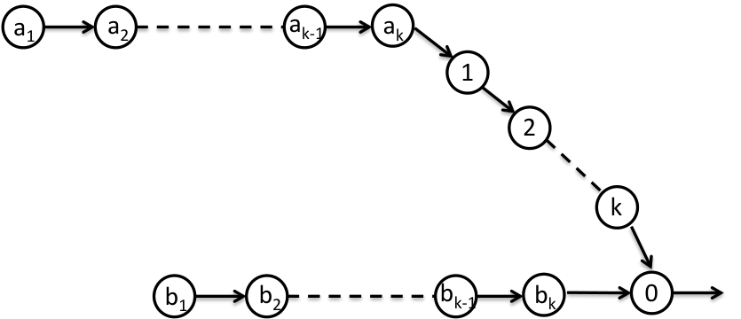
Consider a network example shown in Figure 5. The network has 3​k+13k+1 nodes where only node 00 is a destination; and ai,i∈{1,2,…,k}a_{i},i\in\{1,2,\ldots,k\} and bi,i∈{1,2,…,k}b_{i},i\in\{1,2,\ldots,k\} can have exogenous arrivals. Assume all link capacities are equal to 1; and the exogenous arrivals are periodic with period 2k, as follows:

  • •

    Time slot 11: One packet arrives at node a1a_{1}.

  • •

    Time slot 22: One packet arrives at node a2a_{2}.

  • •

    ⋯\cdots

  • •

    Time slot kk: One packet arrives at node aka_{k}.

  • •

    Time slot k+1k+1: One packet arrives at node b1b_{1}.

  • •

    Time slot k+2k+2: One packet arrives at node b2b_{2}.

  • •

    ⋯\cdots

  • •

    Time slot 2​k2k: One packet arrives at node bkb_{k}.

Under dynamics (7), each packet arrives on its own slot and traverses all links of its path to exit on the same slot it arrived. The queue backlog in each node is 00 for all time.

Under dynamics (8), the first packet arrives at time slot 11 to node a1a_{1}. This packet visits node a2a_{2} at time slot 22, when the second packet also arrives at a2a_{2}. One of these packets is delivered to node a3a_{3} at time slot 33, and another packet also arrives to node 33. The nodes {1,…,k}\{1,\ldots,k\} do not have any exogenous arrivals and act only to delay the delivery of all packets from the ai nodes. It follows that the link from node kk to node 00 will send exactly one packet over each slots t∈{2​k+1,2​k+2,…,2​k+k}t\in\{2k+1,2k+2,\ldots,2k+k\}. Similarly, the link from bkb_{k} to 00 sends exactly one packet to node 00 over each of these same slots. Thus, node 00 receives 22 packets on each slot t∈{2​k+1,2​k+2,…,2​k+k}t\in\{2k+1,2k+2,\ldots,2k+k\}, but can only output 11 packet per slot. The queue backlog in this node grows linearly and reaches k+1k+1 at time 2​k+k2k+k. Thus, the backlog in node 00 can be arbitrarily large when kk is large. This example demonstrates that, even when there is only one destination, the deviation between virtual queues under dynamics (7) and actual queues under dynamics (8) can be arbitrarily large, even when the in-degree and out-degree of 11 and an in-degree of at most 22.

Refer to caption
Fig. 5: An example illustrating the possibly large gap between queue model (7) and queue model (8)

Appendix C Proof of Part (2) in Lemma 1

Fix f∈ℱ,n∈𝒩∖{Dst​(f)}f\in\mathcal{F},n\in\mathcal{N}\setminus\{\text{Dst}(f)\}. By (10),

Q^n(f)​[t+1]\displaystyle\widehat{Q}_{n}^{(f)}[t+1]
=\displaystyle= max{Q^n(f)[t]−∑l∈𝒪⁡(n)μl(f)[t],0}+xf[t]𝟏{n=Src(f)}+∑l∈ℐ⁡(n)μl(f)[t]\displaystyle\max\big\{\widehat{Q}_{n}^{(f)}[t]-\sum_{l\in\mathcal{O}(n)}\mu_{l}^{(f)}[t],0\big\}+x_{f}[t]\mathbf{1}_{\{n=\text{Src}(f)\}}+\sum_{l\in\mathcal{I}(n)}\mu_{l}^{(f)}[t]
=\displaystyle= max{Q^n(f)[t]+xf[t]𝟏{n=Src(f)}+∑l∈ℐ⁡(n)μl(f)[t]−∑l∈𝒪⁡(n)μl(f)[t],xf[t]𝟏{n=Src(f)}+∑l∈ℐ⁡(n)μl(f)[t]}\displaystyle\max\Big\{\widehat{Q}_{n}^{(f)}[t]+x_{f}[t]\mathbf{1}_{\{n=\text{Src}(f)\}}+\sum_{l\in\mathcal{I}(n)}\mu_{l}^{(f)}[t]-\sum_{l\in\mathcal{O}(n)}\mu_{l}^{(f)}[t],~~x_{f}[t]\mathbf{1}_{\{n=\text{Src}(f)\}}+\sum_{l\in\mathcal{I}(n)}\mu_{l}^{(f)}[t]\Big\}
≥(a)\displaystyle\overset{(a)}{\geq} max{Q^n(f)[t]+xf[t]𝟏{n=Src(f)}+∑l∈ℐ⁡(n)μl(f)[t]−∑l∈𝒪⁡(n)μl(f)[t],0}\displaystyle\max\Big\{\widehat{Q}_{n}^{(f)}[t]+x_{f}[t]\mathbf{1}_{\{n=\text{Src}(f)\}}+\sum_{l\in\mathcal{I}(n)}\mu_{l}^{(f)}[t]-\sum_{l\in\mathcal{O}(n)}\mu_{l}^{(f)}[t],~~0\Big\}

where (a) follows from the fact that μl(f)​[t],xf​[t],∀f,l,t\mu_{l}^{(f)}[t],x_{f}[t],\forall f,l,t are non-negative. Note that the right side of the above equation is identical to the right side of (7) and recall that Yn(f)​[0]=0<Q^n(f)​[0]Y_{n}^{(f)}[0]=0<\widehat{Q}_{n}^{(f)}[0]. By inductions, we have Yn(f)​[t]≤Q^n(f)​[t],∀tY_{n}^{(f)}[t]\leq\widehat{Q}_{n}^{(f)}[t],\forall t. Since Q^n(f)​[t]=Qn(f)​[t]+B+∑l∈𝒪⁡(n)Cl,∀t\widehat{Q}_{n}^{(f)}[t]=Q_{n}^{(f)}[t]+B+\sum_{l\in\mathcal{O}(n)}C_{l},\forall t and Qn(f)​[t]≤B,∀tQ_{n}^{(f)}[t]\leq B,\forall t, we have Q^n(f)​[t]≤2​B+∑l∈𝒪⁡(n)Cl,∀t\widehat{Q}_{n}^{(f)}[t]\leq 2B+\sum_{l\in\mathcal{O}(n)}C_{l},\forall t. It follows that Yn(f)​[t]≤2​B+∑l∈𝒪⁡(n)Cl,∀tY_{n}^{(f)}[t]\leq 2B+\sum_{l\in\mathcal{O}(n)}C_{l},\forall t.

Appendix D Proof of Lemma 3

Note that problem (18)-(20) satisfies Slater’s condition. So the optimal solution to problem (18)-(20) is characterized by KKT conditions [22]. Introducing Lagrange multipliers θ∈ℝ+\theta\in\mathbb{R}_{+} for inequality constraint ∑k=1Kzk≤b\sum_{k=1}^{K}z_{k}\leq b and 𝝂=[ν1,…,νK]𝖳∈ℝ+K\boldsymbol{\nu}=[\nu_{1},\ldots,\nu_{K}]^{\mkern-1.5mu\mathsf{T}}\in\mathbb{R}_{+}^{K} for inequality constraints zk≥0,k∈{1,2,…,K}z_{k}\geq 0,k\in\{1,2,\ldots,K\}. Let 𝐳∗=[z1∗,…,zK∗]𝖳\mathbf{z}^{\ast}=[z_{1}^{\ast},\ldots,z_{K}^{\ast}]^{\mkern-1.5mu\mathsf{T}} and (θ∗,𝝂∗)(\theta^{\ast},\boldsymbol{\nu}^{\ast}) be any primal and dual pair with the zero duality gap. By KKT conditions, we have zk∗−ak+θ∗−νk∗=0,∀k∈{1,2,…,K};∑k=1Kzk∗≤b;θ∗≥0;θ∗​(∑k=1Kzk∗−b)=0;zk∗≥0,∀k∈{1,2,…,K};νk∗≥0,∀k∈{1,2,…,K};νk∗​zk∗=0,∀k∈{1,2,…,K}z_{k}^{\ast}-a_{k}+\theta^{\ast}-\nu_{k}^{\ast}=0,\forall k\in\{1,2,\ldots,K\};\sum_{k=1}^{K}z_{k}^{\ast}\leq b;\theta^{\ast}\geq 0;\theta^{\ast}\big(\sum_{k=1}^{K}z_{k}^{\ast}-b\big)=0;z_{k}^{\ast}\geq 0,\forall k\in\{1,2,\ldots,K\};\nu_{k}^{\ast}\geq 0,\forall k\in\{1,2,\ldots,K\};\nu_{k}^{\ast}z_{k}^{\ast}=0,\forall k\in\{1,2,\ldots,K\}.

Eliminating νk∗,∀k∈{1,2,…,K}\nu_{k}^{\ast},\forall k\in\{1,2,\ldots,K\} in all equations yields θ∗≥ak−zk∗,k∈{1,2,…,K};∑k=1Kzk∗≤b;θ∗≥0;θ∗​(∑k=1Kzk∗−b)=0;zk∗≥0,∀k∈{1,2,…,K};(zk∗−ak+θ∗)​zk∗=0,∀k∈{1,2,…,K}\theta^{\ast}\geq a_{k}-z_{k}^{\ast},k\in\{1,2,\ldots,K\};\sum_{k=1}^{K}z_{k}^{\ast}\leq b;\theta^{\ast}\geq 0;\theta^{\ast}\big(\sum_{k=1}^{K}z_{k}^{\ast}-b\big)=0;z_{k}^{\ast}\geq 0,\forall k\in\{1,2,\ldots,K\};(z_{k}^{\ast}-a_{k}+\theta^{\ast})z_{k}^{\ast}=0,\forall k\in\{1,2,\ldots,K\}.

For all k∈{1,2,…,K}k\in\{1,2,\ldots,K\}, we consider θ∗<ak\theta^{\ast}<a_{k} and θ∗≥ak\theta^{\ast}\geq a_{k} separately:

  1. 1.

    If θ∗<ak\theta^{\ast}<a_{k} , then θ∗≥ak−zk∗\theta^{\ast}\geq a_{k}-z_{k}^{\ast} holds only when zk∗>0z_{k}^{\ast}>0, which by (zk∗−ak+θ∗)​zk∗=0(z_{k}^{\ast}-a_{k}+\theta^{\ast})z_{k}^{\ast}=0 implies that zk∗=ak−θ∗z_{k}^{\ast}=a_{k}-\theta^{\ast}.

  2. 2.

    If θ∗≥ak\theta^{\ast}\geq a_{k}, then zk∗>0z_{k}^{\ast}>0 is impossible, because zk∗>0z_{k}^{\ast}>0 implies that zk∗−ak+θ∗>0z_{k}^{\ast}-a_{k}+\theta^{\ast}>0, which together with zk∗>0z_{k}^{\ast}>0 contradicts the slackness condition (zk∗−ak+θ∗)​zk∗=0(z_{k}^{\ast}-a_{k}+\theta^{\ast})z_{k}^{\ast}=0. Thus, if θ∗≥ak\theta^{\ast}\geq a_{k}, we must have zk∗=0z_{k}^{\ast}=0.

Summarizing both cases, we have zk∗=max⁡{0,ak−θ∗},∀k∈{1,2,…,K}z_{k}^{\ast}=\max\{0,a_{k}-\theta^{\ast}\},\forall k\in\{1,2,\ldots,K\}, where θ∗\theta^{\ast} is chosen such that ∑k=1Kzk∗≤b\sum_{k=1}^{K}z_{k}^{\ast}\leq b, θ∗≥0\theta^{\ast}\geq 0 and θ∗​(∑k=1Kzk∗−b)=0\theta^{\ast}\big(\sum_{k=1}^{K}z_{k}^{\ast}-b\big)=0.

To find such θ∗\theta^{\ast}, we first check if θ∗=0\theta^{\ast}=0. If θ∗=0\theta^{\ast}=0 is true, the slackness condition θ∗​(∑k=1Kzk∗−b)\theta^{\ast}\big(\sum_{k=1}^{K}z_{k}^{\ast}-b\big) is guaranteed to hold and we need to further require ∑k=1Kzk∗=∑k=1Kmax⁡{0,ak}≤b\sum_{k=1}^{K}z_{k}^{\ast}=\sum_{k=1}^{K}\max\{0,a_{k}\}\leq b. Thus θ∗=0\theta^{\ast}=0 if and only if ∑k=1Kmax⁡{0,ak}≤b\sum_{k=1}^{K}\max\{0,a_{k}\}\leq b. Thus, Algorithm 2 check if ∑k=1Kmax⁡{0,ak}≤b\sum_{k=1}^{K}\max\{0,a_{k}\}\leq b holds at the first step and if this is true, then we conclude θ∗=0\theta^{\ast}=0 and we are done!

Otherwise, we know θ∗>0\theta^{\ast}>0. By the slackness condition θ∗​(∑k=1Kzk∗−b)=0\theta^{\ast}\big(\sum_{k=1}^{K}z_{k}^{\ast}-b\big)=0, we must have ∑k=1Kzk∗=∑k=1Kmax⁡{0,ak−θ∗}=b\sum_{k=1}^{K}z_{k}^{\ast}=\sum_{k=1}^{K}\max\{0,a_{k}-\theta^{\ast}\}=b. To find θ∗>0\theta^{\ast}>0 such that ∑k=1Kmax⁡{0,ak−θ∗}=b\sum_{k=1}^{K}\max\{0,a_{k}-\theta^{\ast}\}=b, we could apply a bisection search by noting that all zk∗z_{k}^{\ast} are decreasing with respect to θ∗\theta^{\ast}.

Another algorithm of finding θ∗\theta^{\ast} is inspired by the observation that if aj≥ai,∀i,j∈{1,2,…,K}a_{j}\geq a_{i},\forall i,j\in\{1,2,\ldots,K\}, then zj∗≥zi∗z_{j}^{\ast}\geq z_{i}^{\ast}. Thus, we first sort all aka_{k} in a decreasing order, say π\pi is the permutation such that aπ⁡(1)≥aπ⁡(2)≥⋯≥aπ⁡(K)a_{\pi(1)}\geq a_{\pi(2)}\geq\cdots\geq a_{\pi(K)}; and then sequentially check if k∈{1,2,…,K}k\in\{1,2,\ldots,K\} is the index such that aπ⁡(k)−θ∗≥0a_{\pi(k)}-\theta^{\ast}\geq 0 and aπ⁡(k+1)−θ∗<0a_{\pi(k+1)}-\theta^{\ast}<0. To check this, we first assume kk is indeed such an index and solve the equation ∑j=1k(aπ⁡(j)−θ∗)=b\sum_{j=1}^{k}(a_{\pi(j)}-\theta^{\ast})=b to obtain θ∗\theta^{\ast}; (Note that in Algorithm 2, to avoid recalculating the partial sum ∑j=1kaπ⁡(j)\sum_{j=1}^{k}a_{\pi(j)} for each kk, we introduce the parameter Sk=∑j=1kaπ⁡(j)S_{k}=\sum_{j=1}^{k}a_{\pi(j)} and update SkS_{k} incrementally. By doing this, the complexity of each iteration in the loop is only O⁡(1)O(1).) then verify the assumption by checking if θ∗≥0\theta^{\ast}\geq 0, aπ⁡(k)−θ∗≥0a_{\pi(k)}-\theta^{\ast}\geq 0 and aπ⁡(k+1)−θ∗≤0a_{\pi(k+1)}-\theta^{\ast}\leq 0. The algorithm is described in Algorithm 2 and has complexity O⁡(K​log⁡(K))O(K\log(K)). The overall complexity is dominated by the step of sorting all aka_{k}.

Appendix E Proof of Lemma 6

The objective function (29) can be rewritten as

f⁡(𝐲)−∑f∈ℱ,n∈𝒩∖Dst​(f)(Wn(f)​[t]​gn(f)​(𝐲n(f))+αn​‖𝐲n(f)−𝐲n(f)​[t−1]‖2)−∑f∈ℱ,n=Dst​(f)αn​∑l∈ℐ⁡(n)(μl(f)−μl(f)​[t−1])2\displaystyle f(\mathbf{y})-\sum_{\begin{subarray}{c}f\in\mathcal{F},\\ n\in\mathcal{N}\setminus\text{Dst}(f)\end{subarray}}\big(W_{n}^{(f)}[t]g_{n}^{(f)}(\mathbf{y}_{n}^{(f)})+\alpha_{n}\|\mathbf{y}_{n}^{(f)}-\mathbf{y}_{n}^{(f)}[t-1]\|^{2}\big)-\sum_{f\in\mathcal{F},n=\text{Dst}(f)}\alpha_{n}\sum_{l\in\mathcal{I}(n)}(\mu_{l}^{(f)}-\mu_{l}^{(f)}[t-1])^{2}
=(a)\displaystyle\overset{(a)}{=} ∑f∈ℱUf(xf)−∑f∈ℱ,n∈𝒩∖Dst​(f)Wn(f)[t](xf𝟏{n=Src(f)}+∑l∈ℐ⁡(n)μl(f)−∑l∈𝒪⁡(n)μl(f))\displaystyle\sum_{f\in\mathcal{F}}U_{f}(x_{f})-\sum_{\begin{subarray}{c}f\in\mathcal{F},\\ n\in\mathcal{N}\setminus\text{Dst}(f)\end{subarray}}W_{n}^{(f)}[t]\Big(x_{f}\mathbf{1}_{\{n=\text{Src}(f)\}}+\sum_{l\in\mathcal{I}(n)}\mu_{l}^{(f)}-\sum_{l\in\mathcal{O}(n)}\mu_{l}^{(f)}\Big)
−∑f∈ℱ,n∈𝒩∖Dst​(f)αn((xf−xf[t−1])2𝟏{n=Src(f)}+∑l∈ℐ⁡(n)(μl(f)−μl(f)[t−1])2+∑l∈𝒪⁡(n)(μl(f)−μl(f)[t−1])2)\displaystyle-\sum_{\begin{subarray}{c}f\in\mathcal{F},\\ n\in\mathcal{N}\setminus\text{Dst}(f)\end{subarray}}\alpha_{n}\Big((x_{f}-x_{f}[t-1])^{2}\mathbf{1}_{\{n=\text{Src}(f)\}}+\sum_{l\in\mathcal{I}(n)}(\mu_{l}^{(f)}-\mu_{l}^{(f)}[t-1])^{2}+\sum_{l\in\mathcal{O}(n)}(\mu_{l}^{(f)}-\mu_{l}^{(f)}[t-1])^{2}\Big)
−∑f∈ℱ,n=Dst​(f)αn∑l∈ℐ⁡(n)(μl(f)−μl(f)[t−1])2\displaystyle-\sum_{f\in\mathcal{F},n=\text{Dst}(f)}\alpha_{n}\sum_{l\in\mathcal{I}(n)}(\mu_{l}^{(f)}-\mu_{l}^{(f)}[t-1])^{2}
=(b)\displaystyle\overset{(b)}{=} ∑f∈ℱ(Uf​(xf)−WSrc​(f)(f)​[t]​xf−αSrc​(f)​(xf−xf​[t−1])2)+∑(n,m)∈ℒ∑f∈ℱ(Wn(f)​[t]−Wm(f)​[t])​μ(n,m)(f)\displaystyle\sum_{f\in\mathcal{F}}\big(U_{f}(x_{f})-W_{\text{Src}(f)}^{(f)}[t]x_{f}-\alpha_{\text{Src}(f)}(x_{f}-x_{f}[t-1])^{2}\big)+\sum_{(n,m)\in\mathcal{L}}\sum_{f\in\mathcal{F}}\big(W_{n}^{(f)}[t]-W_{m}^{(f)}[t]\big)\mu_{(n,m)}^{(f)}
−∑(n,m)∈ℒ(αn+αm)∑f∈ℱ(μ(n,m)(f)−μ(n,m)(f)[t−1])2\displaystyle-\sum_{(n,m)\in\mathcal{L}}(\alpha_{n}+\alpha_{m})\sum_{f\in\mathcal{F}}(\mu_{(n,m)}^{(f)}-\mu_{(n,m)}^{(f)}[t-1])^{2} (31)

where (a) follows from the fact that gn(f)(𝐲n(f))=xf𝟏{n=Src(f)}+∑l∈ℐ⁡(n)μl(f)−∑l∈𝒪⁡(n)μl(f)g_{n}^{(f)}(\mathbf{y}_{n}^{(f)})=x_{f}\mathbf{1}_{\{n=\text{Src}(f)\}}+\sum_{l\in\mathcal{I}(n)}\mu_{l}^{(f)}-\sum_{l\in\mathcal{O}(n)}\mu_{l}^{(f)} and ∥𝐲n(f)−𝐲n(f)[t−1]∥2=(xf−xf[t−1])2𝟏{n=Src(f)}+∑l∈ℐ⁡(n)(μl(f)−μl(f)[t−1])2+∑l∈𝒪⁡(n)(μl(f)−μl(f)[t−1])2\|\mathbf{y}_{n}^{(f)}-\mathbf{y}_{n}^{(f)}[t-1]\|^{2}=(x_{f}-x_{f}[t-1])^{2}\mathbf{1}_{\{n=\text{Src}(f)\}}+\sum_{l\in\mathcal{I}(n)}(\mu_{l}^{(f)}-\mu_{l}^{(f)}[t-1])^{2}+\sum_{l\in\mathcal{O}(n)}(\mu_{l}^{(f)}-\mu_{l}^{(f)}[t-1])^{2}; and (b) follows by collecting each linear term μl(f)\mu_{l}^{(f)} and each quadratic term (μl(f)−μl(f)​[t−1])2(\mu_{l}^{(f)}-\mu_{l}^{(f)}[t-1])^{2}. Note that each link session rate μl(f)\mu_{l}^{(f)} appears twice with opposite signs in the summation term ∑f∈ℱ,n∈𝒩∖{Dst​(f)}Wn(f)[t](xf𝟏{n=Src(f)}+∑l∈ℐ⁡(n)μl(f)−∑l∈𝒪⁡(n)μl(f))\sum_{f\in\mathcal{F},n\in\mathcal{N}\setminus\{\text{Dst}(f)\}}W_{n}^{(f)}[t]\big(x_{f}\mathbf{1}_{\{n=\text{Src}(f)\}}+\sum_{l\in\mathcal{I}(n)}\mu_{l}^{(f)}-\sum_{l\in\mathcal{O}(n)}\mu_{l}^{(f)}\big) unless link ll flows into Dst​(f)\text{Dst}(f) and recall that WDst​(f)(f)=0,∀f∈ℱW_{\text{Dst}(f)}^{(f)}=0,\forall f\in\mathcal{F}. The quadratic terms are collected in a similar way. Note that the term ∑f∈ℱ,n=Dst​(f)αn​∑l∈ℐ⁡(n)(μl(f)−μl(f)​[t−1])2\sum_{f\in\mathcal{F},n=\text{Dst}(f)}\alpha_{n}\sum_{l\in\mathcal{I}(n)}(\mu_{l}^{(f)}-\mu_{l}^{(f)}[t-1])^{2} introduced to the objective function (29) is necessary to guarantee each quadratic term (μ(m,n)(f)−μ(m,n)(f)​[t−1])2(\mu_{(m,n)}^{(f)}-\mu_{(m,n)}^{(f)}[t-1])^{2} with the same link index (n,m)(n,m) but different flow indices f∈ℱf\in\mathcal{F} have the same coefficient αn+αm\alpha_{n}+\alpha_{m} in the last line of (31).

Note that equation (31) is now separable for each scalar xfx_{f} and vector [μ(n,m)(f)]f∈ℱ[\mu_{(n,m)}^{(f)}]_{f\in\mathcal{F}}. Thus, problem (29)-(30) can be decomposed into independent smaller optimization problems in the form of problem (12)-(13) with respect to each scalar xfx_{f}, and in the form of problem (14)-(17) with respect to each vector [μ(n,m)(f)]f∈ℱ[\mu_{(n,m)}^{(f)}]_{f\in\mathcal{F}}.

Appendix F Proof of Lemma 7

Note that Wn(f)​[t]W_{n}^{(f)}[t] appears as a known constant in (12). Since Uf​(xf)U_{f}(x_{f}) is concave and Wn(f)​[t]​xfW_{n}^{(f)}[t]x_{f} is linear, it follows that (12) is strongly concave with respect to xfx_{f} with modulus 2​αn2\alpha_{n}. Since xf​[t]x_{f}[t] is chosen to solve (12)-(13), by Lemma 4, ∀f∈ℱ\forall f\in\mathcal{F}, we have

Uf​(xf​[t])−WSrc​(f)(f)​[t]​xf​[t]−αn​(xf​[t]−xf​[t−1])2⏟(32)-I≥Uf​(xf∗)−WSrc​(f)(f)​[t]​xf∗−αn​(xf∗−xf​[t−1])2+αn​(xf∗−xf​[t])2⏟(32)-II.\displaystyle\underbrace{U_{f}(x_{f}[t])-W_{\text{Src}(f)}^{(f)}[t]x_{f}[t]-\alpha_{n}(x_{f}[t]-x_{f}[t-1])^{2}}_{\text{\eqref{eq:pf-dpp-bound-eq1}-I}}\geq\underbrace{U_{f}(x_{f}^{\ast})-W_{\text{Src}(f)}^{(f)}[t]x_{f}^{\ast}-\alpha_{n}(x_{f}^{\ast}-x_{f}[t-1])^{2}+\alpha_{n}(x_{f}^{\ast}-x_{f}[t])^{2}}_{\text{\eqref{eq:pf-dpp-bound-eq1}-II}}. (32)

Similarly, we know (14) is strongly concave with respect to vector [μ(n,m)f]f∈ℱ[\mu_{(n,m)}^{f}]_{f\in\mathcal{F}} with modulus 2​(αn+αm)2(\alpha_{n}+\alpha_{m}). By Lemma 4, ∀(n,m)∈𝒪⁡(n)\forall(n,m)\in\mathcal{O}(n), we have

∑f∈ℱ(Wn(f)​[t]−Wm(f)​[t])​μ(n,m)(f)​[t]−(αn+αm)​∑f∈ℱ(μ(n,m)(f)​[t]−μ(n,m)(f)​[t−1])2⏟(33)-I\displaystyle\underbrace{\sum_{f\in\mathcal{F}}\big(W_{n}^{(f)}[t]-W_{m}^{(f)}[t]\big)\mu_{(n,m)}^{(f)}[t]-\big(\alpha_{n}+\alpha_{m}\big)\sum_{f\in\mathcal{F}}\big(\mu_{(n,m)}^{(f)}[t]-\mu_{(n,m)}^{(f)}[t-1]\big)^{2}}_{\text{\eqref{eq:pf-dpp-bound-eq2}-I}}
≥\displaystyle\geq ∑f∈ℱ(Wn(f)​[t]−Wm(f)​[t])​μ(n,m)(f),∗−(αn+αm)​∑f∈ℱ(μ(n,m)(f),∗−μ(n,m)(f)​[t−1])2+(αn+αm)​∑f∈ℱ(μ(n,m)(f),∗−μ(n,m)(f)​[t])2⏟(33)-II.\displaystyle\underbrace{\sum_{f\in\mathcal{F}}\big(W_{n}^{(f)}[t]-W_{m}^{(f)}[t]\big)\mu_{(n,m)}^{(f),\ast}-\big(\alpha_{n}+\alpha_{m}\big)\sum_{f\in\mathcal{F}}\big(\mu_{(n,m)}^{(f),\ast}-\mu_{(n,m)}^{(f)}[t-1]\big)^{2}+\big(\alpha_{n}+\alpha_{m}\big)\sum_{f\in\mathcal{F}}\big(\mu_{(n,m)}^{(f),\ast}-\mu_{(n,m)}^{(f)}[t]\big)^{2}}_{\text{\eqref{eq:pf-dpp-bound-eq2}-II}}. (33)

Recall that each column vector 𝐲n(f)\mathbf{y}_{n}^{(f)} defined in (IV-B) is composed by control actions that appear in each constraint (2); column vector 𝐲=[xf;μl(f)]f∈ℱ,l∈ℒ\mathbf{y}=[x_{f};\mu_{l}^{(f)}]_{f\in\mathcal{F},l\in\mathcal{L}} is the collection of all control actions; and f⁡(𝐲)=∑f∈ℱUf​(xf)f(\mathbf{y})=\sum_{f\in\mathcal{F}}U_{f}(x_{f}). Summing term (32)-I over all f∈ℱf\in\mathcal{F} and term (33)-I over all (n,m)∈ℒ(n,m)\in\mathcal{L} and using an argument similar to the proof of Lemma 6 (Recall that 𝐲⁡[t]\mathbf{y}[t] is jointly chosen to minimize (29) by Lemma 6.) yields

∑f∈ℱ(32)-I+∑(n,m)∈𝒩 (33)-I\displaystyle\sum_{f\in\mathcal{F}}\text{\eqref{eq:pf-dpp-bound-eq1}-I}+\sum_{(n,m)\in\mathcal{N}}\text{ \eqref{eq:pf-dpp-bound-eq2}-I}
=\displaystyle= f⁡(𝐲⁡[t])−∑f∈ℱ,n∈𝒩∖Dst​(f)(Wn(f)​[t]​gn(f)​(𝐲n(f)​[t])+αn​‖𝐲n(f)​[t]−𝐲n(f)​[t−1]‖2)−∑f∈ℱ,n=Dst​(f)αn​∑l∈ℐ⁡(n)(μl(f)​[t]−μl(f)​[t−1])2.\displaystyle f(\mathbf{y}[t])-\sum_{\begin{subarray}{c}f\in\mathcal{F},\\ n\in\mathcal{N}\setminus\text{Dst}(f)\end{subarray}}\big(W_{n}^{(f)}[t]g_{n}^{(f)}(\mathbf{y}_{n}^{(f)}[t])+\alpha_{n}\|\mathbf{y}_{n}^{(f)}[t]-\mathbf{y}_{n}^{(f)}[t-1]\|^{2}\big)-\sum_{\begin{subarray}{c}f\in\mathcal{F},\\ n=\text{Dst}(f)\end{subarray}}\alpha_{n}\sum_{l\in\mathcal{I}(n)}(\mu_{l}^{(f)}[t]-\mu_{l}^{(f)}[t-1])^{2}. (34)

Recall that Φ[t]=∑f∈ℱ,n∈𝒩(αn𝟏{n≠Dst(f)}∥𝐲n(f),∗−𝐲n(f)[t]∥2+αn𝟏{n=Dst(f)}∑l∈ℐ⁡(n)(μl(f),∗−μl(f)[t])2)\Phi[t]=\sum_{f\in\mathcal{F},n\in\mathcal{N}}\big(\alpha_{n}\mathbf{1}_{\{n\neq\text{Dst}(f)\}}\|\mathbf{y}_{n}^{(f),\ast}-\mathbf{y}_{n}^{(f)}[t]\|^{2}+\alpha_{n}\mathbf{1}_{\{n=\text{Dst}(f)\}}\sum_{l\in\mathcal{I}(n)}(\mu_{l}^{(f),\ast}-\mu_{l}^{(f)}[t])^{2}\big). Summing term (32)-II over all f∈ℱf\in\mathcal{F} and term (33)-II over all (n,m)∈ℒ(n,m)\in\mathcal{L} yields

∑f∈ℱ(32)-II+∑(n,m)∈𝒩 (33)-II=f⁡(𝐲∗)+Φ⁡[t]−Φ⁡[t−1]−∑f∈ℱ,n∈𝒩∖Dst​(f)Wn(f)​[t]​gn(f)​(𝐲n(f),∗),\displaystyle\sum_{f\in\mathcal{F}}\text{\eqref{eq:pf-dpp-bound-eq1}-II}+\sum_{(n,m)\in\mathcal{N}}\text{ \eqref{eq:pf-dpp-bound-eq2}-II}=f(\mathbf{y}^{\ast})+\Phi[t]-\Phi[t-1]-\sum_{\begin{subarray}{c}f\in\mathcal{F},\\ n\in\mathcal{N}\setminus\text{Dst}(f)\end{subarray}}W_{n}^{(f)}[t]g_{n}^{(f)}(\mathbf{y}_{n}^{(f),\ast}), (35)

Combining (32)-(35) and rearranging terms yields

f⁡(𝐲⁡[t])\displaystyle f(\mathbf{y}[t])
≥\displaystyle\geq f⁡(𝐲∗)+Φ⁡[t]−Φ⁡[t−1]−∑f∈ℱ,n∈𝒩∖Dst​(f)Wn(f)​[t]​gn(f)​(𝐲n(f),∗)+∑f∈ℱ,n∈𝒩∖Dst​(f)(Wn(f)​[t]​gn(f)​(𝐲n(f)​[t])+αn​‖𝐲n(f)​[t]−𝐲n(f)​[t−1]‖2)\displaystyle f(\mathbf{y}^{\ast})+\Phi[t]-\Phi[t-1]-\sum_{\begin{subarray}{c}f\in\mathcal{F},\\ n\in\mathcal{N}\setminus\text{Dst}(f)\end{subarray}}W_{n}^{(f)}[t]g_{n}^{(f)}(\mathbf{y}_{n}^{(f),\ast})+\sum_{\begin{subarray}{c}f\in\mathcal{F},\\ n\in\mathcal{N}\setminus\text{Dst}(f)\end{subarray}}\big(W_{n}^{(f)}[t]g_{n}^{(f)}(\mathbf{y}_{n}^{(f)}[t])+\alpha_{n}\|\mathbf{y}_{n}^{(f)}[t]-\mathbf{y}_{n}^{(f)}[t-1]\|^{2}\big)
+∑f∈ℱ,n=Dst​(f)αn∑l∈ℐ⁡(n)(μl(f)[t]−μl(f)[t−1])2\displaystyle+\sum_{\begin{subarray}{c}f\in\mathcal{F},\\ n=\text{Dst}(f)\end{subarray}}\alpha_{n}\sum_{l\in\mathcal{I}(n)}(\mu_{l}^{(f)}[t]-\mu_{l}^{(f)}[t-1])^{2}
≥(a)\displaystyle\overset{(a)}{\geq} f⁡(𝐲∗)+Φ⁡[t]−Φ⁡[t−1]+∑f∈ℱ,n∈𝒩∖Dst​(f)(Wn(f)​[t]​gn(f)​(𝐲n(f)​[t])+αn​‖𝐲n(f)​[t]−𝐲n(f)​[t−1]‖2)\displaystyle f(\mathbf{y}^{\ast})+\Phi[t]-\Phi[t-1]+\sum_{\begin{subarray}{c}f\in\mathcal{F},\\ n\in\mathcal{N}\setminus\text{Dst}(f)\end{subarray}}\big(W_{n}^{(f)}[t]g_{n}^{(f)}(\mathbf{y}_{n}^{(f)}[t])+\alpha_{n}\|\mathbf{y}_{n}^{(f)}[t]-\mathbf{y}_{n}^{(f)}[t-1]\|^{2}\big)
=(b)\displaystyle\overset{(b)}{=} f⁡(𝐲∗)+Φ⁡[t]−Φ⁡[t−1]+∑f∈ℱ,n∈𝒩∖Dst​(f)(Qn(f)​[t]​gn(f)​(𝐲n(f)​[t])+gn(f)​(𝐲n(f)​[t−1])​gn(f)​(𝐲n(f)​[t])+αn​‖𝐲n(f)​[t]−𝐲n(f)​[t−1]‖2)\displaystyle f(\mathbf{y}^{\ast})+\Phi[t]-\Phi[t-1]+\sum_{\begin{subarray}{c}f\in\mathcal{F},\\ n\in\mathcal{N}\setminus\text{Dst}(f)\end{subarray}}\big(Q_{n}^{(f)}[t]g_{n}^{(f)}(\mathbf{y}_{n}^{(f)}[t])+g_{n}^{(f)}(\mathbf{y}_{n}^{(f)}[t-1])g_{n}^{(f)}(\mathbf{y}_{n}^{(f)}[t])+\alpha_{n}\|\mathbf{y}_{n}^{(f)}[t]-\mathbf{y}_{n}^{(f)}[t-1]\|^{2}\big) (36)

where (a) follows because gn(f)​(𝐲n(f),∗)=0,∀f∈ℱ,∀n∈𝒩∖Dst​(f),g_{n}^{(f)}(\mathbf{y}_{n}^{(f),\ast})=0,\forall f\in\mathcal{F},\forall n\in\mathcal{N}\setminus\text{Dst}(f), and ∑f∈ℱ,n=Dst​(f)αn​∑l∈ℐ⁡(n)(μl(f)​[t]−μl(f)​[t−1])2≥0\sum_{f\in\mathcal{F},n=\text{Dst}(f)}\alpha_{n}\sum_{l\in\mathcal{I}(n)}(\mu_{l}^{(f)}[t]-\mu_{l}^{(f)}[t-1])^{2}\geq 0; (b) follows from the fact that Wn(f)​[t]=Qn(f)​[t]+gn(f)​(𝐲n(f)​[t−1])W_{n}^{(f)}[t]=Q_{n}^{(f)}[t]+g_{n}^{(f)}(\mathbf{y}_{n}^{(f)}[t-1]).

Recall that u1𝖳​u2=12​u12+12​u22−12​(u1−u2)2u_{1}^{\mkern-1.5mu\mathsf{T}}u_{2}=\frac{1}{2}u_{1}^{2}+\frac{1}{2}u_{2}^{2}-\frac{1}{2}(u_{1}-u_{2})^{2} for any u1,u2∈ℝu_{1},u_{2}\in\mathbb{R}. Thus, for all f∈ℱ,n∈𝒩∖Dst​(f)f\in\mathcal{F},n\in\mathcal{N}\setminus\text{Dst}(f), we have

gn(f)​(𝐲n(f)​[t−1])​gn(f)​(𝐲n(f)​[t])=12​(gn(f)​(𝐲n(f)​[t−1]))2+12​(gn(f)​(𝐲n(f)​[t]))2−12​(gn(f)​(𝐲n(f)​[t−1])−gn(f)​(𝐲n(f)​[t]))2.\displaystyle g_{n}^{(f)}(\mathbf{y}_{n}^{(f)}[t-1])g_{n}^{(f)}(\mathbf{y}_{n}^{(f)}[t])=\frac{1}{2}\big(g_{n}^{(f)}(\mathbf{y}_{n}^{(f)}[t-1])\big)^{2}+\frac{1}{2}\big(g_{n}^{(f)}(\mathbf{y}_{n}^{(f)}[t])\big)^{2}-\frac{1}{2}\big(g_{n}^{(f)}(\mathbf{y}_{n}^{(f)}[t-1])-g_{n}^{(f)}(\mathbf{y}_{n}^{(f)}[t])\big)^{2}. (37)

Substituting (37) into (36) yields

f⁡(𝐲⁡[t])≥\displaystyle f(\mathbf{y}[t])\geq f⁡(𝐲∗)+Φ⁡[t]−Φ⁡[t−1]+∑f∈ℱ,n∈𝒩∖Dst​(f)(Qn(f)​[t]​gn(f)​(𝐲n(f)​[t])+12​(gn(f)​(𝐲n(f)​[t−1]))2+12​(gn(f)​(𝐲n(f)​[t]))2CLOSE\displaystyle f(\mathbf{y}^{\ast})+\Phi[t]-\Phi[t-1]+\sum_{\begin{subarray}{c}f\in\mathcal{F},\\ n\in\mathcal{N}\setminus\text{Dst}(f)\end{subarray}}\Big(Q_{n}^{(f)}[t]g_{n}^{(f)}(\mathbf{y}_{n}^{(f)}[t])+\frac{1}{2}\big(g_{n}^{(f)}(\mathbf{y}_{n}^{(f)}[t-1])\big)^{2}+\frac{1}{2}\big(g_{n}^{(f)}(\mathbf{y}_{n}^{(f)}[t])\big)^{2}
OPEN−12​(gn(f)​(𝐲n(f)​[t−1])−gn(f)​(𝐲n(f)​[t]))2+αn​‖𝐲n(f)​[t]−𝐲n(f)​[t−1]‖2)\displaystyle-\frac{1}{2}\big(g_{n}^{(f)}(\mathbf{y}_{n}^{(f)}[t-1])-g_{n}^{(f)}(\mathbf{y}_{n}^{(f)}[t])\big)^{2}+\alpha_{n}\|\mathbf{y}_{n}^{(f)}[t]-\mathbf{y}_{n}^{(f)}[t-1]\|^{2}\Big)
≥(a)\displaystyle\overset{(a)}{\geq} f⁡(𝐲∗)+Φ⁡[t]−Φ⁡[t−1]+∑f∈ℱ,n∈𝒩∖Dst​(f)(Qn(f)​[t]​gn(f)​(𝐲n(f)​[t])+12​(gn(f)​(𝐲n(f)​[t−1]))2+12​(gn(f)​(𝐲n(f)​[t]))2CLOSE\displaystyle f(\mathbf{y}^{\ast})+\Phi[t]-\Phi[t-1]+\sum_{\begin{subarray}{c}f\in\mathcal{F},\\ n\in\mathcal{N}\setminus\text{Dst}(f)\end{subarray}}\Big(Q_{n}^{(f)}[t]g_{n}^{(f)}(\mathbf{y}_{n}^{(f)}[t])+\frac{1}{2}\big(g_{n}^{(f)}(\mathbf{y}_{n}^{(f)}[t-1])\big)^{2}+\frac{1}{2}\big(g_{n}^{(f)}(\mathbf{y}_{n}^{(f)}[t])\big)^{2}
OPEN+(αn−12​βn2)​‖𝐲n(f)​[t]−𝐲n(f)​[t−1]‖2)\displaystyle+\big(\alpha_{n}-\frac{1}{2}\beta_{n}^{2}\big)\|\mathbf{y}_{n}^{(f)}[t]-\mathbf{y}_{n}^{(f)}[t-1]\|^{2}\Big)
≥(b)\displaystyle\overset{(b)}{\geq} f⁡(𝐲∗)+Φ⁡[t]−Φ⁡[t−1]+∑f∈ℱ,n∈𝒩∖Dst​(f)(Qn(f)​[t]​gn(f)​(𝐲n(f)​[t])+12​(gn(f)​(𝐲n(f)​[t]))2)\displaystyle f(\mathbf{y}^{\ast})+\Phi[t]-\Phi[t-1]+\sum_{\begin{subarray}{c}f\in\mathcal{F},\\ n\in\mathcal{N}\setminus\text{Dst}(f)\end{subarray}}\Big(Q_{n}^{(f)}[t]g_{n}^{(f)}(\mathbf{y}_{n}^{(f)}[t])+\frac{1}{2}\big(g_{n}^{(f)}(\mathbf{y}_{n}^{(f)}[t])\big)^{2}\Big) (38)

where (a) follows from the Fact 2, i.e., each gn(f)​(⋅)g_{n}^{(f)}(\cdot) is Lipschitz with modulus βn\beta_{n} and (b) follows because αn≥12​(dn+1)\alpha_{n}\geq\frac{1}{2}(d_{n}+1), βn≤dn+1\beta_{n}\leq\sqrt{d_{n}+1} and 12​(gn(f)​(𝐲n(f)​[t−1]))2≥0\frac{1}{2}\big(g_{n}^{(f)}(\mathbf{y}_{n}^{(f)}[t-1])\big)^{2}\geq 0.

Subtracting (27) from (38) and cancelling the common terms on both sides yields

−Δ⁡[t]+f⁡(𝐲⁡[t])≥f⁡(𝐲∗)+Φ⁡[t]−Φ⁡[t−1].\displaystyle-\Delta[t]+f(\mathbf{y}[t])\geq f(\mathbf{y}^{\ast})+\Phi[t]-\Phi[t-1].

References

  • [1] L. Tassiulas and A. Ephremides, “Stability properties of constrained queueing systems and scheduling policies for maximum throughput in multihop radio networks,” IEEE Transactions on Automatic Control, vol. 37, no. 12, pp. 1936–1948, 1992.
  • [2] M. J. Neely, “Dynamic power allocation and routing for satellite and wireless networks with time varying channels,” Ph.D. dissertation, Massachusetts Institute of Technology, 2003.
  • [3] L. Georgiadis, M. J. Neely, and L. Tassiulas, “Resource allocation and cross-layer control in wireless networks,” Foundations and Trends in Networking, 2006.
  • [4] M. J. Neely, Stochastic network optimization with application to communication and queueing systems. Morgan & Claypool Publishers, 2010.
  • [5] A. Eryilmaz and R. Srikant, “Joint congestion control, routing, and mac for stability and fairness in wireless networks,” IEEE Journal on Selected Areas in Communications, vol. 24, no. 8, pp. 1514–1524, 2006.
  • [6] A. L. Stolyar, “Maximizing queueing network utility subject to stability: Greedy primal-dual algorithm,” Queueing Systems, vol. 50, no. 4, pp. 401–457, 2005.
  • [7] X. Lin and N. B. Shroff, “Joint rate control and scheduling in multihop wireless networks,” in Proceedings of IEEE Conference on Decision and Control (CDC), 2004.
  • [8] J.-W. Lee, R. R. Mazumdar, and N. B. Shroff, “Opportunistic power scheduling for dynamic multi-server wireless systems,” IEEE Transactions on Wireless Communications, vol. 5, no. 6, pp. 1506–1515, 2006.
  • [9] M. J. Neely, E. Modiano, and C. E. Rohrs, “Dynamic power allocation and routing for time-varying wireless networks,” IEEE Journal on Selected Areas in Communications, vol. 23, no. 1, pp. 89–103, 2005.
  • [10] J. Liu, N. B. Shroff, C. H. Xia, and H. D. Sherali, “Joint congestion control and routing optimization: An efficient second-order distributed approach,” IEEE/ACM Transactions on Networking, vol. 24, no. 3, pp. 1404–1420, 2015.
  • [11] M. J. Neely, “Super-fast delay tradeoffs for utility optimal fair scheduling in wireless networks,” IEEE Journal on Selected Areas in Communications, vol. 24, no. 8, pp. 1489–1501, 2006.
  • [12] L. Huang, S. Moeller, M. J. Neely, and B. Krishnamachari, “LIFO-backpressure achieves near-optimal utility-delay tradeoff,” IEEE/ACM Transactions on Networking, vol. 21, no. 3, pp. 831–844, 2013.
  • [13] E. Wei, A. Ozdaglar, and A. Jadbabaie, “A distributed Newton method for network utility maximization–I: algorithm,” IEEE Transactions on Automatic Control, vol. 58, no. 9, pp. 2162–2175, 2013.
  • [14] M. Zargham, A. Ribeiro, and A. Jadbabaie, “Accelerated backpressure algorithm,” in Proceedings of IEEE Global Communications Conference (GLOBECOM), 2013.
  • [15] N. Parikh and S. Boyd, “Proximal algorithms,” Foundations and Trends in Optimization, vol. 1, no. 3, pp. 123–231, 2013.
  • [16] X. Lin and N. B. Shroff, “Utility maximization for communication networks with multipath routing,” IEEE Transactions on Automatic Control, vol. 51, no. 5, pp. 766–781, 2006.
  • [17] F. P. Kelly, A. K. Maulloo, and D. K. Tan, “Rate control for communication networks: Shadow prices, proportional fairness and stability,” Journal of the Operational Research Society, pp. 237–252, 1998.
  • [18] S. H. Low and D. E. Lapsley, “Optimization flow control—I: basic algorithm and convergence,” IEEE/ACM Transactions on Networking, vol. 7, no. 6, pp. 861–874, 1999.
  • [19] D. P. Bertsekas, A. Nedić, and A. E. Ozdaglar, Convex Analysis and Optimization. Athena Scientific, 2003.
  • [20] J. Duchi, S. Shalev-Shwartz, Y. Singer, and T. Chandra, “Efficient projections onto the l1l_{1}-ball for learning in high dimensions,” in Proceedings of International Conference on Machine learning (ICML), 2008.
  • [21] M. J. Neely, “A simple convergence time analysis of drift-plus-penalty for stochastic optimization and convex programs,” arXiv preprint arXiv:1412.079, 2014.
  • [22] S. Boyd and L. Vandenberghe, Convex Optimization. Cambridge University Press, 2004.