Towards prediction of rapid intensification in tropical cyclones with recurrent neural networks
Abstract
The problem where a tropical cyclone intensifies dramatically within a short period of time is known as rapid intensification. This has been one of the major challenges for tropical weather forecasting. Recurrent neural networks have been promising for time series problems which makes them appropriate for rapid intensification. In this paper, recurrent neural networks are used to predict rapid intensification cases of tropical cyclones from the South Pacific and South Indian Ocean regions. A class imbalanced problem is encountered which makes it very challenging to achieve promising performance. A simple strategy was proposed to include more positive cases for detection where the false positive rate was slightly improved. The limitations of building an efficient system remains due to the challenges of addressing the class imbalance problem encountered for rapid intensification prediction. This motivates further research in using innovative machine learning methods.
Index Terms:
Cooperative neuro-evolution, recurrent neural networks, back-propagation through time, rapid intensification, tropical cyclones.I Introduction
Rapid Intensification (RI) occurs when a tropical cyclone intensifies dramatically within a short period of time [1]. RI remains as one of the major challenges in tropical weather forecasting [2, 3, 4]. This challenge is partially due to limited understanding of the physical mechanisms in the change in the wind intensity of tropical cyclones [2, 5]. It has been reported that warm ocean temperatures and warm-ocean eddies influence the RI of tropical cyclones [6, 7]. An assessment on the relationship between sea surface temperature and cyclone wind-intensity revealed no direct relationship in 50 % of the cases studied [8]. A comprehensive review has been presented with a focus on RI [4] that considered the relationship of different types of cloud formations for cyclogenesis. Expert systems that feature computational intelligence methods have been deployed for automatic identification of weather systems [9] and modelling [10, 11], hence, they form major motivation for tackling RI.
Neural networks are computational intelligence methods that have gained recognition in application to time series prediction [12, 13, 13, 14]. They have been involved in cyclone prediction and modelling, however, they are not as popular in weather prediction systems when compared with statistical counterparts [15, 16, 10]. Although there has not been a comprehensive study, the back-propagation neural network has been applied for cyclone track prediction [17]. Related techniques have also been used in the area of cyclogenesis to predict tropical disturbances that developed into tropical storms [18].
Recurrent neural networks (RNNs) are dynamical systems, which makes them suitable for modelling temporal sequences [19]. Backpropagation-through-time (BPTT) which employs gradient descent has been widely used for training RNNs [20, 21, 22].
The forecast of the behaviour of cyclones is considered extremely important for avoiding casualties and mitigating damage to property [23, 24]. Cyclones behave differently in different ocean basins, hence meteorological offices around the world adapt to a combination of techniques to predict several interrelated features that include tracks, intensity, and accompanying rainfall [23, 25]. There has been a number of cyclone track prediction methods and models developed for various ocean basins [25]. Coevolutionary RNNs have been applied for cyclone track and wind intensity prediction problem for the South Pacific Ocean with promising results [26, 27], which motivates their application to the problem of RI.
There has been devastating impact in the countries that fall in the path of rapidly intensifying tropical cyclones. There has not been much work done to predict RI cases, which could be very useful in cyclone disaster management systems. A study of the factors that cause rapid intensification is also very important in order to make a robust prediction. Recently, RI was approached for modelling using coevolutionary recurrent neural networks on assumption that RI cases have been previously detected [28].Modelling RI refers to the ability of the prediction model to precisely give the value for intensification, i.e. by how many knots will the cyclone intensify in next 24 hours. Although there exists a number of challenges for modelling, however, detection is the most challenging as the number of cases are very small when compared to the entire dataset of cyclones that occurred in the particular region. This issue will be highlighted in this study and the challenges of detection will be given.
In this paper, an assessment is presented for the duration of the cyclones, the number of RI cases and relationship of the duration with the number of RI cases for the South Pacific and the South Indian Ocean regions. Recurrent neural networks are trained using back-propagation-through-time [20] to predict the occurrence of RI.
The rest of the paper is organised as follows. Section 2 gives a background of cyclones and RNNs. In Section 3, the proposed framework is presented, while Section 4 presents the experiments and results. Section 5 concludes the paper with the discussion of future work.
II Mythology: Recurrent Neural Networks for Rapid Intensification
II-A Background
Neural networks used for time series prediction are mainly characterized into feedforward and recurrent architectures [29]. Feedforward networks have one or more hidden layers that propagate information to the output layer. In contrast to feedforward networks, RNNs are dynamical systems whose next state and output depends on the current network state and input; this makes them suitable for modelling temporal sequences. The Elman RNN is a popular and efficient architecture that employs context units to store the output of the state neurons from the computation of the previous time steps [19]. Each layer contains neurons that propagate activation from one layer to the next by computing a transfer function of their weighted sum of inputs. The context layer is used for computation of present states as they contain information about the previous states as shown in Figure which is designed for the RI problem. The goal of the context layer is a mechanism to transfer information from the previous time step to the future step when presented with data from the present time step. The dynamics of the change of hidden state neuron activation’s in Elman RNN is given by Equation (1).
| (1) |
where and represent the output of the context state neuron and input neurons, respectively. and represent their corresponding weights; represents the number of input neurons while and represents the number of hidden and context layer neurons, respectively. is a sigmoid transfer function. Time refers to each data point of the time series sample used for prediction.
Neural networks learn by training on data using an algorithm that modifies the weights as directed by a learning objective for a particular application. The dataset is usually divided into a training set and a testing set. The goal of learning is to find the set of weights of the neural network on the given training data in order to achieve maximum performance on unseen data. This is done by adjusting the weights in the network according to a learning rule until a certain criterion is met, which is usually expressed in terms of the network output error or cost function.
II-B Proposed methodology
Rapid intensification is defined by an increase in wind intensity by 30 knots within 24 hours [30]. A system is needed that can detect and predict the occurrence of RI in the next 24 hours. We use the RNN to predict the occurrence of RI from past cases. This can be viewed as a boolean classification problem where a decision is made (positive or negative).
An overview of the RNN with the training data and the respective training algorithms is given in Figure 1.
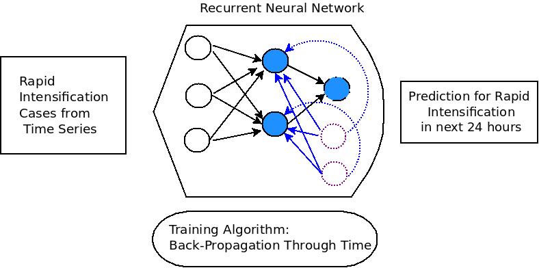
The cyclones used in this study are taken from the South Pacific and South Indian Ocean region [31]. The dataset contains times series information about the wind intensity, month, and track information in terms of longitude and latitude. The wind intensity for each cyclone is first analysed by a simple rule where a change within 24 hours is monitored for every point in the time series. If the wind intensity is greater than or equal to 30 knots within 24 hours, then the case is marked as positive, otherwise, it is negative. Note that each data point in the time series represents cyclone behavior taken at every six hours for regular intervals. Therefore, 30 hours of data is used for prediction.
The detection of RI is implemented using the following strategies. In Strategy I, all the positive cases are captured with RI greater than or equal to 30 knots and negative otherwise. Strategy II considers positive cases with RI greater than or equal to 10 knots and negative otherwise.
Table I shows that the number of positive cases of RI is a small portion when compared to negative cases, hence this is a class imbalance problem [32].
| Region | Dataset | No. Positive | No. Negative | Total |
|---|---|---|---|---|
| South Pacific | Training Set | 155 | 4798 | 4953 |
| Testing Set | 7 | 2002 | 2009 | |
| South Indian | Training Set | 190 | 6887 | 7077 |
| Testing Set | 70 | 6676 | 6746 |
RNNs can be trained with the principle of the delta learning rule. The general idea behind the delta learning rule is to use gradient descent to search the hypothesis space of the weight vectors and find the weights that best fit the set of training examples. Gradient descent is one of the most widely used RNN training in the implementation as backpropagation-through-time (BPTT) [20].
The BPTT algorithm unfolds a recurrent neural network in time into a deep multilayer feedforward network and employs the error backpropagation for weight update as shown in Algorithm 12. When unfolded in time, the network has the same behaviour as a recurrent neural network for a finite number of time steps.
III Analyses, Experiments and Results
This section presents analyses, experiments and results using RNNs for prediction RI cases in tropical cyclones. The Smart Bilo: computational intelligence framework implementation of BPTT for RNN is used for the respective experiments [33].
III-A Cyclone Dataset Analyses
The Southern Hemisphere tropical cyclone best-track data from Joint Typhoon Warning Center recorded every 6-hours is used as the main source of data [31]. We consider only the austral summer tropical cyclone season (November to April) from 1980 to 2013 data in the current study as data prior to the satellite era is not reliable due to inconsistencies and missing values. The South Indian basin domain is taken to be from 0-30∘S, 30∘E-130∘E and South Pacific domain is from 0-30∘S, 130∘E-130∘W.
The original data of tropical cyclone wind intensity in the South Pacific [31] was divided into training and testing set as follows:
- •
Training Set: Cyclones from 1985 - 2005 (219 Cyclones)
- •
Testing Set: Cyclones from 2006 - 2013 (71 Cyclones)
In the case for South Indian Ocean [31], the details are as follows:
- •
Training Set: Cyclones from 1985 - 2001 ( 285 Cyclones)
- •
Testing Set: Cyclones from 2002 - 2013 ( 190 Cyclones )
Figures 2 and 3 show the details of the duration of each cyclone in the training and test dataset for different cyclones given by their identification number (ID) on the x-axis. Note that each point of duration in the y-axis represents 6 hours. The second y-axis in the histogram
shows the number of cases of RI for each of the corresponding cyclones. These figures show the relationship between the number of cases of RI with their duration given by a number of hours. It is observed that in several cases,
the number of cases of RI does not directly relate to the duration of the cyclone. For instance, as shown in Figure 6 (b), Cyclone ID 20 has cyclone duration of about 50 6 hours. It contains about 6 cases of intensification whereas Cyclone ID 5 has a duration of 30 6 hours, which contains about 9 cases.
The number of RI cases in the South Indian Ocean is more than the South Pacific for both the training and testing dataset. This is due to the fact that the number of cyclones in the South Indian Ocean is more than the South Pacific.
III-B Detection of Rapid Intensification
The detection problem can be viewed as a classification problem that involves time series as input and a decision by the RNN whether it is a case of RI. The RNN is defined with the topology where 1 neuron is used in the input layer and 1 in the output layer. The RNN unfolds for time steps which are fixed at 5, this corresponds to the data points captured in 30 hours.
The extracted dataset is composed of positive and negative cases of RI in the training and test set as shown in Table I. The results for the detection (positive and negative cases) of RI in the South Pacific and South Indian Ocean region are given in Table II. Note that the results are given for two different strategies (Strategy I and II) which use 5 and 10 hidden neurons, respectively. In Strategy I, the distinction between positive and negative cases are made when rapid intensification is by 30 knows. This results in a highly unbalanced datasets which makes detection of true positives very difficult. Hence, Strategy II is used where the distinction between positive and negative cases is when rapid intensification is by 10 knots. In Strategy II, we achieve a bit poorer generalisation performance when compared to Strategy I, however, there is better detection of rapid intensification cases as shown by rate of true positives in Tables III - VI. These tables report the best result from the 30 experimental runs. The receiver operating characteristic (ROC) further describes the behaviour of the RNN detection system for Strategy II from best experimental run given in Figure 4. We note that the results show that the RI problem is very challenging and there is a need to improve the performance for detection of true positives with innovative strategies in learning unbalanced data sets.
| Problem | Strategy | Percentage (Test) |
|---|---|---|
| South Indian | I | 97.390 0.008 |
| South Indian | II | 81.736 0.219 |
| South Pacific | I | 97.214 0.013 |
| South Pacific | II | 79.779 0.169 |
| Predicted | ||||
| Positive | Negative | Total | ||
| Actual | Positive | |||
| Negative | ||||
| Total | ||||
| Predicted | ||||
| Positive | Negative | Total | ||
| Actual | Positive | |||
| Negative | ||||
| Total | ||||
| Predicted | ||||
| Positive | Negative | Total | ||
| Actual | Positive | |||
| Negative | ||||
| Total | 1876 | |||
| Predicted | ||||
| Positive | Negative | Total | ||
| Actual | Positive | |||
| Negative | ||||
| Total | 6369 | |||
III-C Discussion
After extraction of the cases for RI, it was determined that the detection problem features a class imbalanced problem that featured more than 98 % negative cases when RI of 30 knots was considered as Strategy I. Hence, Strategy II gathered more positive cases where RI of more than 10 knots was considered as positive. This lead to the RNN with more true positive cases when compared to Strategy I. However, the quality of detection becomes an issue when the difference between negative and positive cases is lowered from 30 to 10 knots.
Furthermore, BPTT has shown that the track of the cyclone is an important factor for modelling RI. The track information makes modelling RI a multi-variate time series problem. The comparison of the RNN performance with some of the prominent backpropagation algorithms from the literature shows that it is promising for the modelling phase. The experiments only considered 5 data points which are taken every 6 hours and spans for 30 hours. Better convergence could be obtained when more data points are available, i.e if cyclone readings are taken every 2 or 3 hours. Therefore, the proposed approach has faced the challenge of performing when given with limited data.
IV Conclusions and Future Work
This study first presented an analyses of RI cases in the South Pacific and South Indian Ocean region over the last three decades where it was shown that the number cases does not depend on the duration of the cyclone. The extraction of rapid intensification for the detection stage reported a class imbalanced problem that led to high rate of false positives. A simple strategy was proposed to include more positive cases for detection where the false positive rate was slightly improved. The limitations of building an efficient system remains due to the challenges of addressing the class imbalance problem encountered for rapid intensification prediction. This motivates further research in using innovative machine learning methods.
The prediction system could be improved further when more data is available. In addition, other factors such as the sea surface temperature, humidity and pressure levels could be incorporated to check if they contribute towards RI. These could further help in challenges to deal with the class imbalanced problem in the detection stage. Although RNNs were primarily used as the main model for detection, there is further scope for other learning algorithms. Further improvements for the detection stage could consider the use of ensemble methods such as bagging and boosting.
In future work, the proposed system can be used for cyclones and hurricanes in the rest of the regions such as the Atlantic Ocean. Machine learning paradigms such as transfer learning and multi-task learning could be used for improvement as a wide range of cyclone data from different regions are available that have distinct features in terms cyclone category, duration and decade or year of occurrence. Real-time implementation can be deployed through cloud computing infrastructure for computation and web services for mobile applications for disaster management.
References
- [1] C. R. Holliday and A. H. Thompson, “Climatological characteristics of rapidly intensifying typhoons,” Monthly Weather Review, vol. 107, pp. 1022–1034, 1979.
- [2] M. DeMaria, R. M. Zehr, J. P. Kossin, and J. A. Knaff, “The use of goes imagery in statistical hurricane intensity prediction,” in 25th Conference on Hurricanes and Tropical Meteorology, San Diego, CA, 2002, pp. 120 – 121.
- [3] B. Wang and X. Zhou, “Climate variation and prediction of rapid intensification in tropical cyclones in the western north pacific,” Meteorology and Atmospheric Physics, vol. 99, pp. 1 – 16, 2008.
- [4] J. Houze, R. A., “Clouds in tropical cyclones,” Mon. Wea. Rev, vol. 138, pp. 293–344, 2010.
- [5] J. M. Gross, “North atlantic and east pacific track and intensity verification for 2000,” in 55th Interdepartmental Hurricane Conference, Miami, FL. Office of the Federal Coordinator for Meteorological Services and Supporting Research, NOAA, B12–B15, 2002, pp. 120 – 121.
- [6] L. K. Shay, G. J. Goni, and P. G. Black, “Effects of a warm oceanic feature on hurricane opal,” Monthly Weather Review, vol. 128, pp. 1366–1383, 2000.
- [7] F. Oropeza and G. B. Raga, “Rapid deepening of tropical cyclones in the northeastern tropical pacific: The relationship with oceanic eddies,” Atmósfera, vol. 28, no. 1, pp. 27 – 42, 2015.
- [8] M. Ali, D. Swain, T. Kashyap, J. McCreary, and P. Nagamani, “Relationship between cyclone intensities and sea surface temperature in the tropical Indian Ocean,” Geoscience and Remote Sensing Letters, IEEE, vol. 10, no. 4, pp. 841–844, July 2013.
- [9] K. Y. Wong, C. L. Yip, and P. W. Li, “Automatic identification of weather systems from numerical weather prediction data using genetic algorithm,” Expert Systems with Applications, vol. 35, no. 1–2, pp. 542 – 555, 2008.
- [10] L. Zjavka, “Numerical weather prediction revisions using the locally trained differential polynomial network,” Expert Systems with Applications, vol. 44, pp. 265 – 274, 2016.
- [11] C.-C. Wei, “Wavelet kernel support vector machines forecasting techniques: Case study on water-level predictions during typhoons,” Expert Systems with Applications, vol. 39, no. 5, pp. 5189 – 5199, 2012.
- [12] Y. Zhao and S. Zhang, “Generalized dimension-reduction framework for recent-biased time series analysis,” Knowledge and Data Engineering, IEEE Transactions on, vol. 18, no. 2, pp. 231–244, Feb 2006.
- [13] W.-K. Wong, E. Bai, and A. Chu, “Adaptive time-variant models for fuzzy-time-series forecasting,” Systems, Man, and Cybernetics, Part B: Cybernetics, IEEE Transactions on, vol. 40, no. 6, pp. 1531–1542, Dec 2010.
- [14] M. Shen, W.-N. Chen, J. Zhang, H.-H. Chung, and O. Kaynak, “Optimal selection of parameters for nonuniform embedding of chaotic time series using ant colony optimization,” Cybernetics, IEEE Transactions on, vol. 43, no. 2, pp. 790–802, April 2013.
- [15] M. DeMaria and J. Kaplan, “A statistical hurricane intensity prediction scheme (ships) for the atlantic basin,” Weather Forecasting, vol. 9, pp. 209–220, 1994.
- [16] C. M. Rozoff and J. P. Kossin, “New probalistic forecast models for the prediction of tropical cyclone rapid intensification,” Weather and Forecasting, vol. 26, pp. 677 – 689, 2011.
- [17] Y. Wang, W. Zhang, and W. Fu, “Back propogation(bp)-neural network for tropical cyclone track forecast,” in Geoinformatics, 2011 19th International Conference on, June 2011, pp. 1–4.
- [18] N. Jaiswal and C. Kishtawal, “Prediction of tropical cyclogenesis using scatterometer data,” Geoscience and Remote Sensing, IEEE Transactions on, vol. 49, no. 12, pp. 4904–4909, Dec 2011.
- [19] J. L. Elman, “Finding structure in time,” Cognitive Science, vol. 14, pp. 179–211, 1990.
- [20] P. J. Werbos, “Backpropagation through time: what it does and how to do it,” Proceedings of the IEEE, vol. 78, no. 10, pp. 1550–1560, 1990.
- [21] Y. Bengio, P. Simard, and P. Frasconi, “Learning long-term dependencies with gradient descent is difficult,” IEEE Trans. Neural Networks, vol. 5, no. 2, pp. 157–166, 1994.
- [22] P. Frasconi, M. Gori, and A. Tesi, “Successes and failures of backpropagation: a theoretical investigation,” in Progress in Neural Networks. Ablex Publishing. Ablex Publishing, 1993, pp. 205–242.
- [23] “Tropical-cyclone forecasting: a worldwide summary of techniques and verification statistics,” Bulletin of American Meteorological Society, vol. 68.
- [24] G. Holland, “Global guide to tropical cyclone forecasting. bureau of meteorology research center, melbourne, australia,” http://cawcr.gov.au/publications/BMRC_archive/tcguide/globa_guide_intro.htm, 2009, accessed: January 21, 2015.
- [25] C. Roy and R. Kovordányi, “Tropical cyclone track forecasting techniques - a review,” Atmospheric Research, vol. 104-105, pp. 40–69, 2012.
- [26] R. Chandra and K. Dayal, “Cooperative coevolution of Elman recurrent networks for tropical cyclone wind-intensity prediction in the South Pacific region,” in IEEE Congress on Evolutionary Computtaion, Sendai, Japan, May 2015, pp. 1784–1791.
- [27] R. Chandra, K. Dayal, and N. Rollings, “Application of cooperative neuro-evolution of Elman recurrent networks for a two-dimensional cyclone track prediction for the South Pacific region,” in International Joint Conference on Neural Networks (IJCNN), Killarney, Ireland, July 2015, pp. 721–728.
- [28] R. Chandra and K. S. Dayal, “Coevolutionary recurrent neural networks for prediction of rapid intensification in wind intensity of tropical cyclones in the South Pacific region,” in International Conference on Neural Information Processing, ICONIP 2015, Istanbul, Turkey, November 9-12, 2015, Proceedings, Part III, 2015, pp. 43–52.
- [29] S. Haykin, Neural Networks and Learning Machines. Prentice Hall, 2008.
- [30] J. Kaplan and D. M., “Large-scale characteristics of rapidly intensifying tropical cyclones in the north atlantic basin,” Weather Forecasting, vol. 18, pp. 1093 – 1108, 2003.
- [31] (2015) JTWC tropical cyclone best track data site. [Online]. Available: http://www.usno.navy.mil/NOOC/nmfc-ph/RSS/jtwc/best_tracks/
- [32] N. Japkowicz and S. Stephen, “The class imbalance problem: A systematic study,” Intell. Data Anal., vol. 6, no. 5, pp. 429–449, 2002.
- [33] “Smart Bilo: Computational Intelligence Framework ,” accessed: 02-12-2015. [Online]. Available: smartbilo.aicrg.softwarefoundationfiji.org