Unified Models of Neutrinos, Flavour
and CP Violation
Abstract
Recent data from neutrino experiments gives intriguing hints about the mass ordering, the CP violating phase and non-maximal atmospheric mixing. There seems to be a (one sigma) preference for a normal ordered (NO) neutrino mass pattern, with a CP phase , and (more significantly) non-maximal atmospheric mixing. Global fits for the NO case yield lepton mixing angle one sigma ranges: , , . Cosmology gives a limit on the total of the three masses to be below about eV, favouring hierarchical neutrino masses over quasi-degenerate masses. Given such experimental advances, it seems an opportune moment to review the theoretical status of attempts to explain such a pattern of neutrino masses and lepton mixing, focussing on approaches based on the four pillars of: predictivity, minimality, robustness and unification. Predictivity can result from various mixing sum rules whose status is reviewed. Minimality can follow from the type I seesaw mechanism, including constrained sequential dominance of right-handed (RH) neutrinos, and the littlest seesaw model. Robustness requires enforcing a discrete CP and non-Abelian family symmetry, spontaneously broken by flavons with the symmetry preserved in a semi-direct way. Unification can account for all lepton and quark masses, mixing angles and CP phases, as in Supersymmetric Grand Unified Theories of Flavour, with possible string theory origin.
1 Introduction
Neutrino physics represents (at least so far) the first particle physics beyond the Standard Model (BSM). It gives tantalising new clues about the flavour puzzle which may lead to its eventual resolution. The importance of neutrino mass and mixing was recently acknowledged by the Nobel Prize for Physics in 2015, awarded to Takaaki Kajita for the Super-Kamiokande (SK) Collaboration and to Arthur B. McDonald for the Sudbury Neutrino Observatory (SNO) Collaboration. The citation was “for the discovery of neutrino oscillations, which shows that neutrinos have mass” and “for their key contributions to the experiments which demonstrated that neutrinos change identities”. Neutrino physics is the gift that keeps on giving, with new results and discoveries almost every year since 1998 [1, 2, 3]:
- •
1998 Atmospheric disappear, implying large atmospheric mixing (SK)
- •
2002 Solar disappear, implying large solar mixing (SK, after Homestake and Gallium)
- •
2002 Solar appear as and (SNO)
- •
2004 Reactor oscillations observed (KamLAND)
- •
2004 Accelerator disappear (K2K)
- •
2006 Accelerator disappearance confirmed and studied (MINOS)
- •
2010 Accelerator appear as (OPERA)
- •
2011 Accelerator appear as , hint for reactor mixing (T2K, MINOS)
- •
2012 Reactor disappear, and reactor angle measured (Daya Bay, RENO)
- •
2014 Accelerator appear as , hint for violation (T2K)
- •
2015 Various disappearance hints for Normal Ordering (SK, T2K, NOvA)
- •
2016 Accelerator disappearance “excludes maximal atmospheric mixing” (NOvA)
What have we learned from this wealth of data? We have learned that neutrinos have exceedingly small masses, all of them being much less than . Not a strong neutrino mass hierarchy, at least as compared to the charged lepton or quark masses. Neutrino masses break individual lepton numbers , however the jury is still out on whether they break total lepton number , which would be a signal that neutrinos are Majorana, rather than Dirac. Furthermore, neutrinos are observed to mix a lot, much more than the quarks; indeed the smallest lepton mixing angle is comparable to the largest quark mixing angle. In fact we have learned quite a lot about the lepton mixing angles and neutrino masses (or rather, their mass squared differences), as we shall discuss later. But before getting too carried away, it is worth summarising what we still don’t know:
- •
Is leptonic symmetry violated?
- •
Does belong to the first octant or the second octant?
- •
Are the neutrino mass squareds normal ordered (NO)?
- •
What is the lightest neutrino mass value?
- •
Are the neutrino masses of the Dirac or Majorana type?
Before entering into such details about the neutrino mass and mixing, and the emerging hints arising from the latest data for the what this pattern looks like, it is important the emphasise that we are dealing with BSM physics. To understand why this is evidence for BSM physics, we recall that, in the SM, neutrinos are massless for three reasons:
- •
There are no RH (sterile) neutrinos in the SM;
- •
In the SM there are no Higgs in triplet representations;
- •
The SM Lagrangian is renormalisable.
In the SM, there are three neutrinos , , which all massless and are distinguished by separate lepton numbers , , . The neutrinos and antineutrinos are distinguished by total lepton number . Clearly we must go beyond the SM to understand the origin of the tiny neutrino masses, so that at least one of the above should not apply.
For instance, if RH (sterile) neutrinos are included, then the usual Higgs mechanism of the SM yields Dirac neutrino mass in the same way as for the electron mass . This would break , , , but preserve . According to this simplest possibility, the Yukawa term would be , in the standard notation, and . By comparison, the electron mass has a Yukawa coupling eigenvalue of about .
Alternatively, neutrinos may have a Majorana mass which would break , leading to neutrinoless double beta decay. Indeed, having introduced RH neutrinos (also called sterile neutrinos, since they are SM singlets), something must prevent (large) Majorana mass terms where could take any value up to the Planck scale. A conserved symmetry such as would forbid RH neutrino masses, but if gauged (in order to be a robust symmetry) it would have to be broken at the TeV scale or higher, allowing Majorana masses at the breaking scale.
According to the above argument, SM singlet RH neutrino Majorana masses seem difficult to avoid. However, it is also possible to generate left-handed (LH) Majorana neutrino masses, which may arise even without RH neutrinos. Such masses are allowed below the electroweak (EW) scale since neutrinos do not carry electric charge. For instance, introducing a Higgs triplet (written as a matrix), LH Majorana neutrino masses arise from the term , where is a dimensionless coupling. Majorana masses occur once the lepton doublets are contracted with the neutral component of the Higgs triplet which develops a vacuum expectation value (VEV).
Alternatively, Majorana mass can arise from dimension five operators first proposed by Weinberg [4],
| (1) |
where is a dimensionless coupling constant, is a mass scale and is an triplet combination of two Higgs doublets (written as a matrix). This is a non-renormalisable operator, which is the lowest dimension operator which may be added to the renormalisable SM Lagrangian. We require for eV. The elegant type I seesaw mechanism [5] identifies the mass scale with the RH neutrino Majorana mass , and with the product of Dirac Yukawa couplings . Of course the situation is rather more complicated in practice since there may be three RH neutrinos and both and may be a matrices. In this case, after integrating out the RH neutrinos [5], we arrive at a more complicated version of Eq.1:
| (2) |
In general there are three classes of proposals in the literature for the new physics at the scale :
- •
- •
-parity violating supersymmetry [9] ( TeV Majorana mass neutralinos );
- •
Loop mechanisms involving scalars with masses of order the TeV-scale [10] (in which the Weinberg operator arises from loop diagrams involving additional Higgs doublets/singlets);
In addition there are two classes of early 11 1 We shall discuss some recent developments later. string-inspired explanations for neutrino mass:
In this review we shall focus on the type I seesaw mechanism (for a full discussion of other neutrino mass mechanisms see e.g. [13]). Whatever its origin, the observation of neutrino mass and mixing implies around seven new parameters beyond those in the SM, namely: 3 neutrino masses (or maybe 2 if one neutrino is massless), 3 lepton mixing angles, plus at least 1 phase which is violating. If there are 3 Majorana neutrino masses, then there will be 2 further violating phases. The existence of these extra seven (more or less) parameters, adding to the already twenty or so parameters of the minimal SM, means that we now have approaching thirty parameters describing our supposedly fundamental theory of quarks and leptons. In the words of Feynman [14]: “Nature gives us such wonderful puzzles! Why does She repeat the electron at 206 times and 3,640 times its mass?” Feynman goes on to say that there are many such numbers that are not understood, but although we use these numbers all the time we have no understanding of where they come from. He is of course referring to the flavour puzzle which is not addressed by the SM.
We define the flavour puzzle as a collection of related questions:
- •
What is the origin of the three lepton and quark families?
- •
Why are quark and lepton masses hierarchical?
- •
Why are quark masses the most hierarchical?
- •
Why are the two heavier neutrino masses less hierarchical?
- •
What is the theory behind the neutrino masses?
- •
Are neutrinos mainly Dirac or Majorana particles?
- •
Why are neutrino masses so small?
- •
What is the reason for large lepton mixing?
- •
What is the physics behind violation?
Neutrinos with mass and mixing exacerbates the flavour puzzle, but also provides fresh opportunities to resolve it. Indeed, as we shall see, the key observations are small neutrino masses and large lepton mixing. In this review article we shall be concerned with the impact of neutrino physics on models which address the flavour problem. We shall also consider how these theories fit into the quest for the unification of all particle forces, begun by Maxwell in his c.1865 unification of electricity and magnetism, and continued with the c.1965 electroweak unification of the SM.
To set the scene for the present review, let us briefly review neutrino model building, starting from 1998, as traced by a selection of earlier review articles [15, 16, 17, 18, 19, 20, 21, 22]. The earliest review [15] which considered models with both small and large solar mixing, with mass matrix textures enforced by a family symmetry, already considered how such models could be extended into Grand Unified Theories (GUTs). Another review [16], written shortly after large solar mixing was established in 2002, focussed on the idea of a seesaw mechanism in which there is a sequential dominance (SD) of the RH neutrinos [23, 24, 25], where a family symmetry such as [26] (continuous and non-Abelian) is required to simultaneously explain large solar and atmospheric mixing. The seesaw mechanism was also emphasised in [17]. It is worth emphasising that, back in the day, SD predicted a NO neutrino masses with (i.e. hierarchical as well as NO) and allowed a sizeable reactor angle [23, 24, 25], consistent with current data.
The next period in model building witnessed the rise of tri-bimaximal lepton mixing with a large number of such models being enforced by discrete non-Abelian family symmetries [27], enforced by vacuum alignment [28], as reviewed in [18, 19]. The discrete symmetry was linked to simple mixing patterns such as tri-bimaximal mixing. However, Nature turned out to be not so simple, and the discovery of a sizeable reactor angle in 2012 ruled out tri-bimaximal mixing, along with many of these models. Yet the idea of a simple discrete non-Abelian family symmetry survived, as exemplified by the post-2012 literature on models based on [29], [30] or [31].
Indeed, as the subsequent review articles [20, 21] showed, although tri-bimaximal lepton mixing is excluded, tri-bimaximal neutrino mixing is still possible in conjunction with charged lepton corrections. Another idea is to preserve either column 1 or 2 of the TB mixing matrix, called trimaximal ( or ) lepton mixing. In such cases the structures may still be enforced by discrete non-Abelian family symmetry. For example, several model building approaches were discussed in [20, 21] classified as: direct (involving a large discrete symmetry with a fixed reactor angle); semi-direct (with a small discrete symmetry but an undetermined reactor angle); indirect (again with a small discrete symmetry but novel vacuum alignments with a fixed reactor angle); or anarchy (no symmetry at all). Predictions of the phase resulting from the interplay of the discrete symmetry and the discrete family symmetry of semi-direct models were reviewed in [22]. The present situation in neutrino theory is a bit like an orchestra tuning up, with everyone playing a different tune. Hopefully this is just a prelude to a new movement in neutrino theory, as we will discuss in this review.
The present review will focus on classes of models which are based on the four pillars of:
- •
Predictivity (it must be possible to exclude such models by experiment);
- •
Minimality (models must be simple/elegant enough to have a chance of being correct);
- •
Robustness (models must be firmly based on some theoretical symmetry and/or dynamics);
- •
Unification (models must be capable of being embedded into a unified theory).
The first requirement of predictivity immediately excludes, for example, the idea of anarchy [32] which, along with many other flavour models, are not sufficiently predictive to enable them to be definitively tested. Similarly we shall regard models with very large discrete symmetry as failing the second test of minimality. Finally we consider ad hoc texture models based on mass matrices not enforced by symmetry, or models with unsubstantiated assumptions, as failing the third test of robustness. We also reject models which do not allow the gauge group to be unified. Examples of models which pass all four tests are the semi-direct models, mentioned above, based on smaller discrete symmetries, including those combined with spontaneous violation. Such models generally lead to mixing sum rules which can be subject to definitive experimental tests. There are a large number of such scenarios, based purely on symmetry arguments. We also go beyond symmetry arguments, and consider the dynamics of flavons (the Higgs which break the family symmetry) and the simplest type I seesaw mechanism, based on tree-level RH neutrino exchange. We show how such models may be extended to the quark sector, as well as the lepton sector, by embedding the Standard Model into a Supersymmetric Grand Unified Theory (SUSY GUT), augmented by a discrete non-Abelian family symmetry. Such models offer the promise of describing both quark and lepton masses, as well as their mixing angles and phases, in a single unified framework. Finally we speculate on the possible string theory origins of such theories, including gravity.
The layout of the remainder of this review is as follows. Following the pedagogical Introduction, in section 2 we give an overview of neutrino mixing and mass, including the latest global fits and the emerging hints from the latest neutrino data. The next four sections review the four pillars of: predictivity, minimality, robustness and unification. In section 3 on predictivity we describe some of the simpler ideas for lepton mixing, including the bimaximal, golden ratio and tri-bimaximal schemes. Although they are not viable by themselves, they may be corrected by charged lepton mixing, resulting in solar mixing sum rules. Alternatively, simple sub-structures may be partly preserved as in the case of trimaximal lepton mixing, resulting in atmospheric mixing rules. In section 4 on minimality we review the elegant type I seesaw mechanism, including the one RH neutrino (RHN) and two RHN models, as well as the idea of sequential dominance of three RH neutrinos, constrained sequential dominance and the littlest seesaw (LS) model. Section 5 on robustness is devoted to a brief review of discrete CP and non-Abelian family symmetry, spontaneously broken by flavons, in a semi-direct way. In section 6 on unification we briefly review GUTs and we then give examples of SUSY GUTs of flavour, which incorporate many of the preceding ideas, then speculate about the possible string theory origin of such theories. Section 7 concludes this review.
2 Neutrino Mass and Mixing
2.1 The Neutrino Parameters
Neutrino oscillation experiments are not sensitive absolute neutrino masses, only the neutrino mass squared differences:
| (3) |
There are two possible orderings, as shown in Fig.1, where the coloured bands indicate the probabilty that a particular neutrino mass eigenstate is composed of the various flavour or weak eigenstates , which are defined as the upper components of doublets in the diagonal charged lepton mass basis. One of the eigenstates is seen to contain roughly equal amounts of , which, if accurately realised, is known as bimaximal mixing. This (approximately) bimaximally mixed state may be either identifed as the heaviest mass eigenstate of mass (as shown in the left-half, called normal ordering (NO)) or such a state may be identified as the lightest one of mass (as shown in the right-half, called inverted ordering (IO)). One of the mass eigenstates is seen to contain roughly equal amounts of all three of the weak eigenstates , which, if accurately realised, is known as trimaximal mixing. Thus the neutrino mixing pattern is at least approximately characterised as being a tri-bimaximal mixing pattern, although reactor neutrino oscillation experiments in 2012 indicated a small but non-zero admixture of in the approximately bimaximally mixed state, so really the pattern of neutrino mixing should be referred to as a tri-bimaximal-reactor mixing pattern [33, 34].
The normal ordered (NO) pattern (positive ) seems to be slightly preferred by current data [3]. The best fit mass squared differences are: eV2 and eV2, according to the global fits [38, 39, 40], updated after Neutrino 2016 (and ICHEP 2016). These values and ranges are extracted from two of the updated global fits for the NO case as shown in Table 1. There is a cosmological limit on the sum total of the three neutrino masses: eV [35]. Prospects for future cosmological limits approaching this value are discussed in [36]. However, there is some cosmological model dependence in these determinations, as discussed in [36]. For a recent discussion of mass varying neutrinos which would evade these cosmological limits see [37]. In this review we shall sometimes focus on models with zero lightest neutrino mass. We stress that this is motivated purely by minimality rather than any definitive experimental indication. In this spirit, we note that, if , then NO would give eV and eV, hence eV. While for IO with , we would find eV, hence eV.
| NuFIT 3.0 | Capozzi et al | Range | |
| [∘] | |||
| [∘] | |||
| [∘] | |||
| [∘] | |||
| [] | |||
| [] |
Lepton mixing (analagous to similar mixing in the quark sector), may be parametrised by three lepton mixing angles. The lepton mixing matrix (assuming zero violation) relates the neutrino flavour or weak eigenstates (defined above) to the neutrino mass eigenstate basis states , according to: where is a real orthogonal rotation matrix in the plane, as shown in Eq.2.2 (with the phase set to zero) and depicted in Fig.2.
The measured mixing angles depend on whether the neutrino masses are in the NO or the IO pattern as shown in Fig.3. Tri-bimaximal mixing would correspond to and , and indicated by the dashed lines in Fig.3, which translates into , . The current best lepton mixing angle one sigma ranges are displayed in Table 1 for the NO case: , , . These values are extracted from the two recently updated global fits of [38, 39] 22 2 At the time of writing [40] has not yet been updated. The non-zero reactor angle excludes tri-bimaximal mixing. The alternative tri-bimaximal-reactor mixing is evidently excluded by about two sigma. In addition, there is weak evidence for a non-zero violating phase. Present data (slightly) prefers a normal ordered (NO) neutrino mass pattern, with a CP phase , and (more significantly) non-maximal atmospheric mixing. The meaning of the phase is discussed below.
2.2 Comparing the CKM and PMNS mixing matrices
The PDG [41] standardizes the parameterisation of the CKM and the PMNS mixing matrices in terms of unitary matrices consisting of a product of matrices :
where is the violating phase, relevant to the particular sector (either quark or lepton). We follow the short-hand notation , etc, with small quark mixing,
| (18) |
where the Wolfenstein parameter is [41]. From Table 1 we have large lepton mixing,
| (19) |
The smallest lepton mixing angle 33 3 When distinguishing leptons from quarks we use the superscripts and , but when it is obvious we are referring to leptons we often simply drop the superscript . (the reactor angle), is of order the largest quark mixing angle (the Cabibbo angle). There have been attempts to relate quark and lepton mixing angles such as postulating [42], however this relation is now experimentally excluded, along with all models which predicted this relation. This is a good example of how predictive models can be excluded by accurate experiments. Later we shall discuss other predictive models, some of which are excluded and some which are not yet excluded.
The violating quark phase , which is close to maximal 44 4 Interestingly, in Kobayashi-Maskawa’s parametrisation, is identified as the angle , where is one of the angles in the unitarity triangle corresponding to the and columns of the CKM matrix being orthogonal [41]., is reminiscent of the hint for the violating lepton phase .
2.3 Constructing the PMNS Lepton Mixing Matrix
In this subsection we discuss lepton mixing from first principles. For definiteness we consider Majorana masses, since Dirac neutrinos are completely analogous to the SM description of quarks. Consider the effective Lagrangian,
| (20) |
which is valid below the EW symmetry breaking scale, where are flavour indices. We do not yet specify the mechanism responsible for the above Majorana neutrino masses. The mass matrices may be diagonalised by unitary matrices,
The charged current (CC) couplings to in the flavour basis are given by , which becomes in the mass basis,
where we the lepton mixing matrix is identified as, 55 5 Different physically equivalent conventions appear in the literature, we follow the conventions in [25].,
| (33) |
It is possible to remove three of the lepton phases, using the phase invariance of . For example, , is unchanged by and . The three such phases may be chosen in various ways to yield an assortment of possible PMNS parametrisations one of which is the PDG standard choice discussed below). This does not apply to the Majorana mass terms where are real and positive, and thus the PMNS matrix may be parametrised as in Eq.2.2 but with an extra Majorana phase matrix [41]:
where and are irremovable Majorana phases. The mixing angles and must lie between and , while (after reordering the masses) lies between and . The phases all lie between and , however we shall equivalently express in the range to . There is no current constraint on the Majorana phases, and , nor is there likely to be in the forseeable future. The first step will be to experimentally show that neutrinos are Majorana particles, which will most likely require neutrinoless double beta decay to be discovered. Then, only after precision studies of neutrinoless double beta decay rates, will there be any hope of determining the Majorana phases and [43].
3 Predictivity: Lepton Mixing Patterns and Sum Rules
In this section we discuss some simple structures for . Although some are excluded by , they will motivate approaches which involve a non-zero . Others such as trimaximal mixing allow an undetermined reactor angle . An important point to emphasise is that all such ansatze may be enforced by a some small discrete non-Abelian family symmetry, making these predictions robust, as discussed in the following section.
3.1 Bimaximal and Golden Ratio Mixing
Bimaximal (BM) mixing is defined as and . It is sometimes enforced by . It corresponds to a matrix of the form [44],
| (41) |
3.2 Tri-bimaximal lepton mixing and deviation parameters
The Tribimaximal (TB) mixing matrix [47] is predicts and but differs since it predicts , i.e. . It may be enforced by , or sometimes with suitable field content. It corresponds to a mixing matrix,
| (43) |
It is excluded by , with and being more or less consistent. The deviation of the mixing angles from TB mixing may be parametrised as [48, 49]:
| (44) | |||||
| (45) | |||||
| (46) |
in terms of the ()olar, ()tmospheric and ()eactor deviation parameters. Current global fits for the NO case yield , , , which shows that the reactor angle represents the most significant deviation from TB mixing.
3.3 Trimaximal lepton mixing and sum rules
Trimaximal or lepton mixing preserves the first or the second column of Eq.43 [50],
| (47) |
The reactor angle is a free parameter. The unfilled entries are fixed when the reactor angle is specified. It is important to emphasise that these forms are more than simple ansatze, since they may be enforced by discrete non-Abelian family symmetry. For example, mixing can be realised by or symmetry [51], while mixing can be realised by symmetry [52]. A general group theory analysis of semi-direct symmetries was given in [53].
Eq.47 evidently implies the relations
| (48) | |||
| (49) |
The above relations above imply three equivalent relations:
| (50) |
leading to a prediction for , in agreement with current global fits, assuming . By contrast, the corresponding relations imply [50], which is in tension with current global best fit value . mixing also leads to an exact sum rule relation relation for in terms of the other lepton mixing angles [50],
| (51) |
which, for approximately maximal atmospheric mixing, predicts , or , in accord with the recent hints. Incidentally the reason why (not ) is predicted is because such predictions follow from being predicted, where , where are real functions of angles in Eq.2.2.
3.4 Charged lepton mixing corrections and sum rules
Recall that the physical PMNS matrix in Eq.33 is given by . Now suppose that is the TB matrix in Eq.43 while corresponds to small but unknown charged lepton corrections. This was first discussed in [55, 56, 57, 58] where the following sum rule involving the lepton mixing parameters, including crucially the phase , was first derived:
| (53) |
where . Eq.53 may be recast in terms of TB deviation parameters as [48],
| (54) |
To derive this sum rule, let us consider the case of the charged lepton mixing corrections involving only (1,2) mixing, so that the PMNS matrix is given by [58],
| (55) |
Comparing to the PMNS parametrisation in Eq.2.2 we identify the exact sum rule relations [58],
| (56) | |||||
| (57) | |||||
| (58) | |||||
| (59) |
The first equation implies a reactor angle if , just a little smaller than the Cabibbo angle. The second and third equations, after eliminating , yield a new relation between the PMNS parameters, , and . Expanding to first order gives the approximate solar sum rule relations in Eq.53 [55].
The above derivation assumes only (1,2) charged lepton corrections. However it is possible to derive an accurate sum rule which is valid for both (1,2) and (2,3) charged lepton corrections (while keeping ). Indeed, using a similar matrix multiplication method to that employed above leads to the exact result [59]:
| (60) |
This may also be obtained by taking the ratio of Eqs. 57 and 58. Therefore it applies to the previous case with . However, since cancels in the ratio, it also applies for . It is not fully general however since we are always assuming .
After some algebra, Eq.60 leads to [59],
| (61) |
To leading order in , Eq.61 returns the sum rule in Eq.53, from which we find if , consistent with . This can also be understood directly from Eq.61 where we see that for the leading terms and cancel in the numerator, giving to be compared to in the linear approximation. In general the error induced by using the linear sum rule instead of the exact one has been shown to be [59] for the TB sum rule.
Recently there has been much activity in exploring the phenomenology of various such solar mixing sum rules, arising from charged lepton corrections to simple neutrino mixing, not just TB neutrino mixing, but other simple neutrino mixing, including BM and GR mixing, allowing more general charged lepton corrections, renormalisation group running and so on [60].
It is important to distinguish solar mixing sum rules discussed here from atmospheric mixing sum rules discussed previously. The physics is different: here we consider charged lepton corrections to TB neutrino mixing, while previously we considered two forms of the physical trimaximal lepton mixing matrix.
4 Minimality: The Type I Seesaw Mechanism
4.1 The type I seesaw mechanism with one RH neutrino
The LH Majorana masses are given by,
| (62) |
where is a RH antineutrino field, which is the CP conjugate of the LH neutrino field . Majorana masses are possible below the electroweak symmetry (EW) breaking scale since the neutrino has zero electric charge. Majorana neutrino masses violate lepton number conservation, and are forbidden above the EW breaking scale. The type I seesaw mechanism assumes that Majorana neutrino mass terms are zero to begin with, but are generated effectively by RH neutrinos [5].
If we introduce one RH neutrino field , 77 7 A single RH neutrino is sufficient to account for atmospheric neutrino oscillations if it couples approximately equally to and as discussed in [23]. then there are two possible additional neutrino mass terms. First there are Majorana masses,
| (63) |
Secondly, there are Dirac masses,
| (64) |
Dirac mass terms arise from Yukawa couplings to a Higgs doublet, ,
| (65) |
where we write rather than in anticipation of a two Higgs doublet extension of the SM, with where .
Collecting together Eqs.63,64 (assuming Eq.62 terms to be absent) we have the seesaw mass matrix,
| (66) |
Since the RH neutrinos are electroweak singlets the Majorana masses of the RH neutrinos may be orders of magnitude larger than the electroweak scale. In the approximation that the matrix in Eq.66 may be diagonalised to yield effective Majorana masses of the type in Eq.62,
| (67) |
The seesaw mechanism formula is represented by the mass insertion diagram in Fig.4. This formula is valid below the EW scale. Above the EW scale, but below the scale , the seesaw mechanism is represented by the Weinberg operator in Eq.2, whose coefficient has the same structure as the seesaw formula in Eq.67.

The light effective LH neutrino Majorana mass is naturally suppressed by the heavy scale , but its precise value depends on the Dirac neutrino mass . Suppose we fix the desired physical neutrino mass to be eV, then the seesaw formula in Eq.67 relates the possible values of to as shown in Fig.5. This illustrates the huge range of allowed values of and consistent with an observed neutrino mass of 0.1 eV, with ranging from 1 eV up to the GUT scale, leading to many different types of seesaw models and phenomenology, including eV mass LSND sterile neutrinos, keV mass sterile neutrinos suitable for warm dark matter (WDM), GeV mass sterile neutrinos suitable for resonant leptogenesis and TeV mass sterile neutrinos possibly observable at the LHC (for a review see e.g. [61] and references therein). In this review we shall focus on the case of Dirac neutrino masses identified with charged quark and lepton masses, leading to a wide range of RH neutrino (or sterile neutrino) masses from the TeV scale to the GUT scale, which we refer to as the classic seesaw model. For example, if we take to be 1 GeV (roughly equal to the charm quark mass) then a neutrino mass of 0.1 eV requires a RH (sterile) neutrino mass of GeV.
4.2 The type I seesaw mechanism with two RH neutrinos
The type I see-saw neutrino model involving just two RH neutrinos was introduced in [24]. This is the minimal case sufficient to account for all neutrino oscillation data, and makes the prediction that the lightest neutrino mass is zero since the resulting light neutrino mass matrix is rank two [24]. In this case the neutrino masses are hierarchical (since the lightest mass is zero) and we can alternatively refer to normal ordered (NO) mass squareds as a normal hierarchy (NH) and inverted ordered (IO) mass squareds as an inverted hierarchy (IH).
Assuming the charged lepton mass matrix is diagonal, the two RH neutrinos and have Yukawa couplings [24],
| (68) |
where are the lepton doublets containing the mass eigenstates, and the VEV of the Higgs doublet. The Majorana Lagrangian is,
| (69) |
In the convention that the rows are and the columns are , we find the Dirac mass matrix,
| (70) |
The RH neutrino Majorana mass matrix with rows and columns is,
| (71) |
The see-saw formula in Eq.67 [5] gives a light neutrino mass matrix,
| (72) |
This is the effective Majorana mass matrix for LH neutrinos, and is the relevant mass matrix for the light neutrino states which appear dominantly in neutrino oscillations. The overall minus sign is not physical and can be safely dropped. In left-right (LR) convention, is the Dirac mass matrix. is the Majorana mass matrix, which typically involves masses higher than the EW scale. The physical neutrino mass matrix is obtained using the matrices in Eqs.70,71,
| (73) |
The main prediction of the two RH neutrino (2RHN) model is that the lightest neutrino mass is zero, but it does not distinguish between NO and IO, or make any further predictions. In order to make the 2RHN model more predictive one must make further assumptions. For example, the 2RHN model with two texture zeros [62] turns out to be only consistent with current data for the case of IO [63]. However the 2RHN model with one texture zero [24] is viable for the NO case.


4.3 The type I seesaw mechanism with three RH neutrinos and sequential dominance
More generally there may be three RH neutrinos, , and , with large Majorana masses and , respectively. They are sometimes called sterile neutrinos since they transform as singlets under the SM gauge group (see Fig.6). If the third RH neutrino makes a negligible contribution to the seesaw mechanism, either due to its high mass or its small Yukawa couplings , or both, then it will approximately decouple from the seesaw mechanism, and we return back to the two RH neutrino mass matrix in Eq.73. This decoupling may be part of a sequential dominance (SD) of the three RH neutrinos to the seesaw mechanism [23, 24],
| (74) |
At this stage, the SD condition in Eq.74 is just an assumption. However it may emerge in a robust way in the context of particular flavour models where the Yukawa couplings and RH neutrino masses are predicted from symmetry and dynamics, as is the case in the models discussed later. Eq.74 implies a strong and normal mass hierarchy:
| (75) |
where arises mainly from Fig.4 with exchange, while is dominated by exchange and the lightest neutrino mass arises from . The smallest physical neutrino mass vanishes in the limit that the primed couplings vanish, since then the model reduces to the two RH neutrino model in Eq.73 for which . Furthermore in the single RH neutrino approximation [23], we have . Hence SD in Eq.74 implies a normal neutrino mass hierarchy as in Eq.75 and Fig. 7. We emphasise that the prediction of a NH is two predictions: both NO and a hierarchy, specifically a very small value of lightest neutrino mass .
If in addition it is assumed that in the diagonal charged lepton mass basis, then Eq.74 implies [23, 24],
| (76) |
| (77) |
Eq.77, which shows that the reactor angle may be quite sizeable, was written down a decade before the angle was measured, and may be counted as a success of the SD approach. However to understand the reason why this bound is approximately saturated, we need to consider constrained forms of SD.
4.4 Constrained sequential dominance
In the previous subsection, we saw that a simple constraint on SD, namely in the diagonal charged lepton mass basis, led to some remarkably simple results for lepton mixing. One may go further and impose other constraints on the couplings (later enforced by symmetry) in order to enhance predictivity still further. The first example of such constrained sequential dominance (CSD) [55] was to impose the constraints , and leading to precise tri-bimaximal mixing. This can readily be seen by inserting these constrained Yukawa couplings into Eq.73, then showing that the resulting mass matrix is exactly diagonalised by the TB mixing matrix in Eq.43, as follows,
| (78) |
Although the above choice of Yukawa couplings leads to the undesirable result , other choices lead to values of reactor angle in agreement with experiment, while preserving the good values of atmospheric and solar mixing. The above CSD can be generalised to CSD() [64, 65, 66, 67, 68, 69, 70, 71, 72, 73] in which and (case A), or alternatively and (case B), for any postive integer . The other couplings are as before, and . Applying these constraints to Eq.70 gives,
| (79) |
The Dirac mass matrices above are is in the diagonal RH neutrino and charged lepton mass basis. According to Eq.76, we expect approximate TB mixing with these constraints applied. Exact analytic results for lepton mixing angles and phases based on CSD() have been derived in [71, 72]. The reactor angle has an approximate dependence of,
| (80) |
The predictions are sensitive to the relative phase between the complex masses and . 88 8 This is the only physical phase in the lepton sector of 2RHN CSD() models and as such may be identified with the leptogenesis phase, which requires a lightest RHN mass of GeV [70]. The choice returns us to the original CSD discussed at the start of this subsection, with a zero reactor angle. Choosing gives CSD(2) which fails to give a large enough reactor angle for all choices of phase [64]. The simplest viable case is CSD(3) [65], while CSD(4) is also possible [66, 67], and CSD() [69] is disfavoured due to the reactor angle being too large. In the next subsection we focus on the simplest viable case of CSD(3), with a fixed relative phase, which has been called the Littlest Seesaw (LS) [71, 72], since the resulting neutrino mass matrix involves the smallest number of free parameters. The theoretical justification for the constrained choice of Yukawa couplings relies of vacuum alignment and in particular symmetry as shown in [71, 72] and discussed later.
4.5 The Littlest Seesaw
The Littlest Seesaw (LS) model is the minimal viable seesaw model corresponding to a 2RHN model with CSD(). In the basis where the charged leptons have a diagonal mass matrix, and the RH neutrino mass matrix is also diagonal, CSD() corresponds to the Dirac mass matrix in Eq.79 with [65]:
| (81) |
After the seesaw mechanism has been implemented, the low energy effective LH Majorana neutrino mass matrix in the two RH neutrino case may be written as (see in Eq.73),
| (82) | ||||
| (83) |
where we have written and . The phase is physical: it is given by . The LS model is the minimal currently viable seesaw model since it involves only three real parameters . These parameters fix the three neutrino masses (one of which is zero) and fully determine the PMNS matrix (three angles and three phases, one of which is unphysical due to the zero neutrino mass).
Both LSA and LSB allow good fits of current data [74] as seen in Figure 8. The intersection of the accurately measured reactor angle one sigma band (in red) with the accurarely measured mass ratio one sigma band (in green) is instrumental in determining the model parameters and . There is a mild tension at the one sigma level with the less accurarely measured atmospheric and solar angles, so a better future determation of these angles could exclude the model. The best fit points in Figure 8 indicated by stars are close to and .
In Table 2, we show the best fit values of and with either free or held fixed at , together with the corresponding values of mixing parameters. The results are taken from [74] where more details may be found.

| LSA | LSB | NuFIT 3.0 | |||
| free | fixed | free | fixed | global fit | |
| [meV] | 27.22 | 26.78 | 27.14 | 26.77 | |
| [meV] | 2.653 | 2.678 | 2.658 | 2.681 | — |
| [rad] | |||||
| [∘] | 34.37 | 34.34 | 34.36 | 34.33 | |
| [∘] | 8.45 | 8.58 | 8.48 | 8.59 | |
| [∘] | 45.01 | 45.69 | 44.87 | 44.30 | |
| [∘] | -89.9 | -87.0 | -90.6 | -93.1 | |
| [] | 7.499 | 7.362 | 7.482 | 7.379 | |
| [] | 2.505 | 2.515 | 2.505 | 2.515 | |
| / d.o.f | 4.7 / 3 | 6.4 / 4 | 4.5 / 3 | 5.1 / 4 | — |
Both LSA and LSB both predict a NO neutrino mass pattern with a zero neutrino mass, , and lepton mixing as in Eq.47. To understand this, first observe that,
| (84) |
These equations show that the column vectors on the left are eigenvectors with zero eigenvalues, and in each case they may be identified as the first column of the PMNS mixing matrix associated with the zero neutrino mass , yielding the mixing form as in Eq.47. 99 9 In fact a NH neutrino mass pattern with a zero neutrino mass, , and lepton mixing is a prediction of all CSD() 2RHN seesaw models, by a similar argument. It can readily be verified that the best fit predictions in Table 1 respect the mixing sum rules in Eqs.50, 51.
The baryon asymmetry of the Universe (BAU) resulting from leptogenesis has the right sign, consistent with an excess of matter over antimatter, only if the lightest RH neutrino is , so that . It was estimated for LSA [70]:
| (85) |
Using (preferred by the fit with ), the correct baryon asymmetry requires,
| (86) |
Note that , which is the phase in the neutrino mass matrix in Eq.82, is also the leptogenesis phase in Eq.85. There is only one phase in LSA which controls everything: violation in the laboratory and in the Universe. This is a very attractive feature of the LS model.
For LSB, using (preferred by the fit with ) in order to achieve a positive matter-antimatter asymmetry we would require the lightest RH neutrino to be , so that [72].
Renormalisation group (RG) corrections have been studied for LSA and LSB with both and [73]. 1010 10 For a recent review of RG corrections in general neutrino mass models, with original references see e.g. [76]. It has been shown that, if the predictions in Table 2 are valid at high energies, such as the GUT scale, then the low energy angles are rather stable under radiative corrections. For example, the atmospheric angle receives corrections of [73], with the effect of radiative corrections tending to increase the low energy atmospheric angle compared to its GUT scale prediction.
4.6 Precision neutrino experiments vs the Littlest Seesaw
In the previous subsection we saw that both versions of the Littlest Seesaw, LSA and LSB, are consistent with current neutrino oscillation data. We noted that the well measured neutrino mass squared differences, when combined with the accurately determined reactor angle , were sufficient to precisely fix the parameters of the model , and . However we also saw that there is a mild tension at the one sigma level with the less accurarely measured atmospheric and solar angles, so a better future determation of these angles by future experiments could exclude the model.
This raises the general question of how precise experimental measurements need to be before qualitative progress can be made for flavour models. This type of input is very important to the experimental community and it can be fully addressed within a particular model such as the Littlest Seesaw. Indeed the prospects for excluding LSA and LSB in future neutrino oscillation experiments have recently been analysed [74], and we shall briefly review the results of that study. We should say at the outset that one way to exclude the LS models is via its prediction of a NO mass spectrum with . For example a determination of an IO would exclude these models, as would any signal from neutrinoless double beta decay experiments, or cosmology, which are not currently capable of seeing a signal for . In the following we assume that data continues to be consistent with such a neutrino mass spectrum and consider the prospects for excluding the models by precision measurements of the two mass squared differences, the three angles and the violating oscillation phase .
We shall focus on the future precision neutrino oscillation experiments Daya Bay, JUNO, DUNE and T2HK, as recently discussed in [75]. First we briefly summarise the plans for these experiments. Daya Bay is a short baseline neutrino oscillation experiment which detects anti-electron neutrinos from various nuclear reactors in China at distances between 1.5 km and 1.9 km, near the first atmospheric oscillation maxiimum. Daya Bay has currently the best precision on and in the future aims to acheive an accuracy of about 3% . JUNO is a medium baseline reactor experiment planned to have a basline of 53 km from two planned nuclear reactors in China, corresponding to the first solar oscillation maximum. The longer baseline would allow sensitive measurements of and accurate to about 0.5% . DUNE is a long baseline experiment which would use an accelerator at Fermilab to direct a wide band beam of muon (anti-)neutrinos with energies between 0.5 GeV and 5 GeV which are observed using a liquid Argon detector at Sanford located at a distance of 1300 km, near the first atmospheric oscillation maximum. T2HK is also a long baseline experiment which would use an accelerator at Tokai to direct a narrow 2.5 degree off-axis beam of muon (anti-)neutrinos with energies around 0.6 GeV which are observed using large water Cerenkov detectors in Kamioka located at a distance of 295 km, near the first atmospheric oscillation maximum. The muon disappearance and electron appearance channels of both DUNE and T2HK allow precise measurements of , the sign and magnitude of and the phase . In Figure 9 we show the prospects for excluding the Littlest Seesaw models using data from these future precision neutrino oscillation, where the top three panels show that JUNO, DUNE and T2HK are capable of excluding LSA and LSB over much of the currently allowed range of the solar and atmospheric angles and the phase.
5 Robustness: Discrete non-Abelian family symmetry models

5.1 Finite group theory

For a comprehensive introduction to (finite) group theory we refer the reader to [19]. Here we shall only recall a few basic features.
- •
A finite group contains of a finite number of elements together with a multiplication law between any two of the elements so that it yields another element of .
- •
A group must include the identity element .
- •
For every element there must be an inverse .
- •
The product of three elements satisfies (associative).
- •
Groups are called Abelian if all the elements commute, . Non-Abelian groups have elements which do not commute.
Abelian groups such as have elements which commute and may be represented by complex numbers, of unit modulus. Some non-Abelian groups subgroups of which contain triplet representations are depicted in Fig. 10. The simplest groups , [27], (in pale blue) are related to BM, TB and GR mixing. is an example of the series [77], while [78] is an example of the series [79]. , also called [80], is a simple group, with a subgroup [81]. For example, is the rigid rotation group of a cube, while is that of the tetrahedron, where is a subgroup of , as seen geometrically by inscribing the tetrahedron inside the cube as shown in Fig.11.
For a tetrahedron, there are twelve independent transformations (group elements of ) as follows (see Fig.11):
- •
4 rotations by 120∘ clockwise (about axes like AB) which are -type
- •
4 rotations by 120∘ anti-clockwise (about axes like AB) which are -type
- •
3 rotations by 180∘ (about axes like CD) which are -type
- •
1 unit operatator
For a cube there are 24 independent transformations (group elements of ) of which 12 are symmetries of (as above) and the remaining 12 are not symmetries of and are as follows (see Fig.11):
- •
3 rotations by 90∘ clockwise (about axes like CD)
- •
3 rotations by 90∘ anti-clockwise (about axes like CD)
- •
6 rotations by 180∘ (about axes like EF) which are -type
Although a group is specified by its multiplication table, the definition of a finite group this way becomes unweildy with increasing order (number of group elements) of . Another way is to use the “presentation” of the group, where the generators (subsets of elements from which all elements of the group can be obtained by multiplication) have to respect certain rules. For example, the permutation group of four objects , which is equivalent to the rigid symmetry group of the cube, can be defined by the presentation rules [82],
| (87) |
where , and are the three generators. If we drop , this reduces to the presentation of [27]. All the 24 group elements of may be obtained by multiplying the generators together, using the rules above. Similarly, all the 12 group group elements of may be obtained by multiplying the generators and together, subject to the above rules.
The main interest of group theory from the point of view of physics, is that the group elements may be represented by matrices which respect the group multiplication laws. The smallest such matrices which are not reducible to block diagonal form by a similarity transformation are called irreducible representations of the group. There are precise group theory rules for establishing the irreducible representations of any group, but here we shall only state the results for and in the -diagonal basis, see [19] for proofs, other examples and bases.
For there are two triplet matrix representations denoted and which are independent and irreducible. There are two singlet representations and . There also exists one irreducible doublet representation . For the subgroup there are three singlets and and one triplet . The matrix representations in the diagonal basis are given in the Table in Eq.88 [20] (where ). The Kronecker product rules for and are listed in Appendix A.
| (88) |
5.2 Klein symmetry and direct models
Suppose that the leptonic Lagrangian is invariant under the flavour symmetry associated with the group . Let us focus on the tranformations of the lepton doublet fields , where is spacetime and are the left-handed neutrino and charged lepton fields in a weak basis. The lepton doublets transform under as,
| (89) |
where is the group symmetry transformation matrix associated with the group element . For example if , and transforms as a triplet of , then is the three dimensional matrix form of in Eq.88, namely .
The diagonal charged lepton mass matrix , appearing in the Lagrangian term , may be combined into so that the right-handed transformations cancel, and there is a phase symmetry,
| (90) |
where for brevity we have written which generates a subgroup of .
In a similar way, the Klein symmetry of the neutrino mass matrix, in this basis, is given by,
| (91) |
where [83]
| (92) | |||
| (93) | |||
| (94) |
and
| (95) |
is called the Klein symmetry . For the case that is equal to the tri-bimaximal mixing matrix in Eq.43, then , and may be identified as the generators of in Eq.88. In this way one may associate TB mixing with the discrete symmetry group . However, if the mixing matrix is something other than then and will differ from the generators in Eq.88 and one must look for some other group. This exemplifies the so called “direct” approach to model building whereby one postulates a discrete symmetry group , whose generator enforces the diagonal charged lepton mass matrix, while its generators and enforce a particular Klein symmetry associated with a particular PMNS matrix. Different groups and generator embeddings will yield different predictions for the PMNS matrix.
From a dynamical point of view, the theory must organise itself so that the discrete symmetry group is broken by Higgs fields which know about flavour and are called flavons. The flavons may be EW singlets or doublets. There may be flavons whose VEVs preserve (i.e. ) and other whose VEVs preserve (i.e. and ). For example, consider the case of in the diagonal basis of Eq.88 [20], where we emphasise that:
| (96) |
In this basis one can check by explicit matrix multiplication (e.g. , where is the matrix in Eq.88 and is the column vector given below) that the symmetry preserving vacuum alignments are as follows [72]:
and the two important preserving alignments for flavons,
| (97) |
| (98) |
These flavons (identified with one or more of the preserving flavons) only carefully engineered to only appear in terms responsible for charged lepton masses. The other flavons (identified with one or more of the preserving flavons) only couple to terms responsible for neutrino masses.
This is the so called “direct approach” illustrated in Fig.12. For example can lead to TB mixing if is preserved in the charged lepton sector, and are preserved in the neutrino sector, which can be achieved dynamically by assuming that different symmetry preserving flavons are confined to a particular sector. For example the charged lepton mass matrix may arise from a non-renormalisable Lagrangian term where is a heavy mass scale once the flavon and Higgs get VEVs. Since only (not ) appears in the charged lepton sector, the mass matrix therefore respects the symmetry (see Eq.90) preserved by the VEV. Similarly respects the symmetry (see Eq.91) preserved by the VEV.
In such a “direct approach” the full Klein symmetry of the neutrino mass matrix arises as a subgroup of the initial family symmetry . Given the measurement of the reactor angle, the only viable direct models are those based on [85, 86, 84], with quite large required. Such models generally predict mixing and a phase , both of which are disfavoured by current data.
5.3 Semi-direct models
In the “semi-direct” approach, one may use smaller discrete family groups such as or . If applied in a “direct” way, such groups would lead to either TB or BM (for ) or GR mixing (for ), as in Fig.13. To obtain a non-zero reactor angle, one of the generators or must be broken. Thus the semi-direct models do not enforce the full residual symmetry.
Consider the following two interesting possibilities depicted in Fig.13:
- 1.
The symmetry of the charged lepton mass matrix is broken, but the full Klein symmetry in the neutrino sector is respected. This corresponds to having charged lepton corrections, with solar sum rules discussed in section 3.4.
- 2.
The symmetry of the neutrino mass matrix is broken, but the symmetry of the charged lepton mass matrix is unbroken. In addition either or (with being the product of and ) is preserved. This leads to either mixing (if is preserved); or mixing (if is preserved). Then we have the atmospheric sum rules as discussed in section 3.3.
In there is no generator to start with, but it is possible that preserved. This could also arise of is broken to at higher order [51]. In such cases, only half the Klein symmetry is preserved, corresponding to the generator of or , together with the symmetry of the diagonal generator enforcing the diagonality of the charged lepton mass matrix. However, the generator implies mixing and sum rules which are disfavoured due to the solar angle being smaller than its tri-bimaximal value. Therefore below we shall focus on an example of the more successful mixing with preserved [52]. We remark that, although this semi-direct approach was formalised in a general group theoretical analysis in [53], no other phenomenologically interesting examples were discovered, so the only case of interest remains .
Example of a semi-direct model with mixing: the Littlest Seesaw
Since the Littlest Seesaw model with 2RHN respects mixing (see Eq.84), it is not too surprising that it can be realised as a semi-direct model, where preserved in the neutrino sector and in the charged lepton sector. The novel feature of the model in [72] is that it involves 2RHNs, , (unlike typical semi-direct models which involve 3RHNs in a triplet) in addition to the lepton doublets which transform under as , and the up- and down-type Higgs fields . The neutrino Yukawa couplings of the model are of the form:
| (99) |
where the non-renormalisable terms are suppressed by a dimensionful cut-off and the flavons and have the preserving vacuum alignments in Eqs.97, 98 1111 11 Vacuum alignment is fully discussed in [72].,
| (100) |
i.e. and , but break and separately, as shown in the previous subsection. The preserved subgroup is instrumental in enforcing TM1 mixing.
The singlet contraction implies (see Appendix A), which leads to the Dirac neutrino mass matrix and RH neutrino mass matrix ,
| (101) |
where the equivalence above follows after multiplying by a minus sign. Using the mass matrices in Eq.101, the seesaw formula in Eq.67 then implies1212 12 We follow the Majorana mass convention . the LSB low energy neutrino mass matrix in Eq.83,
| (102) |
where without loss of generality, , may be taken to be real and positive while is a real phase parameter which is not fixed by the semi-direct flavour symmetry .
In order to fix the phase to its desired value of one can use the mechanism for spontaneous violation first proposed in [87]. The idea is to impose a symmetry in the original theory which is spontaneously broken by complex flavon VEVs. In order to drive a flavon VEV to a complex value whose phase factor is , one needs to introduce a further discrete symmetry like , under which the flavons transform, leading to terms in the flavon potential like . If is respcted then all couplings and mass scales such as are real and hence the potential is minimised for , where . When the flavon VEVs and are inserted into the seesaw formula this restricts the phase to be one of the cube roots of unity, with the actual choice of selected from a set of integer choices for , chosen randomly for different flavons. Because the subject of spontaneous violation
5.4 Spontaneous violation
As we saw in the example in the previous subsection, models with discrete family symmetry may also possess symmetry. It is then possible spontaneously break the symmetry along with the family symmetry. In this subsection, we first recall a few basic facts about symmetry, and how it may be sponaneously broken, before going on to describe some recent approaches to spontaneous violation in models with discrete family symmetry.
Any Lagrangian may be written as follows: where conserves since it involves kinetic and gauge parts, while includes the Yukawa couplings [88]. The remaining part may or may not respect one or more of the general transformations that leave invariant. If it violates all of them then we are sure that explicitly violates .
For example, the quark Yukawa coupling Lagrangian in the SM explicitly violates . The same applies to the resulting quark mass matrices and . The signal of violation in the quark sector of the SM is the non-vanishing of the rephasing invariant [88],
| (103) |
where is the product of the six quark mass squared differences, while is the Jarlskog invariant. Explicitly,
| (104) |
| (105) |
is also known as a -odd invariant since its non-zero value is a signal of explicit violation in the theory. If it is zero then is conserved, which may happen even if some of the Yukawa couplings in some basis are complex.
A similar -odd invariant can be defined for the SM Lagrangian extended by Majorana neutrino masses as in Eq.20. Due to the structure, the most general transformation which leaves the leptonic gauge interactions invariant are (dropping spin and flavour indices),
| (106) |
where are the left-handed neutrino and charged lepton fields in a weak basis, and are the parity (3-space) inverted coordinates. Typically will be a three dimensional column vector (corresponding to the three lepton families) in a triplet representation of some flavour group , and will be a three dimensional matrix in flavour space. In order for to be invariant under Eq.(106), the Lagrangian terms in Eq.20 go into their respective terms and vice-versa leading to the conditions on the mass matrices:
| (107) |
where we have written and .
The condition for to be conserved is (analogous to the quark sector result) in Eq.103 [88]:
| (108) |
where and , and and are the analogues of the results for the quark sector in Eqs.104 and 105, with for the lepton mixing parameters, for the neutrino masses, and for the charged lepton masses. The condition is both a necessary and sufficient condition for Dirac invariance. If the mass matrices are chosen such that then Dirac type is explicitly conserved while if then Dirac type is explicitly violated. 1313 13 This is Dirac type violation since it occurs both when neutrinos have both Dirac and Majorana masses. Apart from this, there may be two further necessary and sufficient conditions for low energy leptonic invariance which only appear in the Majorana sector [90].
As shown in [89], if a Lagrangian is specified, which is invariant under a family symmetry and some transformation, then the consistency relations first introduced in [91, 92] are automatically satisfied, namely,
| (109) |
where is a transformation matrix as in Eq.106 and is the flavour transformation matrix associated with a group element belonging to as in Eq.89, while is another element of . The main point to emphasise is that the tranformation matrix need not be the unit matrix, it can be any unitary matrix that satisfies the consistency condition in Eq.109. If is the unit matrix then we refer to it as trivial , while if is some other unitary matrix then we refer to it as non-trivial , or sometimes, generalised , although we emphasise that one transformation is as good as another, and both trivial and non-trivial are equally valid and on the same footing, indeed they are both basis dependent. Physical violating observables only depend only on basis invariants such as and , which are independent on the matrix forms of which cancel by construction.
In the SM, the Yukawa matrices explicitly violate therefore no transformation exists that leaves the theory invariant. However in theories beyond the SM, a new possibility arises, namely that the theory respects at high energy, but is spontaneously broken in the low energy effective theory. Such theories are interesting since they allow for the possibility of being able to predict the amount of violation (e.g. the physical violating phases in some basis). We already saw an example of spontaneous violation below Eq.102. In that example, we assumed that the high energy couplings in Eq.99 respected symmetry, which in that example implies that the Yukawa couplings are real. We then argued that the flavons could develop VEVs with complex phases which could break spontaneously. In that example, we were implicitly assuming trivial transformations where was identified with the unit matrix.
The question of spontaneous violation amounts to whether the vacuum does or does not respect symmetry. In order for the vacuum to be invariant, the following relation has to be satisfied: [93]. The presence of usually allows for many choices for . If any can be found then is conserved by the vacuum. If no choice of exists then the vacuum violates . In order to prove that no choice of exists one can construct -odd invariants.
In extensions of the Higgs sector of the SM, the violation arising from the parameters of the scalar potential can be studied in a similar basis invariant way to the quark or lepton sector. For example, in the two Higgs Doublet Model (HDM) (for a recent analysis see e.g. [94]) a odd invariant was identified in [95]. More generally, applying the invariant approach to scalar potentials has revealed relevant CPIs [96, 97, 98], including for the 2HDM [99, 100]. This analysis was recently extended to potentials involving three or six Higgs fields (which can be either electroweak doublets or singlets) which form irreducible triplets under a discrete symmetry [101].
5.5 Residual symmetry
The residual approach is based on models with discrete family symmetry, which are generalised to the case of a conserved where may be non-trivial, but must satisfy the consistency condition in Eq.109 (see e.g. [91] and references therein) which is spontaneously broken as shown in Fig.14, i.e. preserving a different residual in the charged lepton and/or neutrino sectors. Of course the complete theory spontaneously violates , but the preservation of different residual symmetries (and flavour symmetries), in the two sectors provides predictive power, since it serves to constrain the charged lepton and neutrino mass matrices separately. The residual flavour symmetry constraint on the mass matrices was given in Eqs.90 and 91. The new residual symmetry constraint on the mass matrices is as in Eq.107 but now different residual symmetries are allowed for the LH charged leptons and LH neutrinos. This is permitted since, below the electroweak symmetry breaking scale, they get their mass from different flavons.
In order to constrain phases, one may suppose that the high energy theory respects , but it is spontaneously broken leaving some residual symmetry in the charged lepton and/or neutrino sectors but with broken overall [92, 91]. This increases the predictivity of the theories, since not only the mixing angles but also the phases only depend on one single real parameter [92]. The general symmetry was originally discussed in the context of continuous gauge groups [102, 103]. It was subsequently applied to reflection symmetry [104, 105, 106], where such theories predict a maximal Dirac phase and maximal atmospheric mixing, however non-maximality may arise from a simple extension [107].
As discussed above, it is nontrivial to give a consistent definition of general transformations in the presence of discrete flavour symmetry, since namely the consistency condition in Eq.109 must be fulfilled [91, 108]. The relationship between neutrino mixing and symmetry has been further refined in [109, 110, 111], and a master formula to reconstruct the PMNS matrix from any given remnant transformation has been derived [109, 110]. The phenomenological predictions and model building of combining discrete flavour symmetry with generalized CP have already been studied for a number of discrete groups in the literature, e.g. [112], [92, 113, 114, 52, 115, 116], [117, 118, 119, 120], [93, 121], [122, 123], [124] and the infinite series of finite groups [125, 126], [125, 127, 128] and [129]. Recently leptogenesis has been considered in this approach [130, 131]. Below we give one illustrative example of a semi-direct analysis.
Example of semi-direct models with mixing and residual
To illustrate the residual approach, let us consider the semi-direct models based on with mixing [52], extended to include a residual symmetry [115]. It turns out that the most general CP transformation consistent with flavor symmetry is of the same form as the flavor symmetry [115] (in the basis of Eq.88 [20]). Following [115], we shall consider the scenario that the and CP symmetry is broken down to the subgroup in the charged lepton sector and in the neutrino sector. The residual flavor symmetry enforce that the lepton mixing matrix is the pattern [50]. The requirement that is a symmetry of the charged lepton mass matrix entails that is invariant under the action of the element ,
| (110) |
Since the representation matrix is diagonal, the charged lepton mass matrix has to be diagonal as well,
| (111) |
where , and denote the electron, muon and tau masses, respectively.
In the neutrino sector the residual symmetry is preserved by the neutrino mass matrix. The residual CP transformation should be consistent with the remnant flavor symmetry , and consequently the following consistency equation (as in Eq.109) has to be satisfied for ,
| (112) |
There are four consistent possible solutions for ,
| (113) |
The light neutrino mass matrix is constrained by the residual family symmetry and residual CP symmetry as [113]:
| (114a) | |||
| (114b) | |||
where the second of these equations follows from Eq.107. For , the lepton mixing angles and CP phases are determined to be a special case of mixing, with maximal atmospheric mixing angle and maximal Dirac violation . The Majorana phases are trivial with . The other two cases in Eq.113 predict zero violation.
Finally we note that the Littlest Seesaw neutrino mass matrix in Eqs.83, 102 satisfies Eq.114a (after multiplying by a minus sign) but can only satisfy Eq.114b for , which is not acceptable, therefore that model does not possess any remnant symmetry in the neutrino sector. Instead the LS prediction arises from an extra symmetry of the flavon potential, as explained below Eq.102.
6 Unification: Grand Unified Theories of Flavour
We have argued that neutrino masses and mixing angles are a part of the flavour puzzle, which includes charged leptons and quarks. However lepton mixing angles are quite large, which seems to suggest discrete family symmetry. When the type I seesaw mechanism is also included, as a mechanism for small neutrino masses, then large scales may become involved, possibly as large as the GUT scale. In such a framework the origin of all quark and lepton masses and mixing could be related to some GUT symmetry group , which unifies the fermions within each family and therefore relates neutrino masses to charged quark and lepton masses. Indeed, the inclusion of GUTs requires the problem of neutrino masses and the problem of quark and lepton masses to be tackled simultaneously. The choice of GUT group is quite large, but some possible candidate gauge groups are shown in Fig. 15. In this section we shall focus mainly on [132], the Pati-Salam gauge group [133] and [134] (shown in pale blue in Fig. 15).
6.1 SU(5)
We first consider the gauge group [132], which is rank 4 and has 24 gauge bosons which transform as the adjoint representation. A LH lepton and quark fermion family is neatly accommodated into the representations and , where
| (115) |
where are quark colours and denotes conjugated fermions.
The gauge group may be broken to the SM by a Higgs multiplet in the representation developing a VEV,
| (116) |
with
| (117) |
| (118) |
where is a complete quark and lepton SM family. This does not include the RH neutrinos, whose conjugates are singlets of , , and may be added separately. Higgs doublets and , which break EW symmetry in a two Higgs doublet model, may arise from multiplets and , providing the colour triplet components can be made heavy. This is known as the doublet-triplet splitting problem.
The Yukawa terms for one family may be written as,
| (119) |
where is the totally antisymmetric tensor with . These give SM Yukawa terms,
| (120) |
The Yukawa couplings for and are equal, at least at the GUT scale. Extending the argument to three families one finds that the Yukawa matrices are related,
| (121) |
which, though successful for the third family at the GUT scale, fails for the first and second families.
Georgi and Jarlskog (GJ) [135] proposed that the (2,2) matrix entry of the Yukawa matrices may be given by,
| (122) |
involving a Higgs field , where is the light linear combination of the electroweak doublets contained in and . This term reduces to
| (123) |
where the factor of is a Clebsch-Gordan coefficient. With a zero Yukawa element (texture) in the (1,1) position, this results in GJ relations,
| (124) |
These apply at the GUT scale. After renormalisation group (RG) running effects are included, they approach consistency with the low energy masses.
The viability of the above GJ relations has been questioned in the light of precision determinations of quark masses such as from lattice gauge theory (see, e.g., [136]). In supersymmetric (SUSY) , with low values of , the Yukawa relation for the third generation at the GUT scale remains viable. However new relations like and [137] are now phenomenologically preferred to the GJ relations and .
6.2 Pati-Salam
Historically, before , Pati and Salam (PS) proposed the first type of unification of the SM, based on the gauge group [133],
| (125) |
where the leptons are the fourth colour and the assigment is left-right symmetric as shown in Fig.16.
The LH quarks and leptons transform under the PS gauge group as,
| (126) |
| (127) |
where are the conjugated RH quarks and leptons (so that they become LH) and is a family index. Clearly the three RHNs (or rather strictly speaking their conjugates ) are now predicted as part of the gauge multiplets. This is welcome since it means that neutrino masses, which arise via the seesaw mechanism, will be related to quark and charged lepton masses as desired.
The Higgs fields are contained in the following representations,
| (128) |
where and are two low energy Higgs doublets.
The two heavy Higgs representations are
| (129) |
and
| (130) |
The Higgs fields are assumed to develop VEVs,
| (131) |
leading to the symmetry breaking of the PS gauge group at down to that of the SM,
| (132) |
in the usual notation. Under the symmetry breaking in Eq.132, the Higgs field in Eq.128 splits into two Higgs doublets , whose neutral components subsequently develop weak scale VEVs,
| (133) |
with .
The Yukawa couplings for quarks and leptons are given by combining the representations in Eqs.126, 127 and 128 into a PS invariant,
| (134) |
where are family indices. Eq.134 reduces at low energies to the SM Yukawa couplings
| (135) |
Notice that the Yukawa couplings for quarks, charged leptons and neutrinos are equal at the GUT scale, giving the prediction for Yukawa matrices,
| (136) |
which fails badly at low energies for the first and second families. As before, these relations may be fixed using Clebsch relations [137].
RH Majorana masses may be generated from the non-renormalisable operators,
| (137) |
where may be of order the Planck scale.
6.3 SO(10)
We now consider [134], which is rank 5 and has 45 gauge bosons which transform as the adjoint representation. A complete family of quarks and leptons neatly fits into a single spinor representation of , including the RHN ( conjugated as ), as shown in Fig.17. The spinor representation of can be written as the direct product of five Pauli matrices with eigenstates , with the constraint that there must be an even number of eigenstates, where each is an eigenstate of a single . The complex conjugate represenation corresponds to the states with an odd number of eigenstates.
The theory of Lie groups is extensively covered in a number of textbooks, so here we only recall a few useful facts which may help to understand the spinor representation of . Recall that , which is locally isomorphic to , has a spinor representation which can be written as a single set of Pauli matrices with eigenstates . The spinor representation can be written as the direct product of two Pauli matrices with eigenstates . , which is locally isomorphic to , has two complex spinor representations where the reducible can be written as the direct product of three Pauli matrices with eigenstates , where the corresponds to the states with an odd number of eigenstates, while the corresponds to the states with an even number of eigenstates. has an subgroup under which the decomposes into a where the singlet is identified as the state and the triplet as the remaining states. Similarly, the decomposes into a where the singlet is identified as the state and the triplet as the remaining states.
has a subgroup . The SM colour group corresponds to precisely the subgroup of discussed in the preceeding paragraph, where the first three components of are associated with as in Fig.17. In fact the subgroup is locally isomorphic to which is precisely the Pati-Salam gauge group, so one possible symmetry breaking direction is,
| (138) |
with
| (139) |
Another possible symmetry breaking direction is,
| (140) |
with
| (141) |
| (142) |
The Kronecker product of two spinor representations gives:
| (143) |
With quarks and leptons denoted as in the representation, this allows Yukawa couplings if a Higgs in the representation of is introduced, since contains the singlet, namely,
| (144) |
where are family indices. Eq.144 reduces at low energies to the SM Yukawa couplings
| (145) |
where is a symmetric matrix. As in the PS model, the Yukawa couplings for quarks, charged leptons and neutrinos are equal at the GUT scale, giving the prediction for Yukawa matrices,
| (146) |
which may be fixed using Clebsch relations [Antusch:2013rxa].
RH Majorana masses may be generated from the non-renormalisable operators,
| (147) |
where may be of order the Planck scale, and are Higgs in the representation, whose RHN component gets a VEV, breaking down to at the GUT scale.
6.4 Flavoured GUTs
The wider problem of the origin of the spectrum of quark and lepton masses suggests combining a Grand Unified Theory (GUT) as considered above [132, 133, 134] with a Family Symmetry such as considered in the previous section, acting in different directions, as illustrated in Fig.18. Putting these two ideas together we are suggestively led to a framework of new physics beyond the Standard Model based on commuting GUT and family (FAM) symmetry groups,
| (148) |
Such Grand Unified Theories of Flavour (also known as Flavoured GUTs) would include the GUT predictions based on Clebsch relations [135, 136, 139, 137, 138] as well as the prediction of neutrino mixing angles due to the discrete family symmetry, as discussed in the previous section. In principle this would allow connections to be made between smallest leptonic mixing angle, the reactor angle, and the largest quark mixing angle, the Cabibbo angle, which are roughly equal to each other up to a factor of [138], as discussed in [139, 140]. Other relations such as the Gatto-Sartori-Tonin (GST) relation [141] might also arise when combining GUTs with Family symmetry [26].

| [29] | [142] | |||
| [30, 143, 51, 64, 34, 53, 144, 145] | [146, 147, 148, 149] | [150, 68, 151] | ||
| [152] | [153] | |||
| [31, 155, 51, 53, 145] | [156, 157] | [154] | [158] | |
| [53, 159] | [160] | |||
| [161, 162] | ||||
| [163] | [164] | |||
| [165, 166] | [167] | [168] | ||
| [169] | ||||
| [170] | ||||
| other | [171] | [172] | [173] |
There are many possible combinations of GUT and family symmetry groups, but not an infinite number. The models may thus be classified according to the particular GUT and family symmetry they assume as shown in Table 3. Unfortunately, even after specifying the GUT and family symmetry, there remains a high degree of model dependence, depending on the details of the symmetry breaking and vacuum alignment. In view of this, we shall restrict ourselves to just one example from the Table 3, which is typical of the kind of approach taken for flavoured GUTs.
Example of a flavoured GUT:
We now describe an example of a recent flavoured GUT from Table 3, namely an SUSY GUT model [149] with the following features:
- •
Renormalisable at GUT scale.
- •
GUT breaking sector explicit, term generated.
- •
MSSM reproduced with R-parity from .
- •
Doublet-triplet splitting via Missing Partner mechanism [174].
- •
Proton decay suppressed.
- •
- •
Up-type quark strong mass hierarchy explained.
- •
Littlest Seesaw model arises with spontaneously broken symmetry.
| Field | Representation | ||||
| SU(5) | |||||
| 3 | 0 | 0 | 1 | ||
| 1 | 10 | 5 | 0 | 1 | |
| 1 | 10 | 7 | 0 | 1 | |
| 1 | 10 | 0 | 0 | 1 | |
| 1 | 1 | 7 | 3 | 1 | |
| 1 | 1 | 8 | 3 | 1 | |
| 1 | 1 | 0 | 3 | 1 | |
| Field | Representation | ||||
| SU(5) | |||||
| 1 | 5 | 0 | 0 | 0 | |
| 1 | 2 | 0 | 0 | ||
| 1 | 45 | 4 | 0 | 2 | |
| 1 | 5 | 0 | 0 | ||
| 1 | 1 | 2 | 0 | 0 | |
| 1 | 1 | 1 | 4 | 0 | |
| 3 | 1 | 3 | 1 | 0 | |
| 3 | 1 | 2 | 1 | 0 | |
The model also requires the additional discrete symmetries . The superfields relevant for quarks, leptons and Higgs, including flavons, are shown in Table 4. SM quarks and leptons are contained in the superfields and . The light MSSM Higgs doublet originates from a linear combination of and , while arises from and , in order to obtain acceptable relations between down-type quarks and charged leptons.
Although renormalisable at the GUT scale, light fermion masses are suppressed when “messenger fields” are integrated out, resulting in effective non-renormalisable operators, analogous to the way the seesaw mechanism works. For example, the field , which gains a VEV , results in a hierarchical fermion mass structure in the up-type quark sector through effective operators like , where is the VEV of . The resulting symmetric Yukawa matrix for up-type quarks is
| (149) |
where yielding a strong up-type mass hierarchy, with quark mixing arising in large part from the up-sector.
The field is in fact quite ubiquitous. As well as explaining the structure of the up-type quark mass matrix, it is also involved in the mass hierarchy for down-type quarks and charged leptons. And it is responsible for the mass scales for the RH neutrinos. Furthermore it yields a highly suppressed term .
The down-type and charged lepton Yukawa matrices are obtained from terms like , leading to nearly diagonal matrices,
| (150) |
where are flavon VEVs, while and are VEVs of heavy Higgs and . Here we include the subscripts to emphasise the role of the off-diagonal term to LH mixing from . This term introduces violation into the CKM matrix via the phase of . Note that the off-diagonal term in gives mainly RH mixing, with only a subleading negligible contribution to LH charged lepton mixing .
The superpotential terms related to neutrino masses are,
| (151) |
where are dimensionless and . The first two terms on the RHS of Eq.151 are analogous to Eq.99, while the latter two terms generate diagonal RH neutrino masses. The model is formulated in the real basis of in Eq. 154, where the vacuum alignment of the flavons may be shown to be:
| (152) |
This results in a low energy effective Majorana mass matrix of the LSA form in Eq. 82 namely,
| (153) |
The Abelian flavour symmetry fixes the phase to be one of the ninth roots of unity, through a variant of the mechanism used in [87], including the successful value in Table 2.
6.5 String theory approaches to flavoured GUTs
Something is missing from the approaches considered so far: gravity. Any complete theory must make some accommodation for gravity, at least conceptually. In our last subsection of this review we therefore turn to string theory, or in practice, superstring theory, as a possible all encompassing framework which could conceivably provide the origin of a Grand Unified Theory of Flavour - including gravity. Unfortunately, attempts to relate superstring theory to particle physics are inconclusive. Nevertheless, it is worth taking a peek at where superstring theory stands at present vis à vis flavoured GUTs.
Originally it was hoped that there would be a unique superstring theory based on heterotic string theory with (HE) or (HO) in dimensions, where the six extra dimensions are typically compactified on an orbifold (for a review see e.g. [177]). It is possible to understand the origin of discrete family symmetry within the framework of HE theories with orbifold compactification. Indeed there has been some interesting work on heterotic string theory in which flavoured GUTs, i.e. GUTs together with discrete family symmetry, can arise from orbifold compactification [178, 179]. For example, the origin of family symmetry can be understood by considering a theory compactified on a torus with the orbifolding as shown in Fig.19 which formed the basis of a model of leptons [180]. The approach was subsequently extended to a SUSY GUT based on in , where an family symmetry was shown to emerge from orbifolding [181]. This approach was extended to [182], taking it one step closer to full HE string theory with .

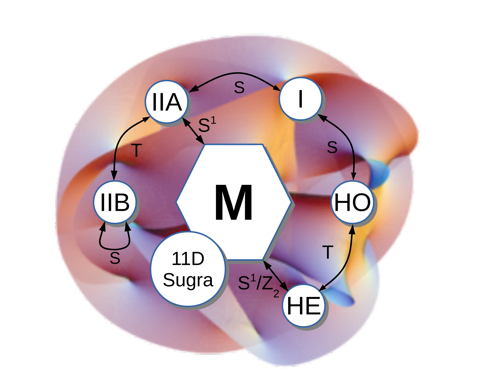
Twenty years ago it was realised that strings also imply branes [183], which are solitonic sub-dimensional objects in spatial dimensions to which strings may attach themselves, and indeed must do so for consistency in certain string theories. Indeed it is possible that the SM gauge group is restricted to one or more of these branes. Including such -branes, there are other types of string theory denoted as type I, IIA, and IIB which are related by a complicated web of dualities, as depicted in Fig.20, where theory is supposed to be the Mother of all these string theories, whose low energy limit is 11-d supergravity. However a generic problem with -brane models is how to achieve unification, for example based on , and at the same time a renormalisable top quark Yukawa coupling originating from . The issue is that this term is usually forbidden by type symmetries arising from -brane models.
One way round this, which has attracted considerable interest over the recent years, are the F theory models based on type IIB string theory, but compactified on Calabi-Yao complex fourfold manifolds [184]. This can be thought of as an elliptic fibration over the base manifold , as shown in Fig. 21. Pinch points in the two-tori correspond to singularities in the base manifold where branes can intersect, with gauge fields such as living on the branes and matter fields at the intersection between branes (for a review see e.g. [185]). In Fig. 21, the group lives on the brane, while Yukawa couplings correspond to the intersection of matter curves. Interestingly exceptional groups such as can be supported on the branes (not just ) allowing Yukawa couplings to arise from the triple intersection of three fundamental multiplets [186].
The brane in Fig. 21 can also support an gauge group, denoted as , which is different from the group lives on the brane. The full gauge group is then , which is supposed to emerge from an point of enhancement [184]. however the gauge group is broken by fluxes which live on the branes, analogous to magnetic fields in the extra dimensions. For example, may be broken to the SM gauge group by hypercharge flux, where the mechanism naturally allows for doublet-triplet splitting.
The most common assumption is that is also broken to . The four groups are usually identified by so called “monodromy action” down to a smaller symmetry , where . The surviving group may be used as a family symmetry group, which controls the number of copies of each chiral SM multiplet. It may be further broken by additional singlet fields, which play the role of flavon fields, subject to the rules of F-theory, and such flavons may then appear in Yukawa operators from which the Yukawa matrices may be constructed [186].
It was conjectured in [187], that instead of being broken to the Abelian subgroup , it might instead be broken to the discrete non-Abelian subgroup , or one of its discrete subgroups , , , which might be identified as a family symmetry group. This possibility was studied in detail in [188], where models were constructed along these lines. However this conjecture is far from being established, and it a matter of debate whether or not such non-Abelian discrete family groups can emerge from F-theory.

It is worth to mention some recent developments in M theory compactified on manifiold. The motivation for such an approach is that M theory is at the centre of the web of dualities in Fig. 20, and is regarded by many as the most fundamental of all string theories. The phenomenological interest in compactification is in formulating a consistent , which is broken to the SM gauge group by Wilson line breaking which includes a natural mechanism for doublet-triplet splitting. The phenomenological consequences of such an approach have been discussed in the review article in [189], which contains many original references.
The approach has been extended to [190]. The Wilson line breaking mechanism preserves the rank of the gauge group, so that it can break via , down to the SM gauge group, but it can never break the gauge group. Furthermore, it was shown that the doublet-triplet splitting mechanism when applied to does not work in the same way as for , and results in extra vector-like states at roughly the TeV scale. The spectrum of extra vector-like states have the quantum numbers of a complete extra superfield representations of , although the GUT group is broken of course, and also the extra matter arises from different high energy and states [190].
The importance of for this review is of course that neutrino masses then become inevitable when it is broken to the SM gauge group. However, neutrino masses can only arise once the gauge group is broken, and this can only occur at the field theory level, since Wilson lines cannot reduce rank as mentioned above. The breaking of can be acheived through the VEVs of the RH sneutrino components of the , and neutrino masses then can arise via the operator . However the origin of neutrino mass is more complicated than this, since R-parity breaking is a generic consequence of the M theory approach, and the neutrino mass matrix for a single physical neutrino mass turns out to be an eleven by eleven matrix! We only remark here that a phenomenologically acceptable neutrino mass can emerge from this framework with both the type I seesaw mechanism and R-parity violation contributing to neutrino mass [190].
7 Conclusion
This concludes our review of Unified Models of Neutrinos, Flavour and violation. We have come a long way, starting from neutrino experiments and ending up with string theory. In the Introduction, we recalled the breathtaking advances in neutrino physics from 1998 onwards, then we summarised what is known and what remains to be learned from neutrino experiments, and why this means that we must go beyond the SM. After surveying the alternative mechanisms for the origin of neutrino mass, we emphasised the biggest impact of neutrino physics, namely on the flavour problem, then summarised the theoretical model building attempts to understand lepton mixing angles, which have had mixed success so far, leaving the present state of neutrino model building in its present chaotic state. Moving forwards, we have identified four pillars on which we advocate future models should be constructed, namely: predictivity, minimality, robustness and unification.
We first gave an up to date discussion of the latest global fits on lepton mixing parameters in which we saw that recent data from neutrino experiments gives intriguing hints on the pattern of neutrino masses, lepton mixing angles and the violating phase. Present data (slightly) prefers a normal ordered (NO) neutrino mass pattern, with a CP phase , and (more significantly) non-maximal atmospheric mixing. Global fits for the NO case yield lepton mixing angle one sigma ranges: , , . Cosmology and large scale structure further provide a limit on the sum of neutrino masses to be below about eV, favouring hierarchical neutrino masses over quasi-degenerate masses.
We then turned to the first pillar of any model: predictivity. Without this, there can be no discrimination between models based on experiment, and therefore no lasting progress. We should not be embarrassed as theorists that our models are excluded by experiment, since this represents progress; we should be much more concerned if our models do not make predictions and so cannot be excluded! In this spirit, we reviewed simple patterns of lepton mixing such as bimaximal, golden ratio and tri-bimaximal, which are not viable by themselves but may be combined with charged lepton corrections leading to solar mixing sum rules, or the structures may be partly preserved as in trimaximal lepton mixing leading to atmospheric mixing rules. Such sum rules are realistic targets for future experiments. Indeed it seems that the mixing sum rule is under severe tension, but the sum rule survives.
The second pillar of any model, minimality, was then rigorously applied. Casting aside a wealth of viable models of neutrinos, some of which were reviewed in the Introduction, we have mainly focussed on the most minimal origin of neutrino mass based on the elegant type I seesaw mechanism, including the one and two RH neutrino (RHN) models, the sequential dominance of three RH neutrinos, constrained sequential dominance and the highly predictive littlest seesaw (LS) models, which includes the mixing sum rules amongst its predictions. We discussed the impact of future precision oscillation experiments on the LS models, which shows that the planned experiments are quite capable of excluding these models. If they survive, then one must take such models seriously. If they are excluded then perhaps other models will emerge. In this way, progress towards understanding the flavour puzzle can be made.
The third pillar on which any model should be based is that of robustness, meaning that any model should not be ad hoc, but should have some theory behind it, or at least a symmetry. After a brief review of finite group theory, we identified the Klein symmetry relevant for the Majorana neutrino mass matrix, and how this may be embedded into a non-Abelian family symmetry spontaneously broken by flavons. We then described semi-direct models where only half the Klein symmetry is preserved in the neutrino sector, and discussed the LS model as an example. We then turned to spontaneous violation, including invariants and the consistency condition, before turning to the idea of residual , which allows the phases to be predicted.
Finally we turned to the fourth and final pillar which we advovate for models of flavour, namely that of unification. Although seemingly rather esoteric, it has a solid motivation in the history of physics going back to Maxwell’s electromagnetism. It also has a practical motivation, in that it necessarily brings in the quark sector into the same framework as the lepton sector, so that any unified theory of leptons will also be a theory of quarks as well. This is important, since any resolution to the flavour problem must include both quarks and leptons. After an introductions to GUTs, we discussed models which combine family symmetry with GUTs, the so called flavoured GUTs, limiting ourselves to a table of models in the literature, together with one example to illustrate the method. We finished off with some brief speculations about the possible string theory origin of such theories.
It is worth assessing where we stand in our quest towards a model of a unified model of neutrinos, flavour and violation, based on the four pillars of predictivity, minimality, robustness and unification. At this moment in time, the Littlest Seesaw model has emerged as a possible candidate which seems to satisfy all four requirements. Indeed, all of the examples discusssed in this review involve the Littlest Seesaw as a common thread which spans all four pillars. The reason for doing this is to show how any candidate theory should rest on these four principles. We could have chosen some other model to demonstrate this, and it really does not matter which: we chose the Littlest Seesaw since it provides a convenient example which highlights all four aspects of model building applied in a coherent way across all of the desiderata. Let us therefore briefly give a critique of the Littlest Seesaw model in all four categories.
The Littlest Seesaw is certainly predictive, with the neutrino masses and PMNS matrix fixed by two parameters, but on the other hand it is easy to rule it out by say the observation of an inverted ordering, or a definitive observation of non-maximal atmospheric mixing in future experiments. The Littlest Seesaw is definitely minimal, involving just two RH neutrinos in the type I seesaw mechanism, but we need to explain why in a particular basis the two right-handed neutrino mass matrix and the charged lepton mass matrix are diagonal, and why in this basis the Dirac mass matrix has the CSD(3) form. The Littlest Seesaw may be robust, in the sense that the required vacuum alignments for type B at least may arise from symmetry realised in a semi-direct way with residual in the charged lepton sector and in the neutrino sector, but on the other hand the actual details of dynamical vacuum alignment (not discussed here) are still quite complicated. The Littlest Seesaw can be incorporated into a unified model based on , but in practice we saw that such models are still rather complicated, involving rather large additional discrete symmetries as well as large numbers of flavon and messenger fields. Fortunately the additional parameters which appear in the ultraviolet do not seem to be relevant for the low energy predictions of the model, but this does not alter the fact that these models are complicated. Perhaps the ultraviolet completion of these models in the framework of string theory could eventually lead to a simpler theory, at least in principle?
In conclusion, the discovery of neutrino mass and mixing continues to offer tantalising clues that may help to unravel the mystery of fermion flavour, mass, mixing and violation. Although neutrino model building appears presently to be in disarray, the emerging experimental consensus on some of the open questions in neutrino physics such as the ordering, scale and nature of neutrino mass and the latest hints on the lepton mixing angles and phase, will serve to shed light on the correct model building path. By constructing models based on the four pillars of predictivity, minimality, robustness and unification, it may be possible for some young researcher reading this to eventually realise Feynman’s dream of understanding flavour.
The author acknowledges the STFC Consolidated Grant ST/L000296/1 and the European Union’s Horizon 2020 Research and Innovation programme under Marie Skłodowska-Curie grant agreements Elusives ITN No. 674896 and InvisiblesPlus RISE No. 690575.
Appendix
Appendix A and group theory
The Kronecker products of the groups are basis independent but the values of the Clebsch-Gordan coefficients depend on the basis. We denote the Kronecker products and Clebsch-Gordan coefficients of in the basis of Eq.88 by the following (where counts the number of primes which appear, e.g. has primes):
The Clebsch-Gordan coefficients can be obtained from these expressions by simply dropping all primes and identifying the components of the doublet as the and representations of . We thus find the non-trivial products, explicitly,
Although the table in Eq.88 shows the diagonal basis of , it is sometimes convenient to work in diagonal basis in which all matrices are real in the triplet representation [27],
| (154) |
From these generators one may obtain all 12 real matrix group elements after multiplying these two matrices together in all possible ways [27]. Note that although the basis in Eq.154 differs from Eq.88, in both bases is traceless since and is said to have zero character in all bases, while has a character (or trace) of in all bases. In the basis of Eq.154 one has the following Clebsch rules for the multiplication of two triplets, , with
| (155) |
where and are the two triplets and . These differ from the Clebsch rules in the diagonal (but complex) basis given earlier, showing that, although the Kronecker product decomposition is valid in all bases, the Clebsch rules are basis dependent.
References
- [1]
Special Issue on
“Neutrino Oscillations: Celebrating the Nobel Prize in Physics 2015”
Edited by Tommy Ohlsson,
Nucl. Phys. B 908 (2016) Pages 1-466 (July 2016),
http://www.sciencedirect.com/science/journal/05503213/908/supp/C. - [2]
Neutrino experiments can be found at,
https://en.wikipedia.org/wiki/List_of_neutrino_experiments - [3] Neutrino 2016, The XXVII International Conference on Neutrino Physics and Astrophysics, London 4-9 July, 2016, http://neutrino2016.iopconfs.org/programme
- [4] S. Weinberg, Phys. Rev. D 22 (1980) 1694.
- [5] P. Minkowski, Phys. Lett. B 67 (1977) 421; T. Yanagida in Proc. of the Workshop on Unified Theory and Baryon Number of the Universe, KEK, Japan (1979); M. Gell-Mann, P. Ramond and R. Slansky in Sanibel Talk, CALT-68-709, Feb 1979, and in Supergravity, North Holland, Amsterdam (1979); S. L. Glashow, Cargese Lectures (1979); R. N. Mohapatra and G. Senjanovic, Phys. Rev. Lett. 44 (1980) 912.
- [6] M. Magg and C. Wetterich, Phys. Lett. B 94 (1980) 61; J. Schechter and J. W. F. Valle, Phys. Rev. D 22 (1980) 2227; G. Lazarides, Q. Shafi and C. Wetterich, Nucl. Phys. B 181 (1981) 287; R. N. Mohapatra and G. Senjanovic, Phys. Rev. D 23 (1981) 165; C. Wetterich, Nucl. Phys. B 187 (1981) 343.
- [7] R. Foot, H. Lew, X. G. He and G. C. Joshi, Z. Phys. C 44 (1989) 441.
- [8] S. F. King and T. Yanagida, Prog. Theor. Phys. 114 (2006) 1035 [hep-ph/0411030]. S. Morisi and J. W. F. Valle, Fortsch. Phys. 61 (2013) 466 [arXiv:1206.6678 [hep-ph]]; R. N. Mohapatra and A. Perez-Lorenzana, Phys. Rev. D 66 (2002) 035005 [hep-ph/0205347]; R. N. Mohapatra and A. Perez-Lorenzana, Phys. Rev. D 67 (2003) 075015 [hep-ph/0212254]; C. H. Lee, P. S. Bhupal Dev and R. N. Mohapatra, Phys. Rev. D 88 (2013) no.9, 093010 [arXiv:1309.0774 [hep-ph]]; R. N. Mohapatra, Nucl. Phys. B 908 (2016) 423; S. M. Boucenna, S. Morisi and J. W. F. Valle, Adv. High Energy Phys. 2014 (2014) 831598 [arXiv:1404.3751 [hep-ph]]; L. Basso, A. Belyaev, S. Moretti and C. H. Shepherd-Themistocleous, Phys. Rev. D 80 (2009) 055030 [arXiv:0812.4313 [hep-ph]].
- [9] L. J. Hall and M. Suzuki, Nucl. Phys. B 231 (1984) 419; Y. Grossman and H. E. Haber, Phys. Rev. Lett. 78 (1997) 3438 [hep-ph/9702421]; M. A. Diaz, J. C. Romao and J. W. F. Valle, Nucl. Phys. B 524 (1998) 23 [hep-ph/9706315]; H. K. Dreiner, in Kane, G.L. (ed.) Perspectives on supersymmetry II 565 [hep-ph/9707435]; M. A. Diaz, in Jerusalem 1997, High energy physics 895 [hep-ph/9712213]; M. Drees, S. Pakvasa, X. Tata and T. ter Veldhuis, Phys. Rev. D 57 (1998) 5335 [hep-ph/9712392]; A. Faessler, S. Kovalenko and F. Simkovic, Phys. Rev. D 58 (1998) 055004 [hep-ph/9712535]; E. J. Chun, Phys. Lett. B 454 (1999) 304 [hep-ph/9901220]; A. Abada and M. Losada, Nucl. Phys. B 585 (2000) 45 [hep-ph/9908352]; M. Hirsch, M. A. Diaz, W. Porod, J. C. Romao and J. W. F. Valle, Phys. Rev. D 62 (2000) 113008 [Erratum-ibid. D 65 (2002) 119901] [hep-ph/0004115]; F. De Campos, M. A. Diaz, O. J. P. Eboli, M. B. Magro and P. G. Mercadante, Nucl. Phys. B 623 (2002) 47 [hep-ph/0110049]; M. A. Diaz, M. Hirsch, W. Porod, J. C. Romao and J. W. F. Valle, Phys. Rev. D 68 (2003) 013009 [Erratum-ibid. D 71 (2005) 059904] [hep-ph/0302021]; M. Hirsch and W. Porod, Phys. Rev. D 68 (2003) 115007 [hep-ph/0307364]; R. Barbier, C. Berat, M. Besancon, M. Chemtob, A. Deandrea, E. Dudas, P. Fayet and S. Lavignac et al., Phys. Rept. 420 (2005) 1 [hep-ph/0406039]; F. de Campos, M. A. Diaz, O. J. P. Eboli, R. A. Lineros, M. B. Magro and P. G. Mercadante, Phys. Rev. D 71 (2005) 055008 [hep-ph/0409043]; D. Aristizabal Sierra, M. Hirsch and W. Porod, JHEP 0509 (2005) 033 [hep-ph/0409241]; E. J. Chun and S. C. Park, JHEP 0501 (2005) 009 [hep-ph/0410242]; M. A. Diaz, C. Mora and A. R. Zerwekh, Eur. Phys. J. C 44 (2005) 277 [hep-ph/0410285]; A. Dedes, S. Rimmer and J. Rosiek, JHEP 0608 (2006) 005 [hep-ph/0603225]; H. K. Dreiner, C. Luhn, H. Murayama and M. Thormeier, Nucl. Phys. B 774 (2007) 127 [hep-ph/0610026]; B. C. Allanach and C. H. Kom, JHEP 0804 (2008) 081 [arXiv:0712.0852]; H. K. Dreiner, M. Hanussek and S. Grab, Phys. Rev. D 82 (2010) 055027 [arXiv:1005.3309]; H. K. Dreiner, M. Hanussek, J. -S. Kim and C. H. Kom, Phys. Rev. D 84 (2011) 113005 [arXiv:1106.4338]; B. C. Allanach, C. H. Kom and M. Hanussek, Comput. Phys. Commun. 183 (2012) 785 [arXiv:1109.3735]; F. Bazzocchi, S. Morisi, E. Peinado, J. W. F. Valle and A. Vicente, JHEP 1301 (2013) 033 [arXiv:1202.1529]; H. K. Dreiner, M. Hanussek and C. Luhn, Phys. Rev. D 86 (2012) 055012 [arXiv:1206.6305]; E. Peinado and A. Vicente, Phys. Rev. D 86 (2012) 093024 [arXiv:1207.6641].
- [10] A. Zee, Phys. Lett. B 93 (1980) 389 [Erratum-ibid. B 95 (1980) 461]; T. P. Cheng and L. -F. Li, Phys. Rev. D 22 (1980) 2860; S. T. Petcov, Phys. Lett. B 115 (1982) 401; K. S. Babu, Phys. Lett. B 203 (1988) 132; N. G. Deshpande, J. F. Gunion, B. Kayser and F. I. Olness, Phys. Rev. D 44 (1991) 837; C. Jarlskog, M. Matsuda, S. Skadhauge and M. Tanimoto, Phys. Lett. B 449 (1999) 240 [hep-ph/9812282]; Y. Koide and A. Ghosal, Phys. Rev. D 63 (2001) 037301 [hep-ph/0008129]; K. R. S. Balaji, W. Grimus and T. Schwetz, Phys. Lett. B 508 (2001) 301 [hep-ph/0104035]; T. Kitabayashi and M. Yasue, Phys. Lett. B 524 (2002) 308 [hep-ph/0110303]; T. Kitabayashi and M. Yasue, Int. J. Mod. Phys. A 17 (2002) 2519 [hep-ph/0112287]; E. J. Chun, K. Y. Lee and S. C. Park, Phys. Lett. B 566 (2003) 142 [hep-ph/0304069]; X. -G. He, Eur. Phys. J. C 34 (2004) 371 [hep-ph/0307172]; V. Cirigliano, A. Kurylov, M. J. Ramsey-Musolf and P. Vogel, Phys. Rev. D 70 (2004) 075007 [hep-ph/0404233]; A. G. Akeroyd and M. Aoki, Phys. Rev. D 72 (2005) 035011 [hep-ph/0506176]; R. Bouchand and A. Merle, JHEP 1207 (2012) 084 [arXiv:1205.0008]; A. Pilaftsis, Z. Phys. C 55 (1992) 275 [hep-ph/9901206]; P. S. B. Dev and A. Pilaftsis, Phys. Rev. D 86 (2012) 113001 [arXiv:1209.4051 [hep-ph]]; E. Ma, A. Natale and A. Rashed, Int. J. Mod. Phys. A 27 (2012) 1250134 [arXiv:1206.1570]; S. F. King, A. Merle and L. Panizzi, JHEP 1411 (2014) 124 [arXiv:1406.4137 [hep-ph]]; T. Geib, S. F. King, A. Merle, J. M. No and L. Panizzi, Phys. Rev. D 93 (2016) no.7, 073007 [arXiv:1512.04391 [hep-ph]].
- [11] N. Arkani-Hamed, S. Dimopoulos and G. R. Dvali, Phys. Lett. B 429 (1998) 263 [hep-ph/9803315]; K. R. Dienes, E. Dudas and T. Gherghetta, Nucl. Phys. B 557 (1999) 25 [hep-ph/9811428]; N. Arkani-Hamed, S. Dimopoulos, G. R. Dvali and J. March-Russell, Phys. Rev. D 65 (2002) 024032 [hep-ph/9811448]; A. E. Faraggi and M. Pospelov, Phys. Lett. B 458 (1999) 237 [hep-ph/9901299]; G. R. Dvali and A. Y. .Smirnov, Nucl. Phys. B 563 (1999) 63 [hep-ph/9904211]; R. N. Mohapatra, S. Nandi and A. Perez-Lorenzana, Phys. Lett. B 466 (1999) 115 [hep-ph/9907520]; R. Barbieri, P. Creminelli and A. Strumia, Nucl. Phys. B 585 (2000) 28 [hep-ph/0002199].
- [12] R. N. Mohapatra and J. W. Valle, Phys. Rev. D 34 (1986) 1642; A. E. Faraggi and E. Halyo, Phys. Lett. B 307 (1993) 311 [hep-th/9303060]; N. Haba, C. Hattori, M. Matsuda, T. Matsuoka and D. Mochinaga, Phys. Lett. B 337 (1994) 63 [hep-ph/9311298]; N. Haba, C. Hattori, M. Matsuda, T. Matsuoka and D. Mochinaga, Prog. Theor. Phys. 92 (1994) 153 [hep-ph/9401332]; G. Cleaver, M. Cvetic, J. R. Espinosa, L. L. Everett and P. Langacker, Phys. Rev. D 57 (1998) 2701 [hep-ph/9705391]; J. R. Ellis, G. K. Leontaris, S. Lola and D. V. Nanopoulos, Phys. Lett. B 425 (1998) 86 [hep-ph/9711476]; P. Langacker, Phys. Rev. D 58 (1998) 093017 [hep-ph/9805281]; J. R. Ellis, G. K. Leontaris, S. Lola and D. V. Nanopoulos, Eur. Phys. J. C 9 (1999) 389 [hep-ph/9808251]; L. E. Ibanez, C. Munoz and S. Rigolin, Nucl. Phys. B 553 (1999) 43 [hep-ph/9812397]; C. Coriano and A. E. Faraggi, Phys. Lett. B 581 (2004) 99 [hep-ph/0306186]; J. E. Kim, Phys. Lett. B 591 (2004) 119 [hep-ph/0403196]; J. Giedt, G. L. Kane, P. Langacker and B. D. Nelson, Phys. Rev. D 71 (2005) 115013 [hep-th/0502032]; S. Antusch, O. J. Eyton-Williams and S. F. King, JHEP 0508 (2005) 103 [hep-ph/0505140]; P. Langacker and B. D. Nelson, Phys. Rev. D 72 (2005) 053013 [hep-ph/0507063].
- [13] A. Bandyopadhyay et al. [ISS Physics Working Group Collaboration], Rept. Prog. Phys. 72 (2009) 106201 [arXiv:0710.4947]; S. Morisi and J. W. F. Valle, Fortsch. Phys. 61 (2013) 466 doi:10.1002/prop.201200125 [arXiv:1206.6678 [hep-ph]]; D. Aristizabal Sierra, Acta Phys. Polon. B 46 (2015) no.11, 2311 doi:10.5506/APhysPolB.46.2311 [arXiv:1510.03762 [hep-ph]]; G. Senjanovic and V. Tello, PoS PLANCK 2015 (2016) 141.
- [14] “QED - the strange theory of light and matter” (Penguin Press Science), R. P. Feynman.
- [15] G. Altarelli and F. Feruglio, Phys. Rept. 320 (1999) 295.
- [16] S. F. King, Rept. Prog. Phys. 67 (2004) 107 [hep-ph/0310204].
- [17] R. N. Mohapatra and A. Y. Smirnov, Ann. Rev. Nucl. Part. Sci. 56 (2006) 569 [hep-ph/0603118].
- [18] G. Altarelli and F. Feruglio, Rev. Mod. Phys. 82, 2701 (2010) [arXiv:1002.0211 [hep-ph]].
- [19] H. Ishimori, T. Kobayashi, H. Ohki, Y. Shimizu, H. Okada and M. Tanimoto, Prog. Theor. Phys. Suppl. 183, 1 (2010) [arXiv:1003.3552 [hep-th]]; H. Ishimori, T. Kobayashi, H. Ohki, H. Okada, Y. Shimizu and M. Tanimoto, Lect. Notes Phys. 858, 1 (2012); H. Ishimori, T. Kobayashi, Y. Shimizu, H. Ohki, H. Okada and M. Tanimoto, Fortsch. Phys. 61, 441 (2013).
- [20] S. F. King and C. Luhn, Rept. Prog. Phys. 76 (2013) 056201 [arXiv:1301.1340].
- [21] S. F. King, A. Merle, S. Morisi, Y. Shimizu and M. Tanimoto, New J. Phys. 16 (2014) 045018 [arXiv:1402.4271].
- [22] S. F. King, J. Phys. G 42 (2015) 123001 [arXiv:1510.02091 [hep-ph]].
- [23] S. F. King, Phys. Lett. B 439 (1998) 350 [hep-ph/9806440]; S. F. King, Nucl. Phys. B 562 (1999) 57 [hep-ph/9904210].
- [24] S. F. King, Nucl. Phys. B 576 (2000) 85 [hep-ph/9912492].
- [25] S. F. King, JHEP 0209 (2002) 011 [hep-ph/0204360]; S. F. King, Phys. Rev. D 67 (2003) 113010 [hep-ph/0211228].
- [26] S. F. King and G. G. Ross, Phys. Lett. B 520 (2001) 243 [hep-ph/0108112]; S. F. King and G. G. Ross, Phys. Lett. B 574 (2003) 239 [hep-ph/0307190].
- [27] E. Ma and G. Rajasekaran, Phys. Rev. D 64 (2001) 113012 [hep-ph/0106291].
- [28] G. Altarelli and F. Feruglio, Nucl. Phys. B 720 (2005) 64 [hep-ph/0504165]; G. Altarelli and F. Feruglio, Nucl. Phys. B 741 (2006) 215 [hep-ph/0512103]; I. de Medeiros Varzielas, S. F. King and G. G. Ross, Phys. Lett. B 644 (2007) 153 [hep-ph/0512313]; I. de Medeiros Varzielas, S. F. King and G. G. Ross, Phys. Lett. B 648 (2007) 201 [hep-ph/0607045].
- [29] S. Zhou, Phys. Lett. B 704 (2011) 291 [arXiv:1106.4808]; S. Dev, R. R. Gautam and L. Singh, Phys. Lett. B 708 (2012) 284 [arXiv:1201.3755]; D. Meloni, S. Morisi and E. Peinado, Eur. Phys. J. C 72 (2012) 2160 [arXiv:1203.2535]; D. Meloni, JHEP 1205 (2012) 124 [arXiv:1203.3126]; A. G. Dias, A. C. B. Machado and C. C. Nishi, Phys. Rev. D 86 (2012) 093005 [arXiv:1206.6362].
- [30] X. -G. He and A. Zee, Phys. Lett. B 645 (2007) 427 [hep-ph/0607163]; B. Adhikary and A. Ghosal, Phys. Rev. D 75 (2007) 073020 [hep-ph/0609193]; M. Hirsch, A. S. Joshipura, S. Kaneko and J. W. F. Valle, Phys. Rev. Lett. 99 (2007) 151802 [hep-ph/0703046]; Y. Lin, Nucl. Phys. B 824 (2010) 95 [arXiv:0905.3534]; S. Morisi and E. Peinado, Phys. Rev. D 80 (2009) 113011 [arXiv:0910.4389]; Y. H. Ahn and C. -S. Chen, Phys. Rev. D 81 (2010) 105013 [arXiv:1001.2869]; Y. H. Ahn, H. -Y. Cheng and S. Oh, Phys. Rev. D 83 (2011) 076012 [arXiv:1102.0879]; I. K. Cooper, S. F. King and C. Luhn, Nucl. Phys. B 859 (2012) 159 [arXiv:1110.5676]; S. Gupta, A. S. Joshipura and K. M. Patel, Phys. Rev. D 85 (2012) 031903 [arXiv:1112.6113]; K. Siyeon, Eur. Phys. J. 72 (2012) 2081 [arXiv:1203.1593]; G. C. Branco, R. Gonzalez Felipe, F. R. Joaquim and H. Serodio, Phys. Rev. D 86 (2012) 076008 [arXiv:1203.2646]; Y. H. Ahn and S. K. Kang, Phys. Rev. D 86 (2012) 093003 [arXiv:1203.4185]; G. Altarelli, F. Feruglio and L. Merlo, Fortsch. Phys. 61 (2013) 507 [arXiv:1205.5133 [hep-ph]]; W. Rodejohann and H. Zhang, Phys. Rev. D 86 (2012) 093008 [arXiv:1207.1225]; Y. BenTov, X. G. He and A. Zee, JHEP 1212 (2012) 093 doi:10.1007/JHEP12(2012)093 [arXiv:1208.1062 [hep-ph]]; M. C. Chen, J. Huang, J. M. O’Bryan, A. M. Wijangco and F. Yu, JHEP 1302 (2013) 021 [arXiv:1210.6982 [hep-ph]]; M. Holthausen, M. Lindner and M. A. Schmidt, Phys. Rev. D 87 (2013) no.3, 033006 [arXiv:1211.5143 [hep-ph]]. I. d. M. Varzielas and D. Pidt, UV completions of flavour models and large , arXiv:1211.5370; S. Morisi, D. V. Forero, J. C. Romo and J. W. F. Valle, Phys. Rev. D 88 (2013) no.1, 016003 [arXiv:1305.6774 [hep-ph]]; S. Morisi, M. Nebot, K. M. Patel, E. Peinado and J. W. F. Valle, Phys. Rev. D 88 (2013) 036001 [arXiv:1303.4394 [hep-ph]]; S. F. King, S. Morisi, E. Peinado and J. W. F. Valle, Phys. Lett. B 724 (2013) 68 [arXiv:1301.7065 [hep-ph]]; M. S. Boucenna, M. Hirsch, S. Morisi, E. Peinado, M. Taoso and J. W. F. Valle, JHEP 1105 (2011) 037 [arXiv:1101.2874 [hep-ph]]; M. Hirsch, S. Morisi and J. W. F. Valle, Phys. Lett. B 679 (2009) 454 [arXiv:0905.3056 [hep-ph]].
- [31] C. Hagedorn, M. Lindner and R. N. Mohapatra, JHEP 0606 (2006) 042 [hep-ph/0602244]; H. Ishimori, Y. Shimizu, M. Tanimoto and A. Watanabe, Phys. Rev. D 83 (2011) 033004 [arXiv:1010.3805]; H. Ishimori and T. Kobayashi, JHEP 1110 (2011) 082 [arXiv:1106.3604]; S. Morisi, K. M. Patel and E. Peinado, Phys. Rev. D 84 (2011) 053002 [arXiv:1107.0696]; H. -J. He and X. -J. Xu, Phys. Rev. D 86 (2012) 111301 [arXiv:1203.2908]; F. Bazzocchi and L. Merlo, arXiv:1205.5135; R. N. Mohapatra and C. C. Nishi, Phys. Rev. D 86 (2012) 073007 [arXiv:1208.2875]; R. Krishnan, P. F. Harrison and W. G. Scott, JHEP 1304 (2013) 087 [arXiv:1211.2000 [hep-ph]]; R. Krishnan, J. Phys. Conf. Ser. 447 (2013) 012043 [arXiv:1211.3364 [hep-ph]]; F. Feruglio, C. Hagedorn and R. Ziegler, JHEP 1307 (2013) 027 [arXiv:1211.5560 [hep-ph]].
- [32] L. J. Hall, H. Murayama and N. Weiner, Phys. Rev. Lett. 84 (2000) 2572 [hep-ph/9911341]; M. Hirsch and S. F. King, Phys. Lett. B 516 (2001) 103 [hep-ph/0102103]; G. Altarelli, F. Feruglio and I. Masina, JHEP 0301 (2003) 035 [hep-ph/0210342]; A. de Gouvea and H. Murayama, Phys. Lett. B 573 (2003) 94 [hep-ph/0301050]; A. de Gouvea and H. Murayama, Phys. Lett. B 747 (2015) 479 [arXiv:1204.1249 [hep-ph]].
- [33] S. F. King, Phys. Lett. B 675 (2009) 347 [arXiv:0903.3199 [hep-ph]].
- [34] S. F. King and C. Luhn, JHEP 1203 (2012) 036 [arXiv:1112.1959 [hep-ph]].
- [35] P. A. R. Ade et al. [Planck Collaboration], Astron. Astrophys. 594 (2016) A13 [arXiv:1502.01589 [astro-ph.CO]].
- [36] S. Hannestad, arXiv:1605.03829 [astro-ph.CO].
- [37] A. Ghalsasi and A. E. Nelson, Phys. Rev. D 90 (2014) no.4, 045002 [arXiv:1405.0711 [hep-ph]].
- [38] M. C. Gonzalez-Garcia, M. Maltoni and T. Schwetz, JHEP 1411 (2014) 052 [arXiv:1409.5439 [hep-ph]]; I. Esteban, M. C. Gonzalez-Garcia, M. Maltoni, I. Martinez-Soler and T. Schwetz, arXiv:1611.01514 [hep-ph]; NuFIT 3.0 (2016), http://www.nu-fit.org.
- [39] F. Capozzi, G. L. Fogli, E. Lisi, A. Marrone, D. Montanino and A. Palazzo, Phys. Rev. D 89 (2014) 093018 [arXiv:1312.2878]; latest update: F. Capozzi, E. Lisi, A. Marrone, D. Montanino and A. Palazzo, Proceedings of Neutrino 2016, The XXVII International Conference on Neutrino Physics and Astrophysics, London 4-9 July, 2016 (talk by Antonio Marrone).
- [40] D. V. Forero, M. Tortola and J. W. F. Valle, Phys. Rev. D 90 (2014) 9, 093006 [arXiv:1405.7540 [hep-ph]]; no further update currently available.
- [41] C. Patrignani et al. (Particle Data Group), Chin. Phys. C 40, 100001 (2016) 1.
- [42] H. Minakata and A. Y. Smirnov, Phys. Rev. D 70 (2004) 073009 doi:10.1103/PhysRevD.70.073009 [hep-ph/0405088]; S. F. King, Phys. Lett. B 718 (2012) 136 [arXiv:1205.0506 [hep-ph]]; D. V. Ahluwalia, ISRN High Energy Phys. 2012 (2012) 954272 [arXiv:1206.4779 [hep-ph]]; S. Antusch, C. Gross, V. Maurer and C. Sluka, Nucl. Phys. B 877 (2013) 772 doi:10.1016/j.nuclphysb.2013.11.003 [arXiv:1305.6612 [hep-ph]].
- [43] S. F. King, A. Merle and A. J. Stuart, JHEP 1312 (2013) 005 [arXiv:1307.2901 [hep-ph]].
- [44] V. D. Barger, S. Pakvasa, T. J. Weiler and K. Whisnant, Phys. Lett. B 437 (1998) 107 [hep-ph/9806387]; S. Davidson and S. F. King, Phys. Lett. B 445 (1998) 191 [hep-ph/9808296].
- [45] A. Datta, F. S. Ling and P. Ramond, Nucl. Phys. B 671 (2003) 383 [hep-ph/0306002]; L. L. Everett and A. J. Stuart, Phys. Rev. D 79 (2009) 085005 [arXiv:0812.1057]; F. Feruglio and A. Paris, JHEP 1103 (2011) 101 [arXiv:1101.0393].
- [46] W. Rodejohann, Phys. Lett. B 671 (2009) 267 [arXiv:0810.5239 [hep-ph]]; A. Adulpravitchai, A. Blum and W. Rodejohann, New J. Phys. 11 (2009) 063026 [arXiv:0903.0531 [hep-ph]].
- [47] P. F. Harrison, D. H. Perkins and W. G. Scott, Phys. Lett. B 530 (2002) 167 [hep-ph/0202074]; Z. z. Xing, Phys. Lett. B 533 (2002) 85 [hep-ph/0204049].
- [48] S. F. King, Phys. Lett. B 659 (2008) 244 [arXiv:0710.0530 [hep-ph]].
- [49] S. Pakvasa, W. Rodejohann and T. J. Weiler, Phys. Rev. Lett. 100 (2008) 111801 [arXiv:0711.0052 [hep-ph]].
- [50] C. H. Albright and W. Rodejohann, Eur. Phys. J. C 62 (2009) 599 [arXiv:0812.0436 [hep-ph]]; C. H. Albright, A. Dueck and W. Rodejohann, Eur. Phys. J. C 70 (2010) 1099 [arXiv:1004.2798 [hep-ph]]; W. Grimus and L. Lavoura, JHEP 0809 (2008) 106 [arXiv:0809.0226 [hep-ph]]; Z. z. Xing and S. Zhou, Phys. Lett. B 653 (2007) 278 [hep-ph/0607302].
- [51] Y. Shimizu, M. Tanimoto and A. Watanabe, Prog. Theor. Phys. 126 (2011) 81 [arXiv:1105.2929]; S. F. King and C. Luhn, JHEP 1109 (2011) 042 [arXiv:1107.5332 [hep-ph]].
- [52] C. Luhn, Nucl. Phys. B 875 (2013) 80 [arXiv:1306.2358 [hep-ph]].
- [53] D. Hernandez and A. Y. Smirnov, Phys. Rev. D 86 (2012) 053014 [arXiv:1204.0445]; D. Hernandez and A. Y. Smirnov, Phys. Rev. D 87 (2013) 5, 053005 [arXiv:1212.2149].
- [54] P. Ballett, S. F. King, C. Luhn, S. Pascoli and M. A. Schmidt, Phys. Rev. D 89 (2014) 016016 [arXiv:1308.4314].
- [55] S. F. King, JHEP 0508 (2005) 105 [hep-ph/0506297].
- [56] I. Masina, Phys. Lett. B 633 (2006) 134 [hep-ph/0508031].
- [57] S. Antusch and S. F. King, Phys. Lett. B 631 (2005) 42 [hep-ph/0508044].
- [58] S. Antusch, P. Huber, S. F. King and T. Schwetz, JHEP 0704 (2007) 060 [hep-ph/0702286].
- [59] P. Ballett, S. F. King, C. Luhn, S. Pascoli and M. A. Schmidt, JHEP 1412 (2014) 122 [arXiv:1410.7573 [hep-ph]].
- [60] D. Marzocca, S. T. Petcov, A. Romanino and M. C. Sevilla, JHEP 1305 (2013) 073 [arXiv:1302.0423]; I. Girardi, S. T. Petcov and A. V. Titov, Nucl. Phys. B 894 (2015) 733 [arXiv:1410.8056 [hep-ph]]; S. T. Petcov, Nucl. Phys. B 892 (2015) 400 [arXiv:1405.6006 [hep-ph]]; J. Gehrlein, S. T. Petcov, M. Spinrath and A. V. Titov, JHEP 1611 (2016) 146 [arXiv:1608.08409 [hep-ph]]; I. Girardi, S. T. Petcov and A. V. Titov, Nucl. Phys. B 894 (2015) 733 [arXiv:1410.8056 [hep-ph]].
- [61] M. Drewes, PoS NUFACT 2014 (2015) 001 [arXiv:1502.06891 [hep-ph]];
- [62] P. H. Frampton, S. L. Glashow and T. Yanagida, Phys. Lett. B 548 (2002) 119 [hep-ph/0208157].
- [63] K. Harigaya, M. Ibe and T. T. Yanagida, Phys. Rev. D 86 (2012) 013002 [arXiv:1205.2198 [hep-ph]].
- [64] S. Antusch, S. F. King, C. Luhn and M. Spinrath, Nucl. Phys. B 856 (2012) 328 [arXiv:1108.4278].
- [65] S. F. King, JHEP 1307 (2013) 137 [arXiv:1304.6264].
- [66] S. F. King, Phys. Lett. B 724 (2013) 92 [arXiv:1305.4846].
- [67] S. F. King, JHEP 1401 (2014) 119 [arXiv:1311.3295 [hep-ph]].
- [68] S. F. King, JHEP 1408 (2014) 130 [arXiv:1406.7005 [hep-ph]].
- [69] F. Bjorkeroth and S. F. King, J. Phys. G 42 (2015) no.12, 125002 [arXiv:1412.6996 [hep-ph]].
- [70] F. Bjorkeroth, F. J. de Anda, I. de Medeiros Varzielas and S. F. King, JHEP 1510 (2015) 104 [arXiv:1505.05504 [hep-ph]].
- [71] S. F. King, JHEP 1602 (2016) 085 [arXiv:1512.07531 [hep-ph]].
- [72] S. F. King and C. Luhn, JHEP 1609 (2016) 023 [arXiv:1607.05276 [hep-ph]].
- [73] S. F. King, J. Zhang and S. Zhou, arXiv:1609.09402 [hep-ph].
- [74] P. Ballett, S. F. King, S. Pascoli, N. W. Prouse and T. Wang, arXiv:1612.01999 [hep-ph].
- [75] P. Ballett, S. F. King, S. Pascoli, N. W. Prouse and T. Wang, arXiv:1612.07275 [hep-ph].
- [76] T. Ohlsson and S. Zhou, Nature Commun. 5 (2014) 5153 [arXiv:1311.3846 [hep-ph]].
- [77] J. A. Escobar and C. Luhn, J. Math. Phys. 50 (2009) 013524 [arXiv:0809.0639 [hep-th]].
- [78] I. de Medeiros Varzielas, S. F. King and G. G. Ross, Neutrino tri-bimaximal mixing from a non-Abelian discrete family symmetry, Phys. Lett. B 648 (2007) 201 [hep-ph/0607045]; E. Ma, Neutrino mass matrix from symmetry, Mod. Phys. Lett. A 21 (2006) 1917 [hep-ph/0607056]; F. Bazzocchi and I. de Medeiros Varzielas, Tri-bimaximal mixing in viable family symmetry unified model with extended see-saw, Phys. Rev. D 79 (2009) 093001 [arXiv:0902.3250]; I. de Medeiros Varzielas and D. Emmanuel-Costa, Geometrical CP violation, Phys. Rev. D 84 (2011) 117901 [arXiv:1106.5477].
- [79] C. Luhn, S. Nasri and P. Ramond, J. Math. Phys. 48 (2007) 073501 [hep-th/0701188].
- [80] C. Luhn, S. Nasri and P. Ramond, J. Math. Phys. 48 (2007) 123519 [arXiv:0709.1447 [hep-th]]; S. F. King and C. Luhn, Nucl. Phys. B 820 (2009) 269 [arXiv:0905.1686 [hep-ph]]; S. F. King and C. Luhn, Nucl. Phys. B 832 (2010) 414 [arXiv:0912.1344 [hep-ph]].
- [81] C. Luhn, S. Nasri and P. Ramond, Phys. Lett. B 652 (2007) 27 [arXiv:0706.2341]; C. Hagedorn, M. A. Schmidt and A. Y. .Smirnov, Phys. Rev. D 79 (2009) 036002 [arXiv:0811.2955]; Q. -H. Cao, S. Khalil, E. Ma and H. Okada, Phys. Rev. Lett. 106 (2011) 131801 [arXiv:1009.5415].
- [82] C. Hagedorn, S. F. King and C. Luhn, JHEP 1006 (2010) 048 [arXiv:1003.4249].
- [83] S. F. King and C. Luhn, JHEP 0910 (2009) 093 [arXiv:0908.1897].
- [84] R. M. Fonseca and W. Grimus, JHEP 1409 (2014) 033 [arXiv:1405.3678 [hep-ph]].
- [85] M. Holthausen, K. S. Lim and M. Lindner, Phys. Lett. B 721, 61 (2013) [arXiv:1212.2411 [hep-ph]].
- [86] S. F. King, T. Neder and A. J. Stuart, Phys. Lett. B 726 (2013) 312 [arXiv:1305.3200 [hep-ph]].
- [87] S. Antusch, S. F. King, C. Luhn and M. Spinrath, Nucl. Phys. B 850 (2011) 477 [arXiv:1103.5930 [hep-ph]]. G. G. Ross, L. Velasco-Sevilla and O. Vives, Nucl. Phys. B 692 (2004) 50 [hep-ph/0401064]; S. Antusch, S. F. King and M. Malinsky, JHEP 0806 (2008) 068 [arXiv:0708.1282 [hep-ph]].
- [88] J. Bernabeu, G. C. Branco and M. Gronau, Phys. Lett. B 169, 243 (1986); C. Jarlskog, Phys. Rev. Lett. 55 (1985) 1039.
- [89] G. C. Branco, I. de Medeiros Varzielas and S. F. King, Phys. Rev. D 92 (2015) 036007 [arXiv:1502.03105 [hep-ph]]; G. C. Branco, I. de Medeiros Varzielas and S. F. King, Nucl. Phys. B 899 (2015) 14 [arXiv:1505.06165 [hep-ph]].
- [90] G. C. Branco, L. Lavoura and M. N. Rebelo, Phys. Lett. B 180, 264 (1986); G. C. Branco, M. N. Rebelo and J. I. Silva-Marcos, Phys. Rev. Lett. 82, 683 (1999) [hep-ph/9810328]; H. K. Dreiner, J. S. Kim, O. Lebedev and M. Thormeier, Phys. Rev. D 76, 015006 (2007) [hep-ph/0703074 [HEP-PH]].
- [91] M. Holthausen, M. Lindner and M. A. Schmidt, JHEP 1304, 122 (2013) [arXiv:1211.6953 [hep-ph]].
- [92] F. Feruglio, C. Hagedorn and R. Ziegler, JHEP 1307, 027 (2013) [arXiv:1211.5560 [hep-ph]]; G. -J. Ding, S. F. King, C. Luhn and A. J. Stuart, JHEP 1305, 084 (2013) [arXiv:1303.6180 [hep-ph]]; F. Feruglio, C. Hagedorn and R. Ziegler, Eur. Phys. J. C 74, 2753 (2014) [arXiv:1303.7178 [hep-ph]]; G. -J. Ding, S. F. King and A. J. Stuart, JHEP 1312 (2013) 006 [arXiv:1307.4212].
- [93] G. C. Branco, J. M. Gerard and W. Grimus, Phys. Lett. B 136 (1984) 383.
- [94] V. Keus, S. F. King, S. Moretti and K. Yagyu, arXiv:1510.04028.
- [95] A. Mendez and A. Pomarol, Phys. Lett. B 272 (1991) 313.
- [96] L. Lavoura and J. P. Silva, Phys. Rev. D 50 (1994) 4619 [hep-ph/9404276].
- [97] F. J. Botella and J. P. Silva, Phys. Rev. D 51 (1995) 3870 [hep-ph/9411288].
- [98] G. C. Branco, M. N. Rebelo and J. I. Silva-Marcos, Phys. Lett. B 614 (2005) 187 [hep-ph/0502118].
- [99] S. Davidson and H. E. Haber, Phys. Rev. D 72 (2005) 035004 Erratum: [Phys. Rev. D 72 (2005) 099902] [hep-ph/0504050].
- [100] J. F. Gunion and H. E. Haber, Phys. Rev. D 72 (2005) 095002 [hep-ph/0506227].
- [101] I. de Medeiros Varzielas, S. F. King, C. Luhn and T. Neder, Phys. Rev. D 94 (2016) no.5, 056007 doi:10.1103/PhysRevD.94.056007 [arXiv:1603.06942 [hep-ph]].
- [102] G. Ecker, W. Grimus and W. Konetschny, Nucl. Phys. B 191, 465 (1981). doi:10.1016/0550-3213(81)90309-6; G. Ecker, W. Grimus and H. Neufeld, Nucl. Phys. B 247, 70 (1984). doi:10.1016/0550-3213(84)90373-0; G. Ecker, W. Grimus and H. Neufeld, J. Phys. A 20, L807 (1987). doi:10.1088/0305-4470/20/12/010; H. Neufeld, W. Grimus and G. Ecker, Int. J. Mod. Phys. A 3, 603 (1988). doi:10.1142/S0217751X88000254
- [103] W. Grimus and M. N. Rebelo, Phys. Rept. 281, 239 (1997) doi:10.1016/S0370-1573(96)00030-0 [hep-ph/9506272].
- [104] P. F. Harrison and W. G. Scott, Phys. Lett. B 535, 163 (2002) doi:10.1016/S0370-2693(02)01753-7 [hep-ph/0203209]; P. F. Harrison and W. G. Scott, Phys. Lett. B 547, 219 (2002) doi:10.1016/S0370-2693(02)02772-7 [hep-ph/0210197]; P. F. Harrison and W. G. Scott, Phys. Lett. B 594, 324 (2004) doi:10.1016/j.physletb.2004.05.039 [hep-ph/0403278].
- [105] W. Grimus and L. Lavoura, Phys. Lett. B 579, 113 (2004) doi:10.1016/j.physletb.2003.10.075 [hep-ph/0305309]; W. Grimus and L. Lavoura, Fortsch. Phys. 61, 535 (2013) doi:10.1002/prop.201200118 [arXiv:1207.1678 [hep-ph]].
- [106] Y. Farzan and A. Y. Smirnov, JHEP 0701, 059 (2007) doi:10.1088/1126-6708/2007/01/059 [hep-ph/0610337].
- [107] P. Chen, G. J. Ding, F. Gonzalez-Canales and J. W. F. Valle, Phys. Lett. B 753, 644 (2016) doi:10.1016/j.physletb.2015.12.069 [arXiv:1512.01551 [hep-ph]].
- [108] M. C. Chen, M. Fallbacher, K. T. Mahanthappa, M. Ratz and A. Trautner, Nucl. Phys. B 883, 267 (2014) doi:10.1016/j.nuclphysb.2014.03.023 [arXiv:1402.0507 [hep-ph]].
- [109] P. Chen, C. C. Li and G. J. Ding, Phys. Rev. D 91, 033003 (2015) doi:10.1103/PhysRevD.91.033003 [arXiv:1412.8352 [hep-ph]]; C. Y. Yao and G. J. Ding, Phys. Rev. D 92, no. 9, 096010 (2015) doi:10.1103/PhysRevD.92.096010 [arXiv:1505.03798 [hep-ph]].
- [110] P. Chen, C. Y. Yao and G. J. Ding, Phys. Rev. D 92, no. 7, 073002 (2015) [arXiv:1507.03419 [hep-ph]].
- [111] L. L. Everett, T. Garon and A. J. Stuart, JHEP 1504, 069 (2015) [arXiv:1501.04336 [hep-ph]].
- [112] G. J. Ding, S. F. King and A. J. Stuart, JHEP 1312, 006 (2013) [arXiv:1307.4212 [hep-ph]].
- [113] G. J. Ding, S. F. King, C. Luhn and A. J. Stuart, JHEP 1305, 084 (2013) [arXiv:1303.6180 [hep-ph]].
- [114] F. Feruglio, C. Hagedorn and R. Ziegler, Eur. Phys. J. C 74, 2753 (2014) [arXiv:1303.7178 [hep-ph]].
- [115] C. C. Li and G. J. Ding, Nucl. Phys. B 881, 206 (2014) [arXiv:1312.4401 [hep-ph]];
- [116] C. C. Li and G. J. Ding, JHEP 1508, 017 (2015) [arXiv:1408.0785 [hep-ph]].
- [117] C. C. Li and G. J. Ding, JHEP 1505, 100 (2015) [arXiv:1503.03711 [hep-ph]].
- [118] A. Di Iura, C. Hagedorn and D. Meloni, JHEP 1508, 037 (2015) [arXiv:1503.04140 [hep-ph]].
- [119] P. Ballett, S. Pascoli and J. Turner, Phys. Rev. D 92, no. 9, 093008 (2015) [arXiv:1503.07543 [hep-ph]].
- [120] J. Turner, Phys. Rev. D 92, no. 11, 116007 (2015) [arXiv:1507.06224 [hep-ph]].
- [121] G. C. Branco, I. de Medeiros Varzielas and S. F. King, Nucl. Phys. B 899, 14 (2015) [arXiv:1505.06165 [hep-ph]]; G. C. Branco, I. de Medeiros Varzielas and S. F. King, Phys. Rev. D 92, no. 3, 036007 (2015) [arXiv:1502.03105 [hep-ph]].
- [122] G. J. Ding and Y. L. Zhou, Chin. Phys. C 39, no. 2, 021001 (2015) [arXiv:1312.5222 [hep-ph]].
- [123] G. J. Ding and Y. L. Zhou, JHEP 1406, 023 (2014) [arXiv:1404.0592 [hep-ph]].
- [124] G. J. Ding and S. F. King, Phys. Rev. D 89, no. 9, 093020 (2014) [arXiv:1403.5846 [hep-ph]].
- [125] C. Hagedorn, A. Meroni and E. Molinaro, Nucl. Phys. B 891, 499 (2015) [arXiv:1408.7118 [hep-ph]].
- [126] G. J. Ding and S. F. King, Phys. Rev. D 93, 025013 (2016) [arXiv:1510.03188 [hep-ph]].
- [127] S. F. King and T. Neder, Phys. Lett. B 736, 308 (2014) [arXiv:1403.1758 [hep-ph]].
- [128] G. J. Ding, S. F. King and T. Neder, JHEP 1412, 007 (2014) [arXiv:1409.8005 [hep-ph]].
- [129] C. C. Li, C. Y. Yao and G. J. Ding, JHEP 1605 (2016) 007 [arXiv:1601.06393 [hep-ph]].
- [130] P. Chen, G. J. Ding and S. F. King, JHEP 1603 (2016) 206 [arXiv:1602.03873 [hep-ph]].
- [131] C. Hagedorn and E. Molinaro, arXiv:1602.04206 [hep-ph].
- [132] H. Georgi and S. L. Glashow, Phys. Rev. Lett. 32 (1974) 438.
- [133] J. C. Pati and A. Salam, Phys. Rev. D 10 (1974) 275 Erratum: [Phys. Rev. D 11 (1975) 703].
- [134] H. Fritzsch and P. Minkowski, Annals Phys. 93 (1975) 193; H. Georgi, in Proceedings of the American Institute of Physics, edited by C.E. Carlson, New York (1975) 575.
- [135] H. Georgi and C. Jarlskog, Phys. Lett. B 86 (1979) 297.
- [136] G. Ross and M. Serna, Phys. Lett. B 664 (2008) 97 [arXiv:0704.1248].
- [137] S. Antusch and M. Spinrath, Phys. Rev. D 79 (2009) 095004 [arXiv:0902.4644]; S. Antusch, S. F. King and M. Spinrath, Phys. Rev. D 89 (2014) 5, 055027 [arXiv:1311.0877 [hep-ph]].
- [138] X. Zhang and B. -Q. Ma, Phys. Rev. D 86 (2012) 093002 [arXiv:1206.0519].
- [139] S. Antusch and V. Maurer, Phys. Rev. D 84 (2011) 117301 [arXiv:1107.3728].
- [140] D. Marzocca, S. T. Petcov, A. Romanino and M. Spinrath, JHEP 1111, 009 (2011) [arXiv:1108.0614].
- [141] R. Gatto, G. Sartori and M. Tonin, Phys. Lett. B 28 (1968) 128.
- [142] A. Anandakrishnan, S. Raby and A. Wingerter, Phys. Rev. D 87 (2013) no.5, 055005 [arXiv:1212.0542 [hep-ph]].
- [143] B. Brahmachari, S. Choubey and M. Mitra, Phys. Rev. D 77 (2008) 073008 Erratum: [Phys. Rev. D 77 (2008) 119901] [arXiv:0801.3554 [hep-ph]].
- [144] E. Ma, A. Natale and A. Rashed, Int. J. Mod. Phys. A 27 (2012) 1250134 [arXiv:1206.1570];
- [145] G. Altarelli, F. Feruglio, L. Merlo and E. Stamou, JHEP 1208 (2012) 021 [arXiv:1205.4670 [hep-ph]].
- [146] B. D. Callen and R. R. Volkas, Large lepton mixing angles from a 4+1-dimensional domain-wall braneworld model, Phys. Rev. D 86 (2012) 056007 [arXiv:1205.3617].
- [147] S. Antusch, S. F. King and M. Spinrath, Phys. Rev. D 87 (2013) no.9, 096018 [arXiv:1301.6764 [hep-ph]].
- [148] I. K. Cooper, S. F. King and C. Luhn, JHEP 1206 (2012) 130 [arXiv:1203.1324 [hep-ph]]; I. K. Cooper, S. F. King and C. Luhn, Phys. Lett. B 690 (2010) 396 [arXiv:1004.3243 [hep-ph]].
- [149] F. Bjorkeroth, F. J. de Anda, I. de Medeiros Varzielas and S. F. King, JHEP 1506 (2015) 141 [arXiv:1503.03306 [hep-ph]].
- [150] S. F. King and M. Malinsky, Phys. Lett. B 645 (2007) 351 [hep-ph/0610250].
- [151] A. S. Belyaev, J. E. Camargo-Molina, S. F. King, D. J. Miller, A. P. Morais and P. B. Schaefers, JHEP 1606 (2016) 142 [arXiv:1605.02072 [hep-ph]]; P. Di Bari and S. F. King, JCAP 10 (2015) 008 [arXiv:1507.06431 [hep-ph]].
- [152] I. Girardi, A. Meroni, S. T. Petcov and M. Spinrath, JHEP 1402 (2014) 050 [arXiv:1312.1966 [hep-ph]];
- [153] A. Meroni, S. T. Petcov and M. Spinrath, Phys. Rev. D 86 (2012) 113003 [arXiv:1205.5241 [hep-ph]]; M. C. Chen, J. Huang, K. T. Mahanthappa and A. M. Wijangco, JHEP 1310 (2013) 112 [arXiv:1307.7711 [hep-ph]]; M. C. Chen and K. T. Mahanthappa, arXiv:1107.3856 [hep-ph]; M. C. Chen and K. T. Mahanthappa, PoS ICHEP 2010 (2010) 407 [arXiv:1011.6364 [hep-ph]].
- [154] R. de Adelhart Toorop, F. Bazzocchi and L. Merlo, JHEP 1008 (2010) 001 [arXiv:1003.4502 [hep-ph]].
- [155] G. Altarelli, F. Feruglio and L. Merlo, JHEP 0905 (2009) 020 [arXiv:0903.1940 [hep-ph]].
- [156] D. Meloni, JHEP 1110 (2011) 010 [arXiv:1107.0221 [hep-ph]].
- [157] C. Hagedorn, S. F. King and C. Luhn, Phys. Lett. B 717 (2012) 207 [arXiv:1205.3114 [hep-ph]].
- [158] K. M. Patel, Phys. Lett. B 695 (2011) 225 [arXiv:1008.5061]; P. S. Bhupal Dev, R. N. Mohapatra and M. Severson, Phys. Rev. D 84 (2011) 053005 [arXiv:1107.2378]; P. S. Bhupal Dev, B. Dutta, R. N. Mohapatra and M. Severson, Phys. Rev. D 86 (2012) 035002 [arXiv:1202.4012].
- [159] I. K. Cooper, S. F. King and A. J. Stuart, Nucl. Phys. B 875 (2013) 650 [arXiv:1212.1066 [hep-ph]].
- [160] J. Gehrlein, J. P. Oppermann, D. Schfer and M. Spinrath, Nucl. Phys. B 890 (2014) 539 [arXiv:1410.2057 [hep-ph]]; J. Gehrlein, S. T. Petcov, M. Spinrath and X. Zhang, Nucl. Phys. B 896 (2015) 311 [arXiv:1502.00110 [hep-ph]].
- [161] Q. -H. Cao, S. Khalil, E. Ma and H. Okada, Phys. Rev. D 84 (2011) 071302 [arXiv:1108.0570].
- [162] C. Luhn, K. M. Parattu and A. Wingerter, JHEP 1212 (2012) 096 [arXiv:1210.1197 [hep-ph]].
- [163] W. Grimus and L. Lavoura, JHEP 0809 (2008) 106 [arXiv:0809.0226]; P. M. Ferreira, W. Grimus, L. Lavoura and P. O. Ludl, JHEP 1209 (2012) 128 [arXiv:1206.7072].
- [164] F. Bjorkeroth, F. J. de Anda, I. de Medeiros Varzielas and S. F. King, Phys. Rev. D 94 (2016) no.1, 016006 [arXiv:1512.00850 [hep-ph]]; F. Bjorkeroth, F. J. de Anda, I. de Medeiros Varzielas and S. F. King, arXiv:1609.05837 [hep-ph].
- [165] R. de Adelhart Toorop, F. Feruglio and C. Hagedorn, Phys. Lett. B 703 (2011) 447 [arXiv:1107.3486 [hep-ph]].
- [166] G. J. Ding, Nucl. Phys. B 862 (2012) 1 [arXiv:1201.3279 [hep-ph]].
- [167] S. F. King, C. Luhn and A. J. Stuart, Nucl. Phys. B 867 (2013) 203 [arXiv:1207.5741 [hep-ph]].
- [168] I. de Medeiros Varzielas and G. G. Ross, JHEP 1212 (2012) 041 [arXiv:1203.6636 [hep-ph]].
- [169] C. Hagedorn and D. Meloni, - a common origin of the Cabibbo angle and the lepton mixing angle , Nucl. Phys. B 862 (2012) 691 [arXiv:1204.0715]; S. Bhattacharya, E. Ma, A. Natale and D. Wegman, Phys. Rev. D 87 (2013) no.1, 013006 [arXiv:1210.6936 [hep-ph]].
- [170] T. Araki and Y. F. Li, Phys. Rev. D 85 (2012) 065016 [arXiv:1112.5819].
- [171] H. Ishimori and T. Kobayashi, Phys. Rev. D 85 (2012) 125004 [arXiv:1201.3429].
- [172] S. Antusch, I. de Medeiros Varzielas, V. Maurer, C. Sluka and M. Spinrath, JHEP 1409 (2014) 141 [arXiv:1405.6962 [hep-ph]].
- [173] T. Feldmann, F. Hartmann, W. Kilian and C. Luhn, JHEP 1510 (2015) 160 [arXiv:1506.00782 [hep-ph]].
- [174] A. Masiero, D. V. Nanopoulos, K. Tamvakis and T. Yanagida, Phys. Lett. B 115 (1982) 380; B. Grinstein, Nucl. Phys. B 206 (1982) 387.
- [175] A. E. Nelson, Phys. Lett. B 136 (1984) 387; A. E. Nelson, Phys. Lett. B 143 (1984) 165.
- [176] S. M. Barr, Phys. Rev. Lett. 53 (1984) 329; S. M. Barr, Phys. Rev. D 30 (1984) 1805.
- [177] H. P. Nilles, S. Ramos-Sanchez, M. Ratz and P. K. S. Vaudrevange, Eur. Phys. J. C 59 (2009) 249 [arXiv:0806.3905 [hep-th]].
- [178] T. Kobayashi, H. P. Nilles, F. Ploger, S. Raby and M. Ratz, Nucl. Phys. B 768 (2007) 135 [hep-ph/0611020].
- [179] P. Ko, T. Kobayashi, J. h. Park and S. Raby, Phys. Rev. D 76 (2007) 035005 Erratum: [Phys. Rev. D 76 (2007) 059901] [arXiv:0704.2807 [hep-ph]].
- [180] G. Altarelli, F. Feruglio and Y. Lin, Nucl. Phys. B 775 (2007) 31 [hep-ph/0610165].
- [181] T. J. Burrows and S. F. King, Nucl. Phys. B 835 (2010) 174 [arXiv:0909.1433 [hep-ph]].
- [182] T. J. Burrows and S. F. King, Nucl. Phys. B 842 (2011) 107 [arXiv:1007.2310 [hep-ph]].
- [183] J. Polchinski, hep-th/9611050.
- [184] C. Beasley, J. J. Heckman and C. Vafa, “GUTs and Exceptional Branes in F-theory - II: Experimental Predictions,” JHEP 0901 (2009) 059 [arXiv:0806.0102 [hep-th]].
- [185] G. K. Leontaris, PoS CORFU 2011 (2011) 095 [arXiv:1203.6277 [hep-th]].
- [186] S. F. King, G. K. Leontaris and G. G. Ross, Nucl. Phys. B 838 (2010) 119 [arXiv:1005.1025 [hep-ph]]; J. C. Callaghan, S. F. King, G. K. Leontaris and G. G. Ross, JHEP 1204 (2012) 094 [arXiv:1109.1399 [hep-ph]]; J. C. Callaghan, S. F. King and G. K. Leontaris, JHEP 1312 (2013) 037 [arXiv:1307.4593 [hep-ph]].
- [187] I. Antoniadis and G. K. Leontaris, Eur. Phys. J. C 73 (2013) 2670 [arXiv:1308.1581 [hep-th]]; G. K. Leontaris, J. Phys. Conf. Ser. 631 (2015) no.1, 012082 [arXiv:1501.06499 [hep-th]].
- [188] A. Karozas, S. F. King, G. K. Leontaris and A. Meadowcroft, JHEP 1409 (2014) 107 [arXiv:1406.6290 [hep-ph]]; A. Karozas, S. F. King, G. K. Leontaris and A. K. Meadowcroft, JHEP 1510 (2015) 041 [arXiv:1505.00937 [hep-ph]]; M. Crispim Romao, A. Karozas, S. F. King, G. K. Leontaris and A. K. Meadowcroft, Phys. Rev. D 93 (2016) no.12, 126007 [arXiv:1512.09148 [hep-ph]]; M. Crispim Romao, A. Karozas, S. F. King, G. K. Leontaris and A. K. Meadowcroft, JHEP 1611 (2016) 081 [arXiv:1608.04746 [hep-ph]].
- [189] B. S. Acharya, G. Kane and P. Kumar, Int. J. Mod. Phys. A 27 (2012) 1230012 [arXiv:1204.2795 [hep-ph]].
- [190] B. S. Acharya, K. Bozek, M. Crispim Romao, S. F. King and C. Pongkitivanichkul, Phys. Rev. D 92 (2015) no.5, 055011 [arXiv:1502.01727 [hep-ph]]; B. S. Acharya, K. Bozek, M. Crispim Romao, S. F. King and C. Pongkitivanichkul, arXiv:1607.06741 [hep-ph].