Cosmological Evolution and Exact Solutions in a Fourth-order Theory of Gravity

Andronikos Paliathanasis Email: anpaliat@phys.uoa.gr Affiliation: Instituto de Ciencias Físicas y Matemáticas, Universidad Austral de Chile, Valdivia, Chile Affiliation: Institute of Systems Science, Durban University of Technology, Durban 4000, South Africa

August 24, 2026

Abstract

A fourth-order theory of gravity is considered which in terms of dynamics has the same degrees of freedom and number of constraints as those of scalar-tensor theories. In addition it admits a canonical point-like Lagrangian description. We study the critical points of the theory and we show that it can describe the matter epoch of the universe and that two accelerated phases can be recovered one of which describes a de Sitter universe. Finally for some models exact solutions are presented.

Keywords:

Cosmology; Modified theories of gravity; Dynamical evolution; Exact Solutions

pacs

98.80.-k, 95.35.+d, 95.36.+x

I Introduction

The origin of the late-time acceleration phase of the universe is an unsolved puzzle in modern cosmology [1, 2, 3, 4]. The effects of the late-time acceleration have been attributed to the so-called dark energy. As dark energy is characterized as the matter source which provides the missing terms in the field equations of Einstein’s General Relativity and which leads to solutions that describe the accelerating expansion of the universe. The proposed solutions for the nature of dark energy can be categorized into two big classes: (i) the dark energy models where an energy momentum tensor, which describes an exotic matter source [5, 6, 7, 8, 9, 10, 11, 12, 13], is introduced into Einstein’s General Relativity and/or (ii) the Einstein-Hilbert action is modified such that the new field equations provide additional terms which are assumed to contribute to the acceleration of the universe; for instance see [14, 15, 16, 17, 18, 19, 20, 21, 22, 23, 24, 25, 26, 27]. In the second approach, the dark energy has a geometrical origin and description [28]. Some recent cosmological constraints of modified theories of gravity are given in [29, 30, 31, 32, 33] while some solar system tests can be found in [34, 35, 36, 37].

A special class of modified theories of gravity which has drawn attention over recent years comprises the $f\left(X\right)$ theories of gravity where $X$ is an invariant, for instance the Ricci Scalar, $R$ , of the underlying space. In the latter case the theory is the well-studied $f\left(R\right)$ -gravity [15] which in general is a fourth-order gravitational theory. Furthermore, when it is a second-order theory General Relativity is recovered because function $f$ has to be a linear function. Though the functional form of the theory which describes the universe it is unknown, however, various (toy) models have been proposed in the literature in order to describe different phenomena, for a review see [16]. As we mentioned above, $f\left(R\right)$ -gravity is a fourth-theory and the dependent variables of the gravitational field equations are the one which follow from the line element which defines the spacetime.

Like every fourth-order differential equation which can be written as a system of a two second-order differential equation, $f\left(R\right)$ -gravity can be written as a second-order theory by introducing a new degree of freedom. That new degree of freedom it is equivalent with that of Brans-Dicke scalar field, with zero Brans-Dicke parameter. The equivalence of a modified theory with a scalar field it is not true for all the $f\left(X\right)$ -theories, but always it depends upon the nature of the invariant(s) $X$ .

Another $f\$ theory of special interest is the $f\left(T\right)$ teleparallel gravity [19] in which $T$ is related to the antisymmetric connection used in the theory [38]. In the $f\left(T\right)$ -gravity General Relativity, and specifically the teleparallel equivalence of General Relativity, is recovered when the function $f$ is linear [39]. Because $T$ admits terms with first derivatives, $f\left(T\right)$ -gravity provides a theory in which the gravitational field equations are of second-order. However, $f\left(T\right)$ -gravity in general provides different properties from General Relativity [40, 41]. Moreover there is not any scalar-field/scalar tensor description like in $f\left(R\right)$ -gravity and in terms of dynamics the terms which gives the dark energy description can be seen as extra constraints on the dynamical system.

The existence of other invariants in the Action Integral provides different components in the modified gravitational field equations. Some other theories which have been proposed are the modified $R+f\left(G\right)$ Gauss-Bonnet gravity [42, 43], the more general $f\left(R,G\right)$ Gauss Bonnet gravity [44, 45], the $f\left(R,T^{\left(m\right)}\right)$ -gravity, where $T^{\left(m\right)}$ is the trace of the energy momentum tensor [46], and many others. In this work we are interested in the so-called $f\left(R,T\right)$ gravity [47], where $R$ is the Ricci Scalar of the underlying space and $T$ the invariant of teleparallel gravity. That theory is equivalent with the proposed $f\left(T,B\right)$ theory [48], where $B$ is the boundary term which relates $T$ and $R$ , and specifically $B=2e_{\nu}^{-1}\partial_{\nu}\left(eT_{\rho}^{~\rho\nu}\right)$ so that $R=-T+B,~$ where $T_{\mu\nu}^{\beta}$ is the curvatureless Weitzenböck connection.

For the dynamics of the field equations it is easy to see that $f\left(R,T\right)$ is a fourth-order theory of gravity, but new constraints follow from the $T$ terms. However, in the limit in which $f_{,TT}=0$ the theory is reduced to that of $f\left(R\right)$ -gravity and has the same number of constraints as the Brans-Dicke theory. However, that is not the unique case in which the theory has the same number of constraints, in the dynamics, as that of scalar-tensor theories. As we see below that property exists and for the $f\left(R,T\right)\equiv T+F\left(R+T\right)~$ theory, or in the equivalent description, for the $f\left(T,B\right)\equiv T+F\left(B\right)$ theory of gravity or $f\left(R,B\right)=R+F\left(B\right)$ . This is the toy-model that we study in this work. The plan of the paper is as follows.

In Section II we define our cosmological model and with the use of a Lagrange multiplier we derive the gravitational field equations. In order to study the general evolution of the field equations in Section III we study the critical points for an arbitrary function $F\left(R+T\right)$ . We find it is possible for the theory to provide two accelerated eras, one stable and one unstable, which can be related with the early acceleration phase (inflation) and the late acceleration phase. Moreover we see that there exists a critical point in which the scalar field mimics the additional perfect fluid that we consider exists and that point can describe the matter-dominated epoch of the universe. Furthermore, some closed-form analytical solutions are presented in Section IV while in Section V we draw our conclusions and discuss our results.

II The field equations

The theory that we are interesting is a special form of $f\left(R,T\right)$ -gravity in which $R$ is the Ricci Scalar of the underlying space and $T$ the the invariant of Weitzenböck connection. The two quantities are related by the expression $R=-T+B$ , where

B=2e_{\nu}^{-1}\partial_{\nu}\left(eT_{\rho}^{~\rho\nu}\right)

(1)

is the boundary term. We follow the notation of [48] and we find that for $f\left(T,R+T\right)=f\left(T,B\right)$ gravity the gravitational field equations are

	$\displaystyle 16\pi Ge\mathcal{T}_{a}{}^{\lambda}$	$\displaystyle=2eh_{a}^{\lambda}\left(f_{,B}\right)^{;\mu\nu}g_{\mu\nu}-2eh_{a}^{\sigma}\left(f_{,B}\right)_{;\sigma}^{~~~;\lambda}+eBh_{a}^{\lambda}f_{,B}\,+4(eS_{a}{}^{\mu\lambda})_{,\mu}f_{T}$
		$\displaystyle~\ ~+4e\Big[(f_{,B})_{,\mu}+(f_{,T})_{,\mu}\Big]S_{a}{}^{\mu\lambda}~-4ef_{,T}T^{\sigma}{}_{\mu a}S_{\sigma}{}^{\lambda\mu}-efh_{a}^{\lambda},$		(2)

where $\mathcal{T}_{\rho}{}^{\nu}$ is the energy-momentum tensor of the matter source, a comma denotes partial derivative, “;” denotes covariant derivative and $e_{i}=h_{i}^{\mu}\left(x\right)\partial_{i}$ is the vierbein field which defines the Weitzenböck connection, $\hat{\Gamma}^{\lambda}{}_{\mu\nu}=h_{a}^{\lambda}\partial_{\mu}h_{\nu}^{a}$ , where $T_{\mu\nu}^{\beta}=\hat{\Gamma}_{\nu\mu}^{\beta}-\hat{\Gamma}_{\mu\nu}^{\beta}=h_{i}^{\beta}(\partial_{\mu}h_{\nu}^{a}-\partial_{\nu}h_{\mu}^{a}).~$ Moreover ${S_{\beta}}^{\mu\nu}=\frac{1}{2}({K^{\mu\nu}}_{\beta}+\delta_{\beta}^{\mu}{T^{\theta\nu}}_{\theta}-\delta_{\beta}^{\nu}{T^{\theta\mu}}_{\theta})\,~$ and ${K^{\mu\nu}}_{\beta}$ is the cotorsion tensor given by the expression

{K^{\mu\nu}}_{\beta}=-\frac{1}{2}({T^{\mu\nu}}_{\beta}-{T^{\nu\mu}}_{\beta}-{T_{\beta}}^{\mu\nu})

(3)

and equals the difference between the Levi-Civita connections in the holonomic and the nonholonomic frame¹¹ 1 For more details on the covariant formulation of teleparallel gravity we refer the reader to [49]. Finally $e=\det(e_{\mu}^{i})=\sqrt{-g}$ .

For the gravitational field equations (2) it is easy to see that, when $f_{,BB}=0$ , the field equations reduce to those of $f\left(T\right)$ teleparallel gravity while, as it has been mentioned in [48], for $f\left(T,B\right)=f\left(-T+B\right)$ , $f\left(R\right)$ -gravity is recovered. Last but not least in general the field equations (2) are of fourth-order.

We assume that the geometry which describe the universe is that of a spatially flat Friedmann-Lemaître-Robertson-Walker (FLRW) spacetime with line element

ds^{2}=-N(t)^{2}dt^{2}+a(t)^{2}\left(dx^{2}+dy^{2}+dz^{2}\right),

(4)

where $a\left(t\right)$ is the scale factor and $N\left(t\right)$ is the lapse function. Moreover we consider the diagonal frame for the vierbein to be,

h_{\mu}^{i}(t)=diag(N\left(t\right),a(t),a(t),a(t))

(5)

from which we calculate that

T=-\frac{6}{N^{2}}\left(\frac{\dot{a}}{a}\right)^{2}~,~B=-\frac{6}{N^{2}}\left(\frac{\ddot{a}}{a}+\frac{2\dot{a}^{2}}{a^{2}}-\frac{\dot{a}\dot{N}}{aN}\right).\,

(6)

For that frame and for the comoving observer, $u^{\lambda}=N^{-1}\delta_{0}^{t}$ , $\left(u^{\lambda}u_{\lambda}=-1\right)$ , the gravitational field equations are

\frac{f}{2}-\frac{3\dot{a}\dot{f}_{,B}}{aN^{2}}+\frac{6f_{T}\dot{a}^{2}}{a^{2}N^{2}}+\frac{3f_{,B}}{N^{2}}\left(\frac{\ddot{a}}{a}-\frac{\dot{a}\dot{N}}{aN}+2\left(\frac{\dot{a}}{a}\right)^{2}\right)=\rho

(7)

and

\frac{f}{2}+\frac{2\dot{a}\dot{f}_{,T}}{aN^{2}}+\frac{\left(3f_{,B}+2f_{,T}\right)}{N^{2}}\left(\frac{\ddot{a}}{a}-\frac{\dot{a}\dot{N}}{aN}+2\left(\frac{\dot{a}}{a}\right)^{2}\right)-\frac{\ddot{f}_{,B}}{N^{2}}+\frac{\dot{f}_{,B}\dot{N}}{N^{3}}=-p\,

(8)

where overdot denotes total derivative with respect to $t$ and $\left\{\rho,~p\right\}$ are the energy density, $\rho=\mathcal{T}_{\mu\nu}u^{\mu}u^{\nu}$ and the pressure $p=\mathcal{T}_{\mu\nu}\left(g^{\mu\nu}+u^{\mu}u^{\nu}\right)$ of the matter source.

II.1 Lagrange multiplier and minisuperspace

As we have already mentioned, $f\left(T,B\right)$ -gravity is a fourth-order theory. However, as in the case of $f\left(R\right)$ -gravity Lagrange multipliers can be introduced in order to reduce the order of the differential equations. However, the latter means that the degrees of freedom are increased. Therefore from the definition of $T$ and $B$ , that is expression (6), and with the introduction of the Lagrange multipliers, $\lambda_{1}$ and $\lambda_{2}$ , the gravitational Action Integral becomes

A=\int dt\left[fNa^{3}-\lambda_{1}\left(T+6\left(\frac{\dot{a}}{Na}\right)^{2}\right)-\lambda_{2}\left(B+\frac{6}{N^{2}}\left(\frac{\ddot{a}}{a}+\frac{2\dot{a}^{2}}{a^{2}}-\frac{\dot{a}\dot{N}}{aN}\right)\right)\right],

(9)

where for simplicity we have assumed the vacuum case.

Variation of the Action Integral above with respect to the variables, $T$ and $B$ , provides the definition of $\lambda_{1}$ and $\lambda_{2}~$ from the expression $\frac{\delta A}{\delta T}=0~,~\frac{\delta A}{\delta B}=0.~$ Therefore we find that

\lambda_{1}=Na^{3}f_{,T}~\text{\ and~~}\lambda_{2}=Na^{3}f_{,B}.

Hence the gravitational action becomes

A=\int dt\left[(fNa^{3}-Na^{3}f_{,T}\left(T+6\left(\frac{\dot{a}}{Na}\right)^{2}\right)-Na^{3}f_{,B}\left(B+\frac{6}{N^{2}}\left(\frac{\ddot{a}}{a}+\frac{2\dot{a}^{2}}{a^{2}}-\frac{\dot{a}\dot{N}}{aN}\right)\right)\right],

(10)

from which by integration by parts we find the Lagrangian of the field equations to be

\mathcal{L}_{f(T,B)}=-\frac{6}{N}a\dot{a}^{2}f_{,T}+\frac{6}{N}a^{2}\dot{a}\dot{f}_{,B}+Na^{3}\left(f-Tf_{,T}-Bf_{,B}\right).

(11)

Finally the field equations are given from the Euler-Lagrange equations of (11) with respect to the variables $\left\{N,a,T,B\right\}$ , where $\frac{\partial L}{\partial N}=0$ , is the constraint equation.

Without loss of generality we can assume the lapse function to be $N\left(t\right)=1$ . We define the new variable $\phi=f_{,B}$ . Thus the Lagrangian (11) takes the simpler form

\mathcal{L}_{f(T,B)}=-6a\dot{a}^{2}f_{T}+6a^{2}\dot{a}\dot{\phi}\,-a^{3}V\left(\phi,T\right),

(12)

where now

V\left(\phi,T\right)=Tf_{,T}+Bf_{,B}-f\left(T,B\right)\text{.}

(13)

The field equations in $f\left(T,B\right)$ -gravity are in general of fourth-order, except when $f_{B}$ is constant. By introducing the field $\phi$ , the Lagrangian (12) describes the evolution of a dynamical system in the space of variables $\left\{a,\phi,T\right\}$ while, when $f=f\left(T-B\right)$ , we see that $f_{,T}=-f_{,B}=-\phi$ , which means that the Lagrangian of O’Hanlon gravity²² 2 The Action Integral of the O’Hanlon theory it coincides with that of Brans-Dicke theory for zero Brans-Dicke parameter. However, the theory has been introduced in order to produce a Yukawa type interaction in the gravitational potential [51]. [50] is recovered.

Furthermore it is easy to see that (12) is a singular Lagrangian when $f_{TT}\neq 0$ , as the Lagrangian of the field equations is in $f\left(T\right)$ -gravity.

II.1.1 Field equations in $~f\left(T,B\right)=T+F\left(B\right)$

Inspired from the other modified theories of gravity, specifically from $f\left(R\right)$ , for which models of the form $f\left(R\right)=R+F\left(R\right)$ , or in $f\left(T\right)$ with $f\left(T\right)=T+F\left(T\right)$ have been proposed [19], here we select to work with the theory $f\left(T,B\right)=T+F\left(B\right)$ , which is exactly equivalent to the theories $f\left(R,B\right)=R+F\left(B\right)$ or $f\left(R,T\right)=T+F\left(T+R\right)$ .

The main characteristic of that selection is that the Lagrangian of the field equations (12) is a regular Lagrangian in the space of variables $\left\{a,\phi\right\}$ , as also is independent of $T.$ Moreover for small values of the function, $F\left(B\right)$ , we are in a small deviation from General Relativity while, for $F_{,B}\left(B\right)=0$ , General Relativity is recovered.

In our cosmological scenario we consider a perfect fluid with constant equation of state parameter $p_{m}=w\rho_{m}$ . For $f=T+F(B)$ the gravitational field equations are

3H^{2}-3H\dot{\phi}-\frac{1}{2}V\left(\phi\right)=\rho_{m},

(14)

\dot{H}+3H^{2}+\frac{1}{6}V_{,\phi}=0,

(15)

and

\ddot{\phi}+3H^{2}+\frac{1}{2}V+\frac{1}{3}V_{,\phi}-p_{m}=0.

(16)

Moreover, we assume that the there is not any interaction in the Action integral of the matter source with the gravitation terms the Bianchi identity provides the conservation equation³³ 3 The lhs of equations (14)-(16) can be calculated easily from (7)-(8) by assuming $\phi=f_{,B}$ , or from the action of the Euler-Lagrange operator on the Lagrangian (13).

\dot{\rho}_{m}+3\left(\rho_{m}+p_{m}\right)H=0\,.

(17)

We observe that (14) is the constrain equation (7), while equation (15) describes the evolution of the Hubble function. The third equation (16) is the “Klein-Gordon” (-like) equation for the field $\phi$ which with the use of (15) gives the fourth-order equation. However while the fourth-order $f\left(R\right)$ -gravity is equivalent with a Brans-Dicke scalar field, and specifically with the O’Hanlon theory [50], that is not true for our model where indeed the higher-order derivatives are describing by the field $\phi$ , but it is not a canonical field. On the other hand the field equations are more close to that of a particle in the Generalized Uncertainty principle [13], where as the position of the particle now we consider that of the scale factor $a(t)$ .

In the following sections we study the general evolution of the field equations (14)-(17) and we search for analytical solutions of the field equations for specific forms of $V\left(\phi\right)$ . Recall that now the partial differential equation (13) has been reduced to the Clairaut first-order differential equation

V\left(F_{B}\right)=BF_{,B}-F\left(B\right)\,.

(18)

The latter has always two solutions, the linear solution $F_{S}\left(B\right)=F_{1}B+F\left(F_{1}\right)$ , for arbitrary potential $V\left(\phi\right)$ , as also a singular solution which is given from the solution of the second-order differential equation $\frac{dV\left(F_{B}\right)}{d\left(F_{B}\right)}-B=0.~$ The latter solution is the one in which we are interested, because for the linear solution $F_{S}$ we are in General Relativity in which $F\left(F_{1}\right)$ plays the role of the cosmological constant.

We continue with the study of the dynamics of the field equations (14)-(17).

III Cosmological evolution

In order to perform our analysis we assume that the matter source, $\rho_{m},~p_{m}$ , is a perfect fluid with constant equation of state parameter $w_{m}$ , i.e., $p_{m}=w_{m}\rho_{m}$ . We define the new dimensionless variables

x=\frac{\dot{\phi}}{H}~\ ,~y=\frac{1}{6}\frac{V\left(\phi\right)}{H^{2}}~,~\Omega_{m}=\frac{\rho_{m}}{3H^{2}}

(19)

in analogue to the scalar tensor theories [52, 53, 54, 55]. Equation (14) provides us with the constraint equation

\Omega_{m}=1-x-y

(20)

which holds for value of $\left(x,y\right)$ where $0\leq\Omega_{m}\leq 1$ .

We define the new lapse, $N=\ln a$ , and now in the new variables the field equations form the following system of first-order differential equations

\frac{dx}{dN}=-3\left(1+y-x\right)+\lambda y\left(2-x\right)+3w_{m}\Omega_{m},

(21)

\frac{dy}{dN}=\left(6-\lambda\left(2y+x\right)\right)y

(22)

and

\frac{d\lambda}{dN}=-x\lambda^{2}\bar{\Gamma}\left(\lambda\right),

(23)

where

\lambda=-\frac{V_{,\phi}}{V}~,~\bar{\Gamma}\left(\lambda\right)=\frac{V_{,\phi\phi}}{\left(V_{,\phi}\right)^{2}}-1.

(24)

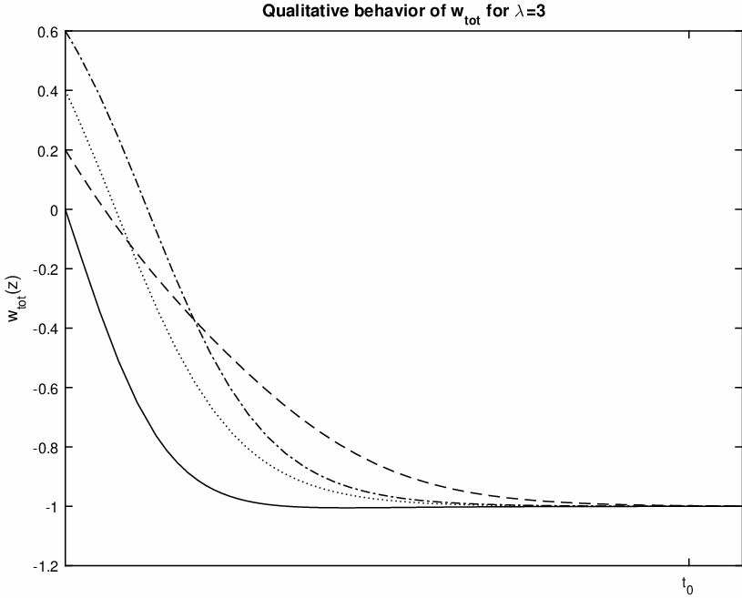
Finally the equation of state parameter for the total fluid, $w_{tot}=-1-\frac{2}{3}\frac{\dot{H}}{H^{2}}$ , is expressed as a function of $x,y,\lambda$ as follows

w_{tot}=1-\frac{2}{3}\lambda y.

(25)

We study the general evolution of the system (21)-(23) for the two cases: (a) $\lambda=const$ , which means $\bar{\Gamma}\left(\lambda\right)=0$ , i.e. $V\left(\phi\right)=V_{0}e^{-\lambda\phi}$ and (b) $\lambda\neq 0$ . In case (a) the system (21)-(23) reduces to a two-dimensional system.

III.1 Exponential potential

Consider now that $V\left(\phi\right)=V_{0}e^{-\lambda\phi}$ , which corresponds to the function

F\left(B\right)=-\frac{B}{\lambda}\left(\ln\left(-\frac{B}{\lambda}\right)-1\right).

(26)

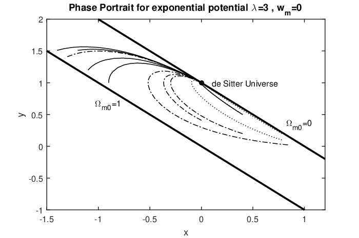
For that potential, the fixed points of the dynamical system, (21)-(22), are the points: $P_{A}~$ where $\left(x_{A},y_{A}\right)=\left(1,0\right)$ , $P_{B}$ with $\left(x_{B},y_{B}\right)=\left(\frac{3}{\lambda}\left(1+w\right),\frac{3}{2\lambda}\left(1-w\right)\right)$ and $P_{C}$ with coordinates $\left(x_{C},y_{C}\right)=\left(-\frac{6}{\lambda}+2,\frac{6}{\lambda}-1\right)$ . Specifically for each point we have:

•

Point $P_{A}$ corresponds to a universe without matter source; $\Omega_{m}=0$ and the total equation of state parameter is $w_{tot}=1$ , that is, the scalar field behaves like a stiff matter. The eigenvalues of the linearized system are calculated to be

$e_{1}^{A}=3\left(1-w_{m}\right),~e_{2}^{A}=6-\lambda.$ (27)

For the range $w_{m}\in[-1,1)$ , the eigenvalue $e_{1}^{A}$ is always positive. Hence the point is unstable.

•

At point $P_{B}$ the physical quantities are calculated to be $\Omega_{m}=1-\frac{3\left(3+w_{m}\right)}{2\lambda}$ and $w_{tot}=w_{m}$ . The point is well defined for $\lambda\geq\frac{\left(9+3w\right)}{2}$ . In that point the field $\phi$ mimics the matter source as the analogy of the exponential model in the minimally coupled cosmological scenario, which describes an accelerated universe for $w_{m}<-\frac{1}{3}$ .
The two eigenvalues of the linearized system are

	$\displaystyle e_{1}^{B}$	$\displaystyle=\frac{1}{4}\left(-3\left(1-w_{m}\right)-\sqrt{3}\sqrt{\left(1-w_{m}\right)\left(75+21w_{m}-16\lambda\right)}\right),$		(28)
	$\displaystyle e_{2}^{B}$	$\displaystyle=\frac{1}{4}\left(-3\left(1-w_{m}\right)+\sqrt{3}\sqrt{\left(1-w_{m}\right)\left(75+21w_{m}-16\lambda\right)}\right).$		(29)

For values of $w_{m}$ in the range $w_{m}\in[-1,1)$ , $\mathit{Re}\left(e_{1}^{B}\right)<0$ always holds. Furthermore for $\lambda\geq\frac{3}{16}\left(25+7w_{m}\right),~\lambda_{2}^{B}=\frac{3}{16}\left(25+7w_{m}\right)$ , $\mathit{Re}\left(e_{2}^{B}\right)=\mathit{Re}\left(e_{1}^{B}\right)<0$ holds, which means that the point is stable. However, if $\lambda<\lambda_{2}^{B}$ , the point is stable when $\lambda_{1}^{B}<\lambda<\lambda_{2}^{B}$ in which $\lambda_{1}^{B}=\frac{3}{2}\left(3+w_{m}\right)$ . Hence we conclude for $\lambda>\lambda_{1}^{B}$ the point $P_{B}$ is always stable.

•

Point $P_{C}$ describes a universe dominated by the field $\phi$ , where $\Omega_{m}=0$ and equation of state for the total fluid is $w_{tot}=\frac{1}{3}\left(2\lambda-9\right)$ , which describes an accelerated universe for $\lambda<\frac{9}{2}$ and describes a de Sitter universe for $\lambda=3~$ . The eigenvalues of the linearized system are

$e_{1}^{C}=-6+\lambda~,~e_{2}^{C}=-9-3w_{m}+2\lambda$ (30)

which gives that point is stable when $\lambda<6$ and $\lambda<\frac{3}{2}\left(3+w_{m}\right)$ . Furthermore if we consider that $w_{m}\in[0,1)$ then that point which describes an accelerated universe is always stable.

Table 1: Fixed points, cosmological parameters and stability for the dynamical system (23)-(23) with exponential potential

Point	$\left(\mathbf{x,y}\right)$	Existence	$\mathbf{\Omega}_{m}$	$\mathbf{w}_{tot}$	Acceleration	Stability
$\mathit{P}_{A}$	$\left(1,0\right)$	$\lambda\in\mathbb{R}$	$0$	$1$	No	Unstable
$\mathit{P}_{B}$	$\left(\frac{3}{\lambda}\left(1+w_{m}\right),\frac{3}{2\lambda}\left(1-w_{m}\right)\right)$	$\lambda\geq\frac{\left(9+3w\right)}{2}$	$1-\frac{3\left(3+w_{m}\right)}{2\lambda}$	$w_{m}$	$~w_{m}<-\frac{1}{3}$	$\lambda>\lambda_{1}^{B},~$
$\mathit{P}_{C}$	$\left(-\frac{6}{\lambda}+2,\frac{6}{\lambda}-1\right)$	$\lambda\in\mathbb{R}^{\ast}$	$0$	$\frac{1}{3}\left(2\lambda-9\right)$	$\lambda<\frac{9}{2}$	$\lambda<\frac{3}{2}\left(3+w\right)$

The fixed points and the values of the physical variables on these points are given in Table 1.

Refer to caption — Figure 1: Phase portrait for the potential $V\left(\phi\right)=\exp\left(-\lambda\phi\right)$ with $\lambda=-3$ and $w_{m}=0$ . The stable point is a de Sitter point. The left and right thick lines $y=1-x$ , and $y=-x$ , are the borders in which $0\leq\Omega_{m}\leq 1.$ The different lines describe different initial conditions $\left(x_{0},y_{0}\right)$ .

III.2 General potential

Consider now a general potential $V\left(\phi\right)$ , which corresponds to a general function $F\left(B\right)$ and in a general function $\bar{\Gamma}\left(\lambda\right)$ . Now, if there exists a value $\lambda=\lambda_{\ast}$ such as $\bar{\Gamma}\left(\lambda\right)=0$ , then from (21)-(22) we find the fixed points $\bar{P}_{A},~\bar{P}_{B}$ and $\bar{P}_{C}$ . The cosmological variables are the same as those of Table 1. However, the stability analysis is different. There are two more possibilities for which the system (21)-(23) admit stationary points, $x=0$ , or $\lambda=0$ , with $\lambda^{2}\bar{\Gamma}\left(\lambda\right)$ well defined.

For $x=0$ , we find that the rhs of (21)-(22) vanishes at the point $P_{D}$ with coordinates $\left(x,y,\lambda\right)=\left(0,1,3\right)$ while for $\lambda=0$ the fixed points are $P_{E}~,~\left(x,y,\lambda\right)=\left(1,0,0\right)$ , where the latter is a special case of the point $\bar{P}_{A}$ for $\lambda=0$ . As far as concerns the physical quantities at the point $P_{D}$ we have that $\Omega_{m}=0$ and $w_{tot}=-1$ , which means that $P_{D}$ is a de Sitter point. The stability of the points it follows

•

The eigenvalues of the linearized system around the point $\bar{P}_{A}$ are

\bar{e}_{1}^{A}=3\left(1-w_{m}\right)~,~\bar{e}_{2}^{A}=6-\lambda_{0}~,~\bar{e}_{3}^{A}=-\lambda_{0}^{2}\bar{\Gamma}_{,\lambda}\left(\lambda_{0}\right)

(31)

from which we can see that $\bar{e}_{1}^{A}$ is always positive for $w_{m}\in[-1,1)$ . Hence the point is always unstable.

•

For the point $\bar{P}_{B}$ the eigenvalues of the linearized system are

\bar{e}_{1}^{B}=\frac{1}{4}\left[-3\left(1-w_{m}\right)-\sqrt{3\Delta_{B}}\right]~~,~e_{2}^{\bar{B}}=\frac{1}{4}\left[-3\left(1-w_{m}\right)+\sqrt{3\Delta_{B}}\right]~

(32)

and

\bar{e}_{3}^{B}=-3\left(1+w_{m}\right)\lambda_{0}\bar{\Gamma}_{,\lambda}\left(\lambda_{0}\right),

(33)

where

\Delta_{B}=\left(1-w\right)\left(75+21w_{m}-16\lambda_{0}\right).

(34)

Eigenvalue $e_{3}^{B}$ is negative only when $\lambda_{0}\bar{\Gamma}_{,\lambda}\left(\lambda_{0}\right)>0$ . Now, for $\Delta_{B}\leq 0$ we have that $\mathit{Re}\left(\bar{e}_{1}^{B}\right)=\mathit{Re}\left(\bar{e}_{2}^{B}\right)<0$ , which means that the point is always stable. On the other hand for $\Delta_{B}>0$ , $\bar{e}_{1}^{B}<0$ holds and the point is stable when $e_{1}^{B}e_{2}^{B}>0$ , that gives

\frac{3}{2}\left(1-w_{m}\right)\left(9+3w_{m}-2\lambda_{0}\right)<0,

(35)

from which we find that $\bar{P}_{B}$ is stable when $\lambda_{0}>\frac{3}{2}\left(3+w_{m}\right)$ .

•

For the point $\bar{P}_{C}$ we find the eigenvalues

\bar{e}_{1}^{C}=-6+\lambda_{0}~,~\bar{e}_{2}^{C}=-9-3w_{m}+2\lambda_{0}~,~\bar{e}_{3}^{C}=-2\left(-3+\lambda_{0}\right)\bar{\Gamma}_{,\lambda}\left(\lambda_{0}\right)

(36)

from which the point is stable when $\lambda_{0}<\frac{3}{2}\left(3+w_{m}\right)$ and $\left(-3+\lambda_{0}\right)\bar{\Gamma}_{,\lambda}\left(\lambda_{0}\right)>0$ .

•

At the point $P_{D}$ the matrix of the linearized system has the following eigenvalues

e_{1}^{D}=\frac{3}{2}\left(-1-\sqrt{1-8\bar{\Gamma}\left(3\right)}\right),~e_{2}^{D}=\frac{3}{2}\left(-1+\sqrt{1-8\bar{\Gamma}\left(3\right)}\right)~,~e_{3}^{C}=-3\left(1+w_{m}\right)

(37)

which is a stable de Sitter point when $\mathit{Re}\left(\bar{\Gamma}\left[3\right]\right)>0$ . Note that $P_{D}$ is a special point of $P_{C}$ when $\lambda_{0}=3$ . However, the eigenvalues of the linearized system are different. That means that in a model with running $\lambda$ , the two points $P_{C}$ and $P_{D}$ can exist.

•

Finally the last point $P_{E}$ provides always a positive eigenvalue, that is, the point is always unstable.

We conclude that for a general potential a second stable de Sitter point exists which is stable for potentials in which $\bar{\Gamma}\left(3\right)>0$ . In general two de Sitter phases are possible, the points $P_{C}$ and $P_{D}$ . The above results are collected in Tables 2 and 3.

Table 2: Fixed points and cosmological parameters for the dynamical system (23)-(23) with arbitrary potential

Point	$\left(\mathbf{x,y,\lambda}\right)$	Existence	$\mathbf{\Omega}_{m}$	$\mathbf{w}_{tot}$	Acceleration
$\mathit{\bar{P}}_{A}$	$\left(1,0,\lambda_{0}\right)$	$\lambda_{0}\in\mathbb{R}~,~\bar{\Gamma}\left(\lambda_{0}\right)=0$	$0$	$+1$	No
$\mathit{\bar{P}}_{B}$	$\left(\frac{3}{\lambda}\left(1+w_{m}\right),\frac{3}{2\lambda}\left(1-w_{m}\right),\lambda_{0}\right)$	$\lambda_{0}\geq\frac{\left(9+3w\right)}{2}~,\bar{\Gamma}\left(\lambda_{0}\right)=0$	$1-\frac{3\left(3+w_{m}\right)}{2\lambda}$	$w_{m}$	$~w_{m}<-\frac{1}{3}$
$\mathit{P}_{C}$	$\left(-\frac{6}{\lambda}+2,\frac{6}{\lambda}-1,\lambda_{0}\right)$	$\lambda_{0}\in\mathbb{R}^{\ast}~,~\bar{\Gamma}\left(\lambda_{0}\right)=0$	$0$	$\frac{1}{3}\left(2\lambda-9\right)$	$\lambda_{\ast}<\frac{9}{2}$
$\mathit{P}_{D}$	$\left(0,1,3\right)$	Always	$0$	$-1$	Yes
$\mathit{P}_{E}$	$\left(1,0,0\right)$	Always	$0$	$+1$	No

Table 3: Eigenvalues and stability for the critical points of the dynamical system (23)-(23) with arbitrary potential

Point/Eigenv.	$\mathbf{e}_{1}$	$\mathbf{e}_{2}$	$\mathbf{e}_{3}$	Stability
$\mathit{\bar{P}}_{A}$	$3\left(1-w_{m}\right)$	$6-\lambda_{0}$	$-\lambda_{0}^{2}\bar{\Gamma}_{,\lambda}\left(\lambda_{0}\right)$	Unstable
$\mathit{\bar{P}}_{B}$	$\frac{1}{4}\left[-3\left(1-w_{m}\right)-\sqrt{3\Delta_{B}}\right]$	$\frac{1}{4}\left[-3\left(1-w_{m}\right)+\sqrt{3\Delta_{B}}\right]$	$-3\left(1+w_{m}\right)\lambda_{0}\bar{\Gamma}_{,\lambda}\left(\lambda_{0}\right)$	$\lambda_{0}>\frac{3}{2}\left(3+w_{m}\right)$
$\mathit{P}_{C}$	$-6+\lambda_{0}$	$-9-3w_{m}+2\lambda_{0}$	$-2\left(-3+\lambda_{0}\right)\bar{\Gamma}_{,\lambda}\left(\lambda_{0}\right)$	$\begin{array}[c]{c}\lambda_{0}<\frac{3}{2}\left(3+w_{m}\right),\\ \left(-3+\lambda_{0}\right)\bar{\Gamma}_{,\lambda}\left(\lambda_{0}\right)>0\end{array}$
$\mathit{P}_{D}$	$\frac{3}{2}\left(-1-\sqrt{1-8\bar{\Gamma}\left(3\right)}\right)$	$\frac{3}{2}\left(-1+\sqrt{1-8\bar{\Gamma}\left(3\right)}\right)$	$-3\left(1+w_{m}\right)$	$\mathit{Re}\left(\bar{\Gamma}\left[3\right]\right)>0$
$\mathit{P}_{E}$	$3\left(1-w_{m}\right)$	$6$	$0$	Unstable

As a special example consider the potential $V\left(\phi\right)=V_{0}e^{-\sigma\phi}+V_{1}$ , from which we have

F\left(B\right)=-\frac{B}{\lambda}\left(\ln\left(-\frac{B}{\lambda}\right)-1\right)+V_{1}\text{.}

(38)

For that potential we have that $\phi=-\frac{1}{\sigma}\ln\left(\frac{\lambda\bar{V}_{0}}{\sigma-\lambda}\right),~\bar{V}_{0}=\frac{V_{1}}{V_{0}}$ and $\bar{\Gamma}\left(\lambda\right)=-1-\frac{1}{\bar{V}_{0}}\left(1-\frac{\sigma}{\lambda}\right)$ . For the point $P_{C}$ we find that $\lambda_{0}=\frac{\sigma}{1+\bar{V}_{0}}$ . Hence $P_{C}$ is stable when

\lambda_{0}<\frac{3}{2}\left(3+w_{m}\right)~~\text{and~}-\left(-3+\lambda_{0}\right)\frac{\sigma}{\lambda_{0}^{2}\bar{V}_{0}}>0.

(39)

Hence, if $3<\lambda_{0}<$ $\frac{3}{2}\left(3+w_{m}\right)$ , then $\frac{\sigma}{\bar{V}_{0}}<0$ while for $\lambda_{0}<3~$ the point is stable when $\frac{\sigma}{V_{0}}>0$ . On the other hand point $P_{D}$ is stable when

	$\displaystyle\sigma$	$\displaystyle<-3\left(1+\bar{V}_{0}\right)~\ \text{for }\bar{V}_{0}>0,$		(40)
	$\displaystyle\sigma$	$\displaystyle>-3\left(1+\bar{V}_{0}\right)~\text{~for }\bar{V}_{0}<0.$		(41)

In the following section we proceed with the derivation of some analytical solutions for the field equations (14)-(17).

IV Exact cosmological solutions

We consider that in the field equations (14)-(17) the matter source corresponds to that of a dust fluid, i.e. $w_{m}=0$ , and $p_{m}=0$ . Hence (17) provides $\rho_{m}=\rho_{m0}a^{-3}$ . Furthermore for the potential, $V\left(\phi\right)$ , we consider that $V_{1}\left(\phi\right)=V_{0}\exp\left(-3\phi\right)$ , which leads to a de Sitter universe and $V_{2}\left(\phi\right)=V_{0}\exp\left(-3\phi\right)-2\Lambda,~$ . According to the above this has two de Sitter phases, points $P_{C}$ and $P_{D}$ .

IV.1 Solution for $V\left(\phi\right)=V_{0}\exp\left(-3\phi\right)$

For the potential $V_{1}\left(\phi\right)$ the Lagrangian of the field equations becomes

\mathcal{L}\left(a,\dot{a},\phi,\dot{\phi}\right)=-6a\dot{a}^{2}+6a^{2}\dot{a}\dot{\phi}\,-a^{3}V_{0}e^{-3\phi}

(42)

so that the field equations are the Euler-Lagrange equations of (42) with respect to the variables $\left\{a,\phi\right\},$ while the first modified Friedmann’s equations can be seen as the Hamiltonian function of (42), $~\mathcal{H}=E,$ where now $\rho_{m0}=2\left|E\right|.$

It is straightforward to see that (42) admits the two extra Noetherian conservation law⁴⁴ 4 For the application of point symmetries in cosmological studies see [56, 57, 58] and references therein while a partial classification of Noether point symmetries in $f\left(T,B\right)$ can be found in [59] which are

I_{1}=\dot{\phi}-\frac{\dot{a}}{a}~\mbox{\rm and}~I_{2}=t\left(\dot{\phi}-\frac{\dot{a}}{a}\right)-\left(\phi-\ln a\right).

(43)

We perform the coordinate transformation $a=u^{\frac{1}{3}},~\phi=v-\frac{1}{3}\ln\left(u\right)$ . In the new coordinates Lagrangian (42) is written

L\left(u,\dot{u},v,\dot{v}\right)=2\dot{u}\dot{v}-V_{0}e^{-3v}

(44)

and the field equations are taking the simple form

2\dot{u}\dot{v}+V_{0}e^{-3v}=2E,

(45)

\ddot{u}-\frac{3}{2}V_{0}e^{-3v}=0~\mbox{\rm and}~\ddot{v}=0.

(46)

Finally the solution is given in a closed-form expression as follows

u\left(t\right)=\frac{\bar{V}_{0}}{9v_{1}^{2}}e^{-3v_{1}t}+u_{1}t+u_{0},

(47)

where $\bar{V}_{0}=\frac{3}{2}V_{0}e^{-3v_{0}}$ and $E=u_{1}v_{1}$ . We have that the de Sitter phase is recovered when $v_{1}<0$ . From (47) it follows that the scale factor has the form

a^{3}\left(t\right)=a_{2}e^{\beta t}+a_{1}t+a_{0},

(48)

where the spacetime has a singularity at $t=0$ when $a_{0}=-a_{2}$ , that is, the scale factor becomes $a^{3}\left(t\right)=a_{2}\left(e^{\beta t}-1\right)+a_{1}t$ .

Moreover, in the vacuum solution in which $u_{1}v_{1}=0$ , we have two possibilities: $u_{1}=0$ or $v_{1}=0$ . For the latter case, that is $\beta=0$ , the solution is $a\left(t\right)\simeq t^{\frac{1}{3}}$ , which corresponds to the solution of GR with a perfect fluid with equation of state parameter $w=-\frac{1}{3}$ .

However, in the latter case for which $u_{1}=0$ i.e., $a_{1}=0$ , the scale factor with $a\left(t\rightarrow 0\right)=0$ is of the form

a^{3}\left(t\right)=a_{2}\left(e^{\beta t}-1\right).

(49)

Easily we have that $t=\frac{1}{\beta}\ln\left(1+\frac{a^{3}}{a_{2}}\right)$ , from which we calculate the Hubble Function

\left(H\left(a\right)\right)^{2}=\frac{\beta^{2}}{9}+\frac{2\beta^{2}}{9}a_{2}a^{-3}+\frac{\beta^{2}}{9}\left(a_{2}\right)^{2}a^{-6}.

(50)

This means that the theory provides us with a cosmological constant term, a dust term and a stiff fluid, equivalently with that of the minimally coupled scalar field [60].

IV.2 Solution for $V\left(\phi\right)=V_{0}\exp\left(-3\phi\right)-2\Lambda$

As a second potential we consider the same as the above where now we include a cosmological constant term. It is easy to see that in the coordinate system $\left\{u,v\right\}$ the field equations become

2\dot{u}\dot{v}+V_{0}e^{-3v}-2\Lambda u=2E

(51)

and

\ddot{u}-\frac{3}{2}V_{0}e^{-3v}=0~,~\ddot{v}-\Lambda=0,

(52)

from which we have that the scale factor is expressed in terms of the error function, $\mathcal{E}\left(t\right)$ , as

	$\displaystyle a^{3}\left(t\right)$	$\displaystyle=\frac{\bar{V}_{1}}{3\Lambda}\exp\left(-\frac{3}{2}\Lambda t^{2}-3v_{1}t\right)+$		(53)
		$\displaystyle+\frac{\sqrt{6\pi}\bar{V}_{1}}{6\Lambda^{\frac{3}{2}}}\left(\Lambda t+v_{1}\right)\mathcal{E}\left(\frac{\sqrt{6}}{2\Lambda}\left(\Lambda t+v_{1}\right)\right)+u_{1}t+u_{2},$		(54)

where $\bar{V}_{1}=V_{0}e^{-3v_{0}}$ and $v\left(t\right)=\frac{\Lambda}{2}t^{2}+v_{1}t+v_{0}$ .

The reason that this is possible is that the Lagrangian of the field equations admits a Noetherian conservation law which is not generated by point symmetries as in the potential $V_{1}\left(\phi\right)$ but from generalized symmetries. In particular the Killing tensor of the minisuperspace provides a contact symmetry (see [61] and references therein).

V Conclusions

In the context of modified theory of gravities we considered a gravitational theory in which the deviation from General Relativity is given by a function of the boundary term which relates the Ricci Scalar, $R$ , and the invariant, $T$ , of teleparallel gravity. The theory that we considered is a fourth-order theory and in the case of an isotropic and homogeneous universe the field equations can be written as a (constraint) Hamiltonian system with two degrees of freedom. One degree of freedom corresponds to the scalar factor of the geometry and the second one is a field which describes the higher-order derivatives, as in the case of $f\left(R\right)$ -gravity. The theory admits a constraint and it is the equation of motion which corresponds to the lapse function of the geometry.

Though that theory is a fourth-order theory differs from $f\left(R\right)$ -gravity and the field which is introduced from the application of the Lagrange multipliers does not describe a scalar tensor theory. The minisuperspace Lagrangian is given by

\mathcal{L}\left(a,\dot{a},\phi,\dot{\phi}\right)=-\frac{6}{N}a\dot{a}^{2}+\frac{6}{N}a^{2}\dot{a}\dot{\phi}+Na^{3}V\left(\phi\right).

(55)

However, under the change $a=Ae^{\frac{\phi}{2}}$ and $N=e^{\frac{3\phi}{2}}n$ , this Lagrangian becomes

\mathcal{L}\left(A,\dot{A},\phi,\dot{\phi}\right)=-\frac{6}{n}A\dot{A}^{2}+\frac{3}{2n}A^{3}\dot{\phi}^{2}+na^{3}\left(e^{3\phi}V\left(\phi\right)\right)

(56)

which is the Lagrangian of a canonical minimally coupled (phantom) scalar field with potential $U\left(\phi\right)=e^{3\phi}V\left(\phi\right)$ . It is easy to see that the transformation $\left(N,a\right)\rightarrow\left(e^{\frac{3\phi}{2}}n,Ae^{\frac{\phi}{2}}\right)$ does not relate conformal equivalent theories, such as in the scalar-tensor theories. However, the relation between the two Lagrangians, (55) and (56), is important because the analysis of [62] can be applied and it can be easily shown that the gravitational field equations (14)-(16) form an integrable dynamical system.

In order to study the effects which follow from the new terms in the dynamics of the field equations the critical points were calculated. Every point corresponds to a physical state and the physical parameters were calculated. The importance of the existence of the points is that for families of initial conditions the evolution of the universe passes closely to the physical states which are described from the points (unstable points) or at the end reach the solution which is described by the critical point (stable point). In our analysis we found that for it is possible to have a theory which provides a matter era (unstable point) and two acceleration phases in which the one can be stable and the other unstable. This is an interesting result and it is different from that of $f\left(R\right)$ -gravity. Moreover some closed-form solutions were derived and the explicitly form of the FLRW spacetime was found.

There are various open questions which have to be answered for that consideration, but the property that the only constraint in the field equations is that of the “Hamiltonian” is essential because various methods can be applied, from the scalar field description, in order to study the theory. In a future work we would like to extend the present analysis in order to search for other kinds of cosmological solutions and extend the analysis of the critical points at the infinite region. The existence of static-spherical solution is also of special interests.

Acknowledgements.

I acknowledge the financial support of FONDECYT grant no. 3160121 and I thank the Durban University of Technology and the University of KwaZulu-Natal for the hospitality provided while part of this work was performed.

References

[1] M. Tegmark et al., Astrophys. J. 606, 702 (2004)
[2] M. Kowalski et al., Astrophys. J. 686, 749 (2008)
[3] E. Komatsu et al., Astrophys. J. Suppl. Ser. 180, 330 (2009)
[4] P. A. R. Ade et al., (Planck Collaboration), Astron. Astroph. 594, A13 (2016)
[5] B. Ratra and P.J.E Peebles, Phys. Rev. D 37, 3406 (1988)
[6] J.D. Barrow and P. Saich, Class. Quant. Grav. 10, 279 (1993)
[7] E.V Linder, Phys. Rev. D. 70, 023511 (2004)
[8] J.M. Overduin and F.I. Cooperstock, Phys. Rev. D 58, 043506 (1998)
[9] M.C. Bento, O. Bertolami and A.A. Sen, Phys. Rev. D 66, 043507 (2002)
[10] A. Yu. Kamenshchik, U. Moschella and V. Pasquier, Phys. Lett. B 511, 265 (2001)
[11] N. Chow and J. Khoury, Phys. Rev. D 80, 024037 (2009)
[12] A. De Felice and S. Tsujikawa, Phys. Rev. D 84, 124029 (2011)
[13] A. Paliathanasis, S. Pan, S. Pramanik, Class. Quant. Grav. 32, 245006 (2015)
[14] C. Brans and R.H. Dicke, Phys. Rev. 124, 195 (1961)
[15] H.A. Buchdahl, Mon. Not. Roy. Astron. Soc. 150, 1 (1970)
[16] T.P. Sotiriou and V. Faraoni Rev. Mod. Phys. 82, 451 (2010)
[17] S. Nojiri and S.D. Odintsov, Phys. Rep. 505, 59 (2011)
[18] S. Capozziello and M. Franvaviglia, Gen. Relativ. Gravit. 40, 357 (2008)
[19] R. Ferraro and F. Fiorini, Phys. Rev. D 75, 084031 (2007)
[20] R. Ferraro and F. Fiorini, Phys. Rev. D 78, 124019 (2008)
[21] S. Basilakos, A.P. Kouretsis, E.N. Saridakis and P.C. Stavrinos, Phys. Rev. D 88, 123510 (2013)
[22] G. Kofinas and M. Tsoukalas, Eur. Phys. J. C 76, 686 (2016)
[23] R. Myrzakulov and L. Sebastiani, Astro. Sp. Sci. 361, 188 (2016)
[24] S. Nojiri and S.D. Odintsov, Phys. Rev. D 74, 086005 (2006)
[25] S. Nojiri and S.D. Odintsov, Phys. Rev. D 68, 123512 (2003)
[26] K.-i. Maeda and N. Ohta, Phys. Lett. B 597, 400 (2004)
[27] K. Bamba, Z.-K. Guo and N. Ohta, Prog. Theor. Phys. 118, 879 (2007)
[28] S. Capozziello, Int. J. Mod. Phys. D 11, 483 (2002)
[29] P. A. R. Ade et al., (Planck Collaboration), Astron. Astroph. 594, A14 (2016)
[30] Z. Gironés, A. Marchetti, O. Mena, C. Péna-Garay and N. Rius, JCAP, 2010 11 (2010)
[31] J. Bel, P. Brax, C. Marinoni and P. Valageas, Phys. Rev. D 91 103503 (2015)
[32] R.C. Nunes, A. Bonilla, S. Pan and E.N. Saridakis, JCAP 08, 011 (2016)
[33] K. Koyama, Rept. Prog. Phys. 79, 046902 (2016)
[34] T. Chiba, T.L. Smith and A.L. Erickcek, Phys. Rev. D 75, 124014 (2007)
[35] C.P.L. Berry and J.R. Gair, Phys. Rev. D 83, 104022 (2011)
[36] P. Wu, H.W. Yu, Phys. Lett. B 693, 415 (2010)
[37] L. Iorio, N. Radicella and M.L. Ruggiero, JCAP 2015, 08 (2015)
[38] K. Hayashi and T. Shirafuji, Phys. Rev. D 19, 3524 (1979)
[39] A. Einstein 1928, Sitz. Preuss. Akad. Wiss. p. 217; ibid p. 224 [Translated by A. Unzicker and T. Case, (preprint: arXiv: physics/0503046)]
[40] B. Li, T.P. Sotiriou and J.D. Barrow, Phys. Rev. D 83, 064035 (2011)
[41] N. Tamanini and C.G. Bohmer, Phys. Rev D 86, 044009 (2012)
[42] B. Li, J.D. Barrow and D.F. Mota, Phys. Rev. D 76, 044027 (2007)
[43] S. Nojiri and S.D. Odintsov, Phys. Lett. B 631, 1 (2005)
[44] G. Cognola, E. Elizalde, S. Nojiri, S.D. Odintsov and S. Zerbini, Phys. Rev. D 73, 084007 (2006)
[45] A. De Felice, J.-M. Gerard and T. Suyama, Phys. Rev. D 82, 063526 (2010)
[46] T. Harko, F.S.N. Lobo, S. Nojiri and S.D. Odintsov, Phys. Rev. D 84, 024020 (2011)
[47] R. Myrzakulov, EPJC 72, 1 (2012)
[48] S. Bahamonde, C. G. Bohmer and M. Wright, Phys. Rev. D 92, 104042 (2015)
[49] M. Krššák and E.N. Saridakis, Class. Quant. Grav. 33, 115009 (2016)
[50] J. O’Hanlon, Phys. Rev. Lett. 29 137 (1972)
[51] D. Wands, Class. Quantum Grav. 11, 269 (1994)
[52] E.J. Copeland, A.R. Liddle and D. Wands, Phys. Rev. D. 57, 4686 (1998)
[53] R. Lazkoz, G. Leon and I. Quiros, Phys. Lett. B 649, 103 (2007)
[54] C.R. Fadragas and G. Leon, Class. Quant. Gravit. 31, 195011 (2014)
[55] L. Amendola, D. Polarski and S. Tsujikawa, Phys. Rev. Lett. 98, 131302 (2007)
[56] S. Capozziello, R. de Ritis, C. Rubano, Phys.Lett. A 177, 8 (1993)
[57] S. Basilakos, S. Capozziello, M. De Laurentis, A. Paliathanasis and M. Tsamparlis, Phys. Rev. D 88, 103526 (2013)
[58] P.A. Terzis, N. Dimakis and T. Christodoulakis, Phys. Rev. D. 90, 123543 (2014)
[59] S. Bahamonte and S. Capozziello, EPJC 77, 107 (2017)
[60] A. Paliathanasis, M. Tsamparlis, S. Basilakos and J.D. Barrow, Phys. Rev. D 91, 123535 (2015)
[61] A. Paliathanasis, Class. Quantum Gravit. 33, 075012 (2016)
[62] N. Dimakis, A. Karagiorgos, A. Zampeli, A. Paliathanasis, T. Christodoulakis and P.A. Terzis, Phys. Rev. D 93, 123518 (2016)