Topological Distances between Networks
and Its Application to Brain Imaging
Abstract
This paper surveys various distance measures for networks and graphs that were introduced in persistent homology. The scope of the paper is limited to network distances that were actually used in brain networks but the methods can be easily adapted to any weighted graph in other fields. The network version of Gromov-Hausdorff, bottleneck, kernel distances are introduced. We also introduce a recently developed KS-test like distance based on monotonic topology features such as the zeroth Betti number. Numerous toy examples and the result of applying many different distances to the brain networks of different clinical status and populations are given.
1 Introduction
There are many statistically oriented similarity measures and distances between networks in literature [5, 16, 47]. Many of these approaches simply ignore the topology of the networks and mainly use the sum of differences between either node or link measurements or correlations. These network distances are sensitive to the topology of networks. They may lose sensitivity over topological structures such as the connected components or holes in the network.
In graph theoretic approaches, the similarity and distance of networks are measured by determining the difference in graph theory features such as assortativity, betweenness centrality, small-worldness and network homogeneity [12, 51, 57]. Comparison of graph theory features appears to reveal changes of structural or functional connectivity associated with different clinical populations [51]. Since weighted brain networks are difficult to interpret and visualize, they are often turned into binary networks by thresholding edge weights [32, 60]. However, the choice of thresholding the edge weights may alter the network topology. To obtain the proper optimal threshold, the multiple comparison correction over every possible edge has been proposed [9, 17, 29, 50, 52, 60]. However, depending on what -value to threshold, the resulting binary graph also changes. Others tried to control the sparsity of edges in the network in obtaining the binary network [1, 7, 32, 37, 45, 58, 60]. But then one encounters the problem of thresholding sparse parameters. Thus existing methods for binarizing weighted networks have been circular. Until now, there are not widely accepted criteria for thresholding networks. Instead of trying to come up with a proper threshold for network construction that may not work for different clinical populations or cognitive conditions [60], why not use all networks for every possible threshold? Motivated by this question, new multiscale hierarchical network modeling framework based on persistent homology has been developed recently [20, 21, 38, 39, 41].
Persistent homology, a branch of computational topology [13, 25], provides a more coherent mathematical framework to measuring network distance than the conventional method of simply taking difference between graph theoretic features. Instead of looking at networks at a fixed scale, as usually done in many standard brain network analysis, persistent homology observes the changes of topological features of the network over multiple resolutions and scales [26, 34, 62]. In doing so, it reveals the most persistent topological features that are robust under noise perturbations. This robustness in performance under different scales is needed for most network distancs that are parameter and scale dependent.
In persistent homological network analysis as established in [38, 41], instead of analyzing networks at one fixed threshold that may not be optimal, we build the collection of nested networks over every possible threshold using a graph filtration, a persistent homological construct [20, 41]. The graph filtration is a threshold-free framework for analyzing a family of graphs but requires hierarchically building specific nested subgraph structures. The proposed method share some similarities to the existing multi-thresholding or multi-resolution network models that use many different arbitrary thresholds or scales [2, 32, 35, 41, 55]. Such approaches are mainly used to visually display the dynamic pattern of how graph theoretic features change over different thresholds and the pattern of change is rarely quantified. Persistent homology can be used to quantify such dynamic pattern in a more coherent quantifiable way.
In persistent homology, there are various metrics that have been proposed to measure distance between topological spaces. The bottleneck distance is perhaps the most widely used distance measure in persistent homology [24, 23]. The bottleneck distance was originally defined for measuring the distance between two sets in the same metric space. The method was later adapted to measure the difference between two persistence diagrams [26]. Despite the strong mathematical motivation from differential geometry, they are not intuitive, as points in different persistence diagrams (PD) do not naturally correspond as a bijection. Thus, the computation of the distances between PDs is not straightforward [23, 33, 44]. [19] bypassed the problem of comparing PDs by that of comparing the density of points in a squre grid via kernel smoothing. Motivated by [19], later theories and applications of inference on PDs have taken the direction of kernel distances [46, 49, 40]. The kernel itself is an inner product; thus, it naturally yields a Hilbert space structure. Subsequently, other Hilberst space tools such as principle component analysis or support vector machine can be easily applied. In [49], persistent scale space (PSS) kernel, which is the inner product of heat diffusions with the PD points as the initial heat sources, is introduced. PSS is later extended to multiple PSS kernels in determining the changes in brain network distances in aging [40].
Gromov-Hausdorff (GH) distance is also another popular distance that is originally used to measure distance between two metric spaces [56]. It was later adapted to measure distances in persistent homology and dendrograms [13, 14, 15]. Subsequently, it was applied to brain networks [38, 41]. In the case of brain networks, we often have prior node-to-node correspondences established by image registration. Thus, the computation of GH-distance is simplified to the differences in single linkage matrices. This connects GH-distance to popular hierarchical clustering.
All the above network distances do not have known probability distributions. The statistical inferences on distances have been done through resampling techniques such as jackknife, bootstraps or permutations [41, 42, 21], which often cause computational bottlenecks for large scale networks. To bypass the computational bottleneck associated with resampling large scale networks, the Kolmogorove-Smirnov (KS) test like distance was first proposed in [18, 20]. Later it was also used in characterizing the multidimensional graph filtration in multimodal brain imaging study [42]. The advantage of using KS-test like distance is its easy to interpret compared to other less intuitive distances. Due to its simplicity, it is possible to enumerate the possible sample space combinatorially and determine its probability distribution exactly without estimating the distribution empirically by resampling techniques [22].
Many distance or similarity measures are not metrics but having metric distances makes the interpretation of brain networks easier due to the triangle inequality. Many network distances are in fact metric or ultrametric [41]. Let us start with the review of metric space and formulate networks as metric spaces.
2 Network as a metric space
Consider a weighted graph or network with the node set and the edge weights , where is the weight between nodes and . The edge weight is usually given by a similarity measure between the observed data on the nodes. Various similarity measures have been proposed. The correlation or mutual information between measurements for the biological or metabolic network and the frequency of contact between actors for the social network have been used as edge weights [6, 8].
We will assume that the edge weights satisfy the metric properties: nonnegativity, identity, symmetry and the triangle inequality such that
With theses conditions, forms a metric space. Many real-world networks satisfy the metric properties. Although the metric property is not necessary for building a network, it offers many nice mathematical properties and easier interpretation on network connectivity.
Example 1
Suppose we have measurement vector on the node (Fig. 1). The weights between nodes is often given by some bivariate function on and , i.e., . Denote the correlation between and as . If the weights are given by , forms a metric space.

Example 2
Suppose we center and rescale the measurement such that . Denote the full data matrix as . The edge weight of network is then often given by some function of , i.e., . For instance, the correlation between the nodes and is given by and is the correlation matrix. The correlation is invariant under centering and scaling. Such operations are often done in practice to speed up the computation in sparse learning [43, 20, 21].
Under centering and scaling, does not satisfy the the triangle inequality. This is easily seen from the counter example
| (1) |
which satisfies
and results in . is not a metric, but is a metric.
Even though, the centered and rescaled correlation is no longer a metric in the Euclidean space, it may be a metric in some high dimensional non-Euclidean space.
Example 3
Under centering and scaling, we can allegorically show that is a metric. This is equivalent to saying that is a metric on the -dimensional unit sphere. It obtains minimum when and maximum when .
3 Matrix norm as a network distance
Matrix norm of the difference between networks is often used as measure of similarity between networks [5, 61]. Given two networks and , the -norm of network difference is given by
| (2) |
and are most often used and they are referred to as -distance and Euclidean distance (). -distance, often referred to as Frobenius norm distance, is probability the most often used matrix similarity measure [61] and can be rewritten as
If are adjacency matrices, -distance is the Hamming metric often used in information theory [5]. When -distance is written as
| (3) |
(3) is a special case of Gromov-Hausdorff (GH) distance and related to type-I error estimation under multiple comparisons [18, 42].
The idea of using spherical geodesics in constructing the metric space in Example 3 can be further extended to other abstract spaces. Consider a collection of positive definite symmetric matrices of size , which is denoted as . Many brain connectivity matrices including correlation and covariance metrics belong to [48]. Given edge weights , the shortest distance between and in this manifold is given by the log-Euclidean distance [4]
where is the matrix logarithm. The log-Euclidean distance can be viewed as the generalized manifold version of Frobenius norm distance.
The element-wise differences may not capture additional higher order similarity. For instance, there might be relations between a pair of columns or rows [61]. Further, -distances usually surfer the problem of outliers. Since all the edges are assigned equal weights, few outlying extreme edge weights may severely affect the distance more than needed. Further, because they compare each edges separately, these distances simply ignore the underlying topological structures. It is necessary to define distances that are more topological in nature.

Example 4
The insufficiency of network distances is illustrated in Fig. 2. Networks were simulated from the baseline network with two connected components. Networks were simulated from the baseline network with one connected component (Fig. 2-(a)). Each network has 100 nodes and their edge weights are given by the Euclidean distance between nodes (b). The pairwise distance between 100 networks based on -, -, -distances, and 1 - Pearson correlation are shown in (c). Ward hierarchical clustering [38, 59] into two groups gives the clustering accuracy of 53 %, 52 %, 55 %, and 50 %. The distances and correlations ignore the topological information of connectedness and result in extremely poor performance, which is no different from randomly flipping coins. This example demonstrates the need for topologically more aware distances in networks.
4 Network and graph filtrations
To define topological distance in weighted networks in persistent homology, it is necessary to construct a filtration. Let us threshold edge weights and binarize a weighted network.
Definition 1
Given weighted network , the binary network is a graph consisting of the node set and the edge weight given by
| (4) |

Note is the adjacency matrix of . The binary network is a simplicial complex consisting of -simplices (nodes) and -simplices (edges) [28, 30]. In the metric space , the Rips complex is a simplicial complex whose -simplices correspond to unordered -tuples of points that satisfy in a pairwise fashion [30]. While the binary network has at most 1-simplices, the Rips complex can have at most -simplices (Fig. 3). Thus, we have . The Rips complex has the property that
for When , the Rips complex is simply the node set . By increasing the filtration value , we are connecting more nodes so the size of the edge set increases. Such the nested sequence of the Rips complexes is called a Rips filtration, the main object of interest in the persistent homology [26].
Since a binary network is a special case of the Rips complex, it inherits all the topological properties of the Rips complex including filtration
for The sequence of such nested multiscale graph structure is called the graph filtration [38, 41].
Example 5
Fig. 4 shows an example of a graph filtration in fluorodeoxyglucose (FDG) positron emission tomography (PET) study of three different populations [41]. Graph filtrations of the inter-subject correlation in FDG-PET measurements showing group differences between attention-deficit hyperactivity disorder (ADHD), autism spectrum disorder (ASD) children and pediatric controls (PedCon). The Pearson correlation is used as filtration values. PedCon clearly shows much dense brain connectivity over the filtration.

If we order the edge weights in an increasing order, we have the sorted edge weights:
where , the maximum possible number of edge weights. The subscript denotes the order statistic.
Due to multiplicity of edge weights, the filtration
may not be unique in a sense we can easily have for some . To avoid this redundancy, we sort and remove any multiplicative weights and obtain the set of unique positive weights
The graph filtration on this unique edge set will be unique:
Theorem 4.1
For graph with distinct edge weights can be uniquely decomposed as the graph filtration
| (5) |
The proof of uniqueness is given in [21]. For any , belongs to one of the binary network in the filtration (5). In this sense, the representation (5) is unique. The edge weights can be recovered from the filtration and the filtration values. Let if nodes and are connected in binary network and otherwise. Then
The finiteness and uniqueness of the filtration over weighted graphs are intuitively clear by themselves and are already applied in software packages such as javaPlex [3].
5 Bottleneck distance
The network topology can be represented by the birth and death of homology groups in persistent homology. The zeroth and first homology groups are a set of connected components and holes, respectively. During a filtration, homologies in homology group appear and disappear. If a homology appears at the threshold and disappears at it can be encoded into a point, in . If number of homologies appear during the filtration of a network , the homology group can be represented by a point set
This scatter plot is called the persistence diagram (PD) [24]. Note that the Betti number is the cardinality of homology group at the fixed threshold, while is the number of homologies that appear during the filtration.
Given two networks and we construct the corresponding graph filtrations. Subsequently,PDs
and
are obtained through the filtration.
The bottleneck distance between networks is defined as the bottleneck distance of the corresponding PDs:
| (6) |
where , and is a bijection from to . If , the infinity norm is defined as Note (6) assumes such that the bijection exists. If , there is no one-to-one correspondence between two PDs. Then, auxiliary points
and
that are orthogonal projections to the diagonal line of points in and are added to to respectively to make the identical number of points in PDs. The bijection is determined by the bipartite graph matching algorithm [24]. Since is a one-to-one correspondence with the minimum sum of distances, points that are close to the diagonal line, i.e., those with small durations, are predominantly mapped to auxiliary points. Thus, the auxiliary points are usually ignored during the estimation of bottleneck distance. This is consistent with the premise of persistent homology that homology with a longer duration is a signal of the topological space, but homology with a shorter duration is noise.

Example 6
Examples of bottleneck distance are shown in Fig. 5. Given four topological spaces and the PDs of connected components and holes are shown in (b). The bottleneck distance can easily distinguish (one connected component) from (three connected components) as shown in (c)-left. When it is applied to the PDs of holes, it can easily distinguish (no hole) from (three holes) as shown in (c)-right.
Example 7
When the bottleneck distance is applied to 100 simulated networks in Example 4, the networks are clustered according to two baseline topological structures with 100 % accuracy. The superior almost perfect performance is due to the fact that the bottleneck distance use the topological information of connectedness represented in PD.
6 Kernel distance
A multi-scale kernel method for PDs based on state space theory has been proposed in [46, 49]. It embeds the topological information in PD into a feature space by kernel smoothing of PD :
where is the mirror reflection of with respect to the diagonal line. Then the inner product between two PDs is given by kernel
is called the persistence state-space (PSS) kernel. Kernel distance is then defined as a distance between PDs in a feature space [53]:
The performance of kernel distance depends on the parameter Thus, should be chosen carefully.
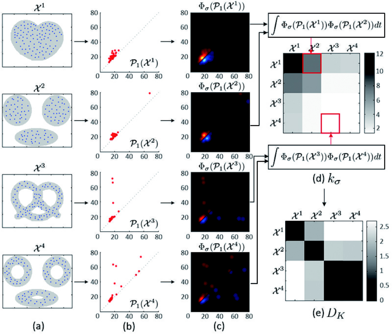
Example 8
The bottleneck distance does not take into account the difference in the number of connected components or holes since it compares two PDs through a one-to-one correspondence. However, the kernel distance estimates the difference of all pairs of points in two PDs. Moreover, the bottleneck distance tends to ignore points that are close to the diagonal line in PD by mapping to auxiliary points although such points may sometimes indicate the underlying topological structure that discriminates topological spaces.
7 Gromov-Hausdorff distance
The change of connected components during the filtration has an agglomerative hierarchical clustering structure based on single linkage [13, 14, 41]. Each node starts as a single connected component, and pairs of connected components then are merged if the distance between the closest nodes in two disjoint connected components is smaller than the filtration value. The distance between the closest nodes in the two disjoint connected components and is called the single linkage distance (SLD), which is defined as
Thus, every edge connecting a node in to a node in has the same SLD. SLD is then used to construct the single linkage matrix (SLM) (Fig. 7). SLM shows how connected components are merged locally and can be used in constructing a dendrogram. SLM is a ultrametric which is a metric space satisfying the stronger triangle inequality [14]. Thus the dendrogram can be represented as a ultrametric space which is again a metric space.


GH distance between networks can be defined as GH distance between corresponding dendrograms and with SML and :
| (7) |
Although it is possible to define GH distance directly from the metric spaces and , it turns out that it is identical to distance between networks in (3) thus ignoring the topological structures of the network. This is the main reason the GH distance is defined through the dendrograms [38, 41].
Example 9
When GH distance is applied to 100 simulated networks in Example 4, the networks are clustered according to two baseline topological structures with 100 % accuracy. The superior almost perfect performance is due to the fact that GH distance use the topological information of connectedness represented in the corresponding dendrograms.
Example 10
GH distance (7) is used in discriminating brain networks in [38, 41]. FDG-PET data consists of 24 ADHD, 26 ASD and 11 pediatric controls (PedCon). Each group gives a single SLM (Fig. 8). The jackknife resampling is applied in replicating 24, 26, and 11 SLMs from ADHD, ASD, and PedCon respectively. GH distance is used to compute the distance between SLMs in a pairwise fashion. Based on the GH distance matrix, SLMs were clustered into 3 groups using Ward hierarchical clustering. The clustering accuracy was %.
While the bottleneck distance measures the difference between networks by encoding their topological information into the PDs, GH distance measures the difference between networks by embedding the network into the ultrametric space that represents hierarchical clustering structure of network [14]. GH distance can be viewed as measuring distance between corresponding dendrograms of the networks. GH distance has been statistically quantified using resampling techniques such as jackknife or permutation tests [38, 41, 42].
8 KS-test like distance
The graph filtration can be quantified using monotonic function satisfying
| (8) |
The number of connected components, the zeroth Betti number , satisfies the monotonicity property (8). The size of the largest cluster satisfies a similar but opposite relation of monotonic increase. Many graph theoretic features such as node degree will be also monotonic. However, any other higher order Betti numbers may not be monotonic. The monotonic feature vectors (8) are used in quantifying the brain networks [20, 21, 39]. In [39], the slope of the linear regression line is fitted in scatter points and used to differentiate different clinical populations. In [21], integral is used as the summary statistic instead of the vector (8).
Given two networks and , Kolmogorove-Smirnov (KS) test like distance between and is given by
where is a monotonic topological feature [20, 21, 42]. is motivated by the two-sample Kolmogorove-Smirnov (KS) test [10, 20, 31], which is a nonparametric test for determining the equivalence of two cumulative distribution functions (CDF). The curve looks exactly like a CDF if it is properly normalized (Fig. 11). The number of connected components and the size of the largest connected component can be used for . However, cannot be used since it is not monotonic.
The distance can be discretely approximated using the finite number of filtrations:
If we choose enough number of such that are all the sorted edge weights, then due to Theorem 4.1. This is possible since there are only up to number of unique edges in a graph with nodes and increase discretely. In practice, may be chosen uniformly or a divide-and-conquer strategy can be used to do adaptively grid the filtration values.
Example 11
Fig. 9 illustrates graph filtrations and the KS-test like distance using -values (red numbers) as . The distance between graphs and is 1. easily capture the topological differences between and . The distance between and is 0. There is no topological difference between and . Both has a cycle and one connected component. On the other hand, GH distance [38] is unable to distinguish between and and treat and as different networks. The proposed graph distance seems to be more topologically aware than the GH distance in when cycles are present.

9 Statistical inference on distances
Given two networks and , we are interested in testing the null hypothesis of the equivalence of two networks
This is probably the most often encountered hypothesis setting in brain imaging applications. This is still a challenging inference problem and it is not completely resolved in general cases. We will focus on a much smaller but tractable problem of testing if two monotonic graph functions are equivalent:
If is true, is also true but the converse may not be true even though the probability of the converse not true would be relatively small. The statistics for testing need to account for multiple comparisons over filtration values . As a statistic for testing , was used in discriminating brain networks [20, 42, 22]. The test statistic takes care of the multiple comparisons by the use of supremum.
One can also test if the change of over the filtration are different between two networks using the integral statistic approach [18]. We test
Obviously, the integral statistic of the from
can be used to test . By taking the integral over all filtration values , we are also accounting for the multiple comparisons. The probability distribution of the integral statistic under can be obtained by resampling techniques such as Jackknife [21] or permutation test [42]. On the other hand, due to the simplicity of , we can drive the probability distribution of exactly under .

Theorem 9.1
where satisfies with the boundary condition within band .
The proof is given in [22] and it is based on the combinatorial emulation of all possible permutations satisfying condition in the sample space when we permute the two monotonic feature vectors. Theorem 9.1 provides the exact probability computation.
Example 12
Probability is computed iteratively as follows. We start with computing
The red numbers in Fig. 10-left are iteratively enumerated . The probability is computed as
Computing iteratively requires at most operations while permuting two samples consisting of q elements each requires operations. Thus, our method can compute the -value substantially faster than the permutation test that is exponentially slow. The asymptotic probability distribution of can be also determined for sufficiently large without computing iteratively as in Theorem 9.1.
Theorem 9.2
The result follows from [31, 54]. From Theorem 9.2, -value under is computed as
where is the observed value of in the data. For any large observed value , the second term is in the order of and insignificant. Even for small observed , the expansion converges quickly and 5 terms are sufficient.

Example 13
The KS-test like distance is applied to multimodal magnetic resonance imaging (MRI) and diffusion tensor imaging (DTI) study of 31 normal controls and 23 age-matched children who experienced maltreatment while living in post-institutional settings. The study detail is given in [20, 21]. 548 and 1856 nodes are uniformly sampled along the white matter boundary of the brain. The correlations of the Jacobian determinant for MRI and fractional anisotropy (FA) values for DTI were computed between the nodes. 1- correlations were used as edge weights. -plots visually show the group separation (Fig. 11). For Jacobian determinant, the observed is 252. For FA-value, the observed is 766. In both cases, -values are less than 0.001 showing strong group differences.
There is no known method for computing the exact probability distributions for distance measures other than the KS-test like distance. Unless we are dealing with significantly large number of observed distances and willing to resort to the asymptotic normality based on the central limit theorem [11], it is necessary to use resampling techniques in estimating the null distributions.
10 Network resampling
Statistical inference on network distances can be done using the permutation test or bootstrap [20, 27, 41]. Here we explain the permutation test procedure for network distances. The usual setting in brain imaging applications is a two-sample comparison. Suppose there are measurement in Group 1 on node set of size . Denote the data matrix as . The edge weights of Group 1 is given by for some function and the metric space is given by . Suppose there are measurement in Group 2 on the identical node set . Denote data matrix as and the corresponding metric space as . We test the statistical significance of network distance under the null hypothesis .
The permutations are done as follows. Concatenate the data matrices
Now permute the indices of row vectors of in the symmetric group of degree , i.e., [36]. The permuted data matrix is denoted as , where . Then we split into submatrices such that
where and are of sizes and respectively. Let and be weighted networks where the rows of the data matrices are permuted across the groups. Then we have distance for each permutation. The number of permutations exponentially increases and it is impractical to generate every possible permutation. So up to tens of thousands permutations are generated in practice. This is an approximate method and a care should be taken to guarantee the convergence.
11 Discussion
Different node sizes. Even if the size of node sets differ in two networks, network distances can be still computed. Consider two networks and . If , we will increase the size of the node sets in the two networks to the larger node set . The metric will be changed to the new metric , which is defined as follows. restricted to the original smaller node set will be , i.e., . All other entries of will be zero. We extend the metric to similarly. Then new networks and will have the identical node set.
The limitation of GH distance. The limitation of the single linkage matrix is the inability to discriminate a cycle in a graph. Consider two topologically different graphs with three nodes (Fig. 12). However, the corresponding single linkage matrices are identically given by
The lack of uniqueness of SLMs makes GH distance incapable of discriminating networks with cycles.
The single linkage matrices can be further used in obtaining the dendrogram representation of the brain networks. Thus, dendrograms also have difficulty representing and discriminating the cycles in the network. The dendrogram representation is based on the minimum spanning tree (MST) of a graph, which is basically a tree presentation [38, 41]. Hence dendrogram cannot properly represent cycles in the network.
Exact topological inference. Theorem 9.1 is the exact nonparametric procedure and does not assume any statistical distribution on graph features other than that they has to be monotonic. The technique is very general and applicable to other monotonic graph features such as node degree.

Based on Stirling’s formula,
the total number of permutations in permuting two vectors of size each is
This is substantially larger than the quadratic run time needed in our method (Fig. 10-right). Even for small , more than tens of thousands permutations are needed for the accurate estimation the -value. On the other hand, only up to iterations are needed in the KS-test like distance. It is likely that the method can be extended to much wider class of graph and persistent homology features. This is a left as a future study.
Acknowledgements
We would like to thank Drs. Richard Davidson, Seth Pollack of University of Wisconsin-Madison and Dong Soo Lee of Seoul National University Hospital for brain imaging data used in the examples. We would also like to thank Victor Solo for pointing error related to Example 1.
This work is supported by NIH Brain Initiative Award R01 EB022856 and Basic Science Research Program through the National Research Foundation (NRF) of Korea (NRF-2016R1D1A1B03935463).
References
- [1] S. Achard and E. Bullmore. Efficiency and cost of economical brain functional networks. PLoS Comput. Biol., 3:e17, 2007.
- [2] S. Achard, R. Salvador, B. Whitcher, J. Suckling, and E.D. Bullmore. A resilient, low-frequency, small-world human brain functional network with highly connected association cortical hubs. The Journal of Neuroscience, 26:63–72, 2006.
- [3] H. Adams, A. Tausz, and M. Vejdemo-Johansson. javaPlex: A research software package for persistent (co) homology. In Mathematical Software–ICMS 2014, pages 129–136. Springer, 2014.
- [4] V. Arsigny, P. Fillard, X. Pennec, and N. Ayache. Fast and simple calculus on tensors in the Log-Euclidean framework. Lecture Notes in Computer Science, 3749:115–122, 2005.
- [5] D. Banks and K. Carley. Metric inference for social networks. Journal of classification, 11:121–149, 1994.
- [6] D. S. Bassett. Small-world brain networks. Neuroscientist, 12:512–523, 2006.
- [7] D.S. Bassett, A. Meyer-Lindenberg, S. Achard, T. Duke, and E. Bullmore. Adaptive reconfiguration of fractal small-world human brain functional networks. Proceedings of the National Academy of Sciences, 103:19518–19523, 2006.
- [8] J. Bien and R. Tibshirani. Hierarchical clustering with prototypes via minimax linkage. Journal of American Statistical Association, 106:1075–1084, 2011.
- [9] J. W. Bohland, H Bokil, C. B. Allen, and P. P. Mitra. The brain atlas concordance problem: Quantitative comparison of anatomical parcellations. PLoS ONE, 4:e7200, 2009.
- [10] W. Böhm and K. Hornik. A Kolmogorov-Smirnov test for r samples. Institute for Statistics and Mathematics, Research Report Series:Report 105, 2010.
- [11] P. Bubenik. Statistical topological data analysis using persistence landscapes. Journal of Machine Learning Research, 16:77–102, 2015.
- [12] E. Bullmore and O. Sporns. Complex brain networks: graph theoretical analysis of structural and functional systems. Nature Rev. Neurosci., 10:186–198, 2009.
- [13] G. Carlsson and F. Memoli. Persistent clustering and a theorem of J. Kleinberg. arXiv preprint arXiv:0808.2241, 2008.
- [14] G. Carlsson and F. Mémoli. Characterization, stability and convergence of hierarchical clustering methods. J. Mach. Learn. Res., 11:1425–1470, 2010.
- [15] F. Chazal, D. Cohen-Steiner, L.J. Guibas, F. Mémoli, and S.Y. Oudot. Gromov-Hausdorff stable signatures for shapes using persistence. In Computer Graphics Forum, volume 28, pages 1393–1403, 2009.
- [16] X. Chen, H. Zhang, Y. Gao, C.-Y. Wee, G. Li, and D. Shen. High-order resting-state functional connectivity network for MCI classification. Human Brain Mapping, 37:3282–3296, 2016.
- [17] Z. J. Chen, Y. He, P. Rosa-Neto, J. Germann, and A. C. Evans. Revealing modular architecture of human brain structural networks by using cortical thickness from MRI. Cereb. Cortex, 18:2374–2381, 2008.
- [18] M.K. Chung. Computational Neuroanatomy: The Methods. World Scientific, 2013.
- [19] M.K. Chung, P. Bubenik, and P.T. Kim. Persistence diagrams of cortical surface data. In Information Processing in Medical Imaging, pages 386–397. Springer, 2009.
- [20] M.K. Chung, J.L. Hanson, H. Lee, Nagesh Adluru, Andrew L. Alexander, R.J. Davidson, and S.D. Pollak. Persistent homological sparse network approach to detecting white matter abnormality in maltreated children: MRI and DTI multimodal study. MICCAI, Lecture Notes in Computer Science (LNCS), 8149:300–307, 2013.
- [21] M.K. Chung, J.L. Hanson, J. Ye, R.J. Davidson, and S.D. Pollak. Persistent homology in sparse regression and its application to brain morphometry. IEEE Transactions on Medical Imaging, 34:1928–1939, 2015.
- [22] M.K. Chung, V.G. Vilalta, P.J. Rathouz, B.B. Lahey, and D.H. Zald. Mapping heritability of large-scale brain networks with billion connections via persistent homology. arXiv preprint arXiv:1509.04771, 2016.
- [23] D Cohen-Steiner and H Edelsbrunner. Lipschitz functions have Lp-stable persistence. Foundations of Computational Mathematics, 10:127–139, feb 2009.
- [24] D. Cohen-Steiner, H. Edelsbrunner, and J. Harer. Stability of persistence diagrams. Discrete and Computational Geometry, 37:103–120, 2007.
- [25] H. Edelsbrunner and J. Harer. Persistent homology - a survey. Contemporary Mathematics, 453:257–282, 2008.
- [26] H. Edelsbrunner and J. Harer. Computational Topology: An Introduction. American Mathematical Society Press, 2009.
- [27] B. Efron. The jackknife, the bootstrap and other resampling plans, volume 38. SIAM, 1982.
- [28] J. Erickson. Computational topology notes, 2009.
- [29] L. Ferrarini, I. M. Veer, E. Baerends, M.-J. van Tol, R. J. Renken, N. J. van der Wee, D. J. Veltman, A. Aleman, F. G. Zitman, B. W. Penninx, M. A. van Buchem, J. H. Reiber, S. A. Rombouts, and J. Milles. Hierarchical functional modularity in the resting-state human brain. Hum. Brain Mapp., 30:2220–2231, 2009.
- [30] R. Ghrist. Barcodes: the persistent topology of data. B. Am. Math. Soc., 45:61–75, 2008.
- [31] J. D. Gibbons and S. Chakraborti. Nonparametric Statistical Inference. Chapman Hall/CRC Press, 2011.
- [32] Y. He, Z. Chen, and A. Evans. Structural insights into aberrant topological patterns of large-scale cortical networks in Alzheimer’s disease. Journal of Neuroscience, 28:4756, 2008.
- [33] G. Heo, J. Gamble, and P.T. Kim. Topological analysis of variance and the maxillary complex. Journal of the American Statistical Association, 107:477–492, 2012.
- [34] D. Horak, S. Maletić, and M. Rajković. Persistent homology of complex networks. J. Stat. Mech-Theory E, 2009:P03034, 2009.
- [35] W.H. Kim, N. Adluru, M.K. Chung, O.C. Okonkwo, S.C. Johnson, B. Bendlin, and V. Singh. Multi-resolution statistical analysis of brain connectivity graphs in preclinical AlzheimerÕs disease. NeuroImage, 118:103–117, 2015.
- [36] R. Kondor, A. Howard, and T. Jebara. Multi-object tracking with representations of the symmetric group. In International Conference on Artificial Intelligence and Statistics (AISTATS), volume 1, page 5, 2007.
- [37] M. A. Kramer, E. D. Kolaczyk, and H. E. Kirsch. Emergent network topology at seizure onset in humans. Epilepsy Res., 79:173–186, 2008.
- [38] H. Lee, M.K. Chung, H. Kang, B.-N. Kim, and D.S. Lee. Computing the shape of brain networks using graph filtration and Gromov-Hausdorff metric. MICCAI, Lecture Notes in Computer Science, 6892:302–309, 2011.
- [39] H. Lee, M.K. Chung, H. Kang, B.-N. Kim, and D.S. Lee. Discriminative persistent homology of brain networks. In IEEE International Symposium on Biomedical Imaging (ISBI), pages 841–844, 2011.
- [40] H. Lee, M.K. Chung, H. Kang, E. Kim, Y. Huh, J. Hahm, Y.K. Kim, and D.S Lee. Shape variability in the dynamics of resting-state functional network and relationship with age. In Organization for Human Brain Mapping (OHBM) Annual Meeting, page 4583, 2016.
- [41] H. Lee, H. Kang, M.K. Chung, B.-N. Kim, and D.S Lee. Persistent brain network homology from the perspective of dendrogram. IEEE Transactions on Medical Imaging, 31:2267–2277, 2012.
- [42] H. Lee, H. Kang, M.K. Chung, S. Lim, B.-N. Kim, and D.S. Lee. Integrated multimodal network approach to PET and MRI based on multidimensional persistent homology. Human Brain Mapping, pages in press. preprint, arXiv:1410.4620, 2017.
- [43] H. Lee, D.S.. Lee, H. Kang, B.-N. Kim, and M.K. Chung. Sparse brain network recovery under compressed sensing. IEEE Transactions on Medical Imaging, 30:1154–1165, 2011.
- [44] L. Lovász and M. D. Plummer. Matching Theory. Elsevier, 1986.
- [45] D. Meunier, S. Achard, A. Morcom, and E. Bullmore. Age-related changes in modular organization of human brain functional networks. NeuroImage, 44:715–723, 2009.
- [46] D. Pachauri, C. Hinrichs, M.K. Chung, S.C. Johnson, and V. Singh. Topology based kernels with application to inference problems in alzheimer’s disease. IEEE Transactions on Medical Imaging, pages 1760–1770, 2011.
- [47] G. Petri, P. Expert, F. Turkheimer, R. Carhart-Harris, D. Nutt, P. J. Hellyer, and F. Vaccarino. Homological scaffolds of brain functional networks. Journal of The Royal Society Interface, 11(101), 2014.
- [48] A. Qiu, A. Lee, M. Tan, and M.K. Chung. Manifold learning on brain functional networks in aging. Medical image analysis, 20:52–60, 2015.
- [49] J. Reininghaus, S. Huber, U. Bauer, and R. Kwitt. A stable multi-scale kernel for topological machine learning. In IEEE Conference on Computer Vision and Pattern Recognition (CVPR), pages 4741–4748, 2015.
- [50] M. Rubinov, S. A. Knock, C. J. Stam, S. Micheloyannis, A. W. Harris, L. M. Williams, and M. Breakspear. Small-world properties of nonlinear brain activity in schizophrenia.
- [51] M. Rubinov and O. Sporns. Complex network measures of brain connectivity: Uses and interpretations. NeuroImage, 52:1059–1069, 2010.
- [52] R. Salvador, J. Suckling, M. R. Coleman, J. D. Pickard, D. Menon, and E. Bullmore. Neurophysiological architecture of functional magnetic resonance images of human brain. Cereb. Cortex, 15:1332–1342, 2005.
- [53] B. Schölkopf. The kernel trick for distances. In Advances in Neural Information Processing Systems 13, pages 301–307. MIT Press, 2001.
- [54] N.V. Smirnov. Estimate of deviation between empirical distribution functions in two independent samples. Bulletin of Moscow University, 2:3–16, 1939.
- [55] K. Supekar, V. Menon, D. Rubin, M. Musen, and M.D. Greicius. Network Analysis of Intrinsic Functional Brain Connectivity in Alzheimer’s Disease. PLoS Computational Biology, 4(6):1–11, 2008.
- [56] A.A. Tuzhilin. Who invented the Gromov-Hausdorff distance? arXiv preprint arXiv:1612.00728, 2016.
- [57] L.Q. Uddin, A.M.C. Kelly, B.B. Biswal, D.S. Margulies, Z. Shehzad, D. Shaw, M. Ghaffari, J. Rotrosen, L.A. Adler, F.X. Castellanos, and M.P. Milham. Network homogeneity reveals decreased integrity of default-mode network in ADHD. Journal of neuroscience methods, 169:249–254, 2008.
- [58] M. P. Van den Heuvel, C. J. Stam, Rene S. Kahn, and H. E. Hulshoff Pol. Efficiency of functional brain networks and intellectual performance. J. Neurosci., 29:7619–7624, 2009.
- [59] J.H. Ward Jr. Hierarchical grouping to optimize an objective function. Journal of the American statistical association, 58:236–244, 1963.
- [60] B. C. M. Wijk, C. J. Stam, and A. Daffertshofer. Comparing brain networks of different size and connectivity density using graph theory. PLoS ONE, 5:e13701, 2010.
- [61] X. Zhu, H.-I. Suk, and D. Shen. Matrix-similarity based loss function and feature selection for Alzheimer’s disease diagnosis. In Proceedings of the IEEE Conference on Computer Vision and Pattern Recognition, pages 3089–3096, 2014.
- [62] A. Zomorodian and G. Carlsson. Computing persistent homology. Discrete Comput. Geom., 33:249–274, 2005.